HIGH SIGNAL-TO-NOISE RATIO GAIN BY STOCHASTIC RESONANCE IN A DOUBLE WELL

Post-print version of the paper:

Zoltan Gingl, Peter Makra, and Robert Vajtai, Fluct. Noise Lett. 01, L181 (2001). © World Scientific Publishing Company.

DOI: 10.1142/S0219477501000408 (http://dx.doi.org/10.1142/S0219477501000408)

HIGH SIGNAL-TO-NOISE RATIO GAIN BY STOCHASTIC RESONANCE IN A DOUBLE WELL

ZOLTAN GINGL, PETER MAKRA and ROBERT VAJTAI Department of Experimental Physics, University of Szeged

Dóm tér 9., Szeged, H-6720 Hungary

Email: gingl@physx.u-szeged.hu; phil@neptun.physx.u-szeged.hu; vajtai@physx.u-szeged.hu Received 5 September 2001

Revised 24 September 2001 Accepted 25 September 2001

We demonstrate that signal-to-noise ratio (SNR) can be significantly improved by stochastic reso-nance in a double well potential. The overdamped dynamical system was studied using mixed signal simulation techniques. The system was driven by wideband Gaussian white noise and a periodic pulse train with variable amplitude and duty cycle. Operating the system in the non-linear response range, we obtained SNR gains much greater than unity. In addition to the classical SNR definition, the ratio of the total power of the signal to the power of the noise part was also measured and it showed better signal improvement.

Keywords: Stochastic resonance; signal-to-noise ratio; double well potential.

1. Introduction

In certain systems, noise can optimize the signal transfer — that is, adding a given amount of noise to the input can maximize the signal-to-noise ratio (SNR) at the output. This phenomenon is called stochastic resonance (SR) and it is one of the most exciting topics in current noise research. SR has been observed in bistable and monostable dynam-ical systems, threshold devices, SQUIDs, lasers, etc (see [1–12] and references therein). In addition, SR is related to signal transfer in chemical and biological systems and is promising in neuron modeling based on noisy excitations [5, 7].

SR actually means that the output SNR (SNRout) has a maximum as a function of in-put noise intensity. In most cases, the inin-put SNR (SNRin) exceeds SNRout, yet the question arises whether it is possible to have larger SNR at the output than at the input — in other words, whether a noisy signal can get less noisy when transmitted through a stochastic resonator. After several unsuccessful attempts to answer this question, it was theoretically proved in 1995 [13, 14] that no SNR improvement is possible with a stochastic resonator working in the linear response (LR) range. LR means that the transfer of the signal com-ponent is linear even though the stochastic resonator is a strongly non-linear device; this phenomenon occurs when the signal amplitude is much smaller than the amplitude of the noise. Most of the earlier experiments and computer simulations were carried out under the LR condition in order to avoid creating higher harmonics in the periodic signal. We need not, however, confine our research to the LR limit because a wide range of signals, such as frequency-modulated, phase-modulated or pulse-code-modulated signals etc, are not destroyed by statically non-linear transfer (non-linearity without phase shift).

The aforesaid finding did not rule out SNR gain in the non-linear response (NLR) range, so subsequent studies assumed the condition of NLR. The first theoretical results

proving that SR can yield significant SNR improvement were published in 1996 [1]. In this case, the system was a monostable threshold device, a level-crossing detector (LCD), and a model neural signal, a spike train with random initial times of spikes, served as an input. When operated in the strongly NLR limit, the system produced very high SNR gains far beyond any earlier expectation. Later a similarly large SNR gain was observed in numerical simulations with the same kind of LCD [2], but this time with a determinis-tic input signal, a periodic spike train. Similar results were obtained in saturating thresh-old stochastic resonator models [3]. In 2000, SNR gain was found in a simple bistable system, the Schmitt trigger [15].

In all the investigations mentioned above, the system that served as a stochastic reso-nator was non-dynamical. In this paper, we shall examine the possibility of SNR im-provement in a dynamical SR system, the ‘SR-classic’ double well potential. Since it has recently been shown that if the periodic excitation is sinusoidal, the SNR gain is almost always below unity even though the system works in the NLR range [16], we shall use a symmetric periodic pulse train with variable amplitude and duty cycle as the input signal, to which a Gaussian white noise is added.

2. Modeling SR in the Double Well Potential

The system under scrutiny is a particle moving in a double well potential, excited by a periodic pulse train and a Gaussian white noise. The overdamped dynamics of the particle are given by the following Langevin equation:

),

(

)

(

t

w

t

p

x

x

dt

dx









where p(t) is the periodic excitation and w(t) represents a Gaussian white noise. In our simulations, the correlation time of the noise was always smaller than the width of the pulses in the deterministic excitation.

A

T

τ

Fig. 1. The shape of the periodic input signal p(t).

The shape of the periodic signal is shown in Fig. 1, where A denotes the amplitude, T stands for the period, τ is the width of the pulses and the duty cycle of the signal is de-fined as 2τ/T. The amplitude is expressed as a percentage of the threshold value (the amount of excitation needed for the particle to cross the potential barrier between the two potential wells when noise is not present).

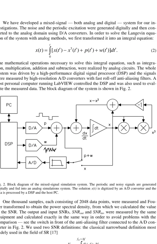
We have developed a mixed-signal — both analog and digital — system for our in-vestigations. The noise and the periodic excitation were generated digitally and then con-verted to the analog domain using D/A converters. In order to solve the Langevin equa-tion of the system with analog methods, we first transformed it into an integral equaequa-tion:





















t

d

t

w

t

p

t

x

t

x

t

x

.

)]

(

)

(

)

(

)

(

[

)

(

The mathematical operations necessary to solve this integral equation, such as integra-tion, multiplicaintegra-tion, addition and subtracintegra-tion, were realized by analog circuits. The whole system was driven by a high-performance digital signal processor (DSP) and the signals were measured by high-resolution A/D converters with fast roll-off anti-aliasing filters. A host personal computer running LabVIEW controlled the DSP and was also used to eval-uate the measured data. The block diagram of the system is shown in Fig. 2.

Fig. 2. Block diagram of the mixed-signal simulation system. The periodic and noisy signals are generated digitally and fed into an analog simulations system. The solution x(t) is digitized by an A/D converter and the data is processed by a DSP and the host PC.

One thousand samples, each consisting of 2048 data points, were measured and Fou-rier transformed to obtain the power spectral density, from which we calculated the value of the SNR. The output and input SNRs, SNRout and SNRin, were measured by the same equipment and calculated exactly in the same way in order to avoid problems with the comparison — see the switch in front of the anti-aliasing filter connected to the A/D con-verter in Fig. 2. We used two SNR definitions: the classical narrowband definition most widely used in the field of SR [17]

)

(

)

(

lim

f

S

df

f

S

SNR





and a wideband SNR given by the ratio of the total power of the deterministic part of the signal PS to the total power of the noise part PN:

.

)

(

)

(

lim











df

f

S

df

f

S

P

P

SNR

In the definitions above, f0 denotes the frequency of the deterministic signal, S(f) stands for the power spectral density of the signal and SN(f) signifies the power spectral density of the noise component in the signal. Note here that the classical narrowband definition has long been perceived as insufficient to describe noisy signals correctly. Researchers have introduced several alternative methods for characterizing the quality of signal trans-fer, such as those based on entropy [14, 18] or channel capacity [19]. The wideband defi-nition we suggest, SNRw, is usually applied in practical measurements and it reflects the quality of the transfer better than the narrowband SNR. Figure 3 highlights this fact, where SNR and SNRw is compared on a simple signal consisting of a sinusoidal plus noise. The 1V amplitude sinusoidal with frequency of 30 Hz was added to a 16 kHz bandwidth Gaussian white noise and this signal was filtered by a second order Butter-worth bandpass filter with cutoff frequencies of 20Hz and 40Hz. As one can expect, the noisy signal becomes much clearer after filtering, which is reflected only by SNRw, SNR is the same for both signals within the measurement error: SNR uses only a very small frequency range from the background noise around the signal frequency and the intensity of the noise in this range is altered by the same factor as that of the sinusoidal signal.

The SNR gain we are interested in is simply the ratio of the output SNR to the input SNR: in out

SNR

SNR

G



Of course, we also calculated a wideband gain from the wideband counterparts of SNRin and SNRout: w in w out w

SNR

SNR

G



0.0 0.1 0.2 0.3 0.4 0.5 -4 -3 -2 -1 0 1 2 3 4 Am pl itud e [ V] time [s] 0.0 0.1 0.2 0.3 0.4 0.5 -4 -3 -2 -1 0 1 2 3 4 Am pl itud e [ V] time [s] 0 20 40 60 80 100 1E-6 1E-5 1E-4 1E-3 0.01 0.1 SNR=4410 SNR_w=0.503 PS D [V 2 /Hz] Frequency [Hz] 0 20 40 60 80 100 1E-6 1E-5 1E-4 1E-3 0.01 0.1 SNR=4560 SNR_w=407 P S D [ V 2/Hz] Frequency [Hz]

Fig. 3. The plots on the left show 1V amplitude 30Hz frequency sinusoidal plus 16 kHz bandwidth Gaussian white noise and its power spectral density (PSD). Filtering this signal using a second order Butterworth bandpass filter with cutoff frequencies of 20 Hz and 40 Hz results in the signal presented on the right panel. It is easy to see that while the classical SNR is the same within the measurement error, SNRw and the time domain

signal reflect the improvement. SNR has a value of 4410 and 4560 while SNRw is obtained as 0.503 and 407 for

the original and filtered signal, respectively.

3. Results

We carried out our simulations and calculated the input and output SNRs as well as SNR gains for three different values of the amplitude of the deterministic signal (70%, 80% and 90% of threshold value) with duty cycles of 10%, 20% and 30% for each amplitude value. A sample length of 2048 was used for recordings and 1000 samples were averaged to compute the power spectral density and the SNR. The sampling frequency was 8 kHz, the frequency of the periodic input signal was set to 31.25 Hz and the bandwidth of the white noise was 50 kHz. We applied both the narrowband and wideband definition of the SNR; the independent variable in each case was the input noise amplitude. Apart from the basic question whether we can obtain SNR gains higher than unity, we examined how the values of the amplitude and duty cycle of the periodic signal influence the SNR and the SNR gain.

0.2 0.4 0.6 0.8 100 1000 10000 Signal amplitude OUT, 70% OUT, 80% OUT, 90% IN, 70% IN, 80% IN, 90% SNR  0.2 0.4 0.6 0.8 0.1 1 10 Signal amplitude 70% 80% 90% G 

Fig. 4. Input and output SNR and gain as functions of the input noise amplitude. The amplitude of the signal is 70%, 80% and 90% of the threshold value; the duty cycle is 10%. The amplitude of the noise is denoted by σ; its value is expressed in units normalized by the threshold.

0.2 0.4 0.6 0.8 0.1 1 10 100 Signal amplitude OUT, 70% OUT, 80% OUT, 90% IN, 70% IN, 80% IN, 90% S NR w  0.2 0.4 0.6 0.8 0.1 1 10 Signal amplitude 70% 80% 90% Gw 

Fig. 5.Wideband input and output SNR and gain as functions of the input noise amplitude. The amplitude of the signal is 70%, 80% and 90% of the threshold value; the duty cycle is 10%. The amplitude of the noise is denot-ed by σ; its value is expressed in units normalized by the threshold.

Figure 4 shows how the narrowband SNRin, SNRout and G depend on the input noise intensity for three different amplitudes of the periodic signal. We can conclude two things from this figure. First, SNR improvement is possible in the double-well potential — SNRout can be greater than SNRin over a certain range of input noise intensity. Second, the value of SNR gain is strongly influenced by the amplitude of the periodic signal, more precisely, higher gains are obtained for larger amplitudes. G exceeds unity only when the amplitude is 80% or greater, in other words, only in the strongly NLR limit.

Figure 5 is parallel to Fig. 4, only here the wideband quantities are plotted. Compar-ing these figures to each other, we see how much the SNR definition we use affects the results we get: with the wideband SNR, SNR improvement occurs for all three signal amplitudes and over a wider range of noise intensity than with the narrowband SNR. Fig-ure 6 shows the two types of gains side by side to illustrate the differences between them.

0.2 0.3 0.4 0.5 0.6 0.7 0.8 0.9 0.1 1 10 G G_w

G

Fig. 6.Narrowband (G) and wideband (Gw) SNR gains compared. The amplitude of the noise is denoted by σ;

its value is expressed in units normalized by the threshold.

In Fig. 7, we can observe how the value of the duty cycle affects the SNR gain, both narrowband and wideband.

0.2 0.3 0.4 0.5 0.6 0.7 0.8 0.1 1 10 Duty cycle 10% 20% 30% G  0.2 0.3 0.4 0.5 0.6 0.7 0.8 0.1 1 10 Duty cycle 10% 20% 30% Gw 

Fig. 7. The plot on the left shows SNR gain versus noise amplitude for different duty cycles of 10%, 20% and 30%. The right panel shows the same with wideband gain. The signal amplitude is 90% of the threshold value for all curves. The amplitude of the noise is denoted by σ; its value is expressed in units normalized by the threshold.

It is clear that increasing the duty cycle lowers the SNR gain. One can easily under-stand this fact: the output signal is similar for different duty cycles, which is reflected in similar SNRout values, while SNRin increases with greater duty cycles.

4. Conclusion

Using mixed signal simulation techniques, we have shown that one of the most common dynamical SR systems, the double well potential, can provide high SNR amplification if the input excitation is a periodic pulse train plus Gaussian white noise. We have also demonstrated that high SNR gains can be observed for small duty cycles and a signal

amplitude close to the switching threshold. Note here that our result is not in contradic-tion with the theoretical result that output SNR cannot exceed input SNR if the system works in the linear response range, since we used large signal amplitude somewhat below the switching threshold, which means that our system worked in the non-linear limit.

We would also like to emphasize that the SNR gain is greater than unity even over a wider range if we apply a much more realistic wideband definition based on the total power of signal and noise.

Acknowledgements

We thank L. B. Kish for helpful discussions.

References

[1] L. B. Kiss, Possible breakthrough: significant improvement of signal to noise ratio by stochas-tic resonance, in Chaotic, Fractal, and Nonlinear Signal Processing, Proc. Am. Institute Phys., ed. R. Katz, Mystic, Connecticut, USA(1996) 382–396.

[2] K. Loerincz, Z. Gingl and L. B. Kiss, A stochastic resonator is able to greatly improve signal-to-noise ratio, Phys Lett A224 (1996) 63–67.

[3] F. Chapeau-Blondeau and X. Godivier, Theory of stochastic resonance in signal transmission by static non-linear systems, Phys Rev E55 (1997) 1478–1495.

[4] D. G. Luchinsky and P. V. E. McClintock, Irreversibility of classical fluctuations studied in analogue electrical circuits, Nature389 (1997) 463–466.

[5] S. M. Bezrukov and I. Vodyanoy, Stochastic resonance in non-dynamical systems without re-sponse thresholds,Nature385 (1997) 319–321.

[6] S. Kadar, J. Wang and K. Showalter, Noise-supported traveling waves in sub-excitable media, Nature391 (1998) 770–773.

[7] S. M. Bezrukov and I. Vodyanoy, Noise-induced enhancement of signal-transduction across voltage-dependent ion channels,Nature378 (1995) 362–364.

[8] K. Wiesenfeld and F. Moss, Stochastic resonance and the benefits of noise from ice ages to crayfish and squids,Nature373 (1995) 33–36.

[9] J. M. G. Vilar, G. Gomila and J. M. Rubi, Stochastic resonance in noisy nondynamical systems, Phys Rev Lett81 (1998) 14–17.

[10] M. E. Inchiosa, A. R. Bulsara, A. D. Hibbs and B. R. Whitecotton, Signal enhancement in a nonlinear transfer characteristic,Phys Rev Lett80 (1998) 1381–1392.

[11] J. J. Collins, C. C. Chow and T. T. Imhoff, Aperiodic stochastic resonance in excitable sys-tems,Phys Rev E52 (1995) 3321–3324.

[12] L. B. Kiss, Z. Gingl, Z. Marton, J. Kertesz, F. Moss, G. Schmera and A. R. Bulsara, 1/f noise in systems showing stochastic resonance,J Stat Phys70 (1993) 451–462.

[13] M. I. Dykman, D. G. Luchinsky, R. Mannella, P. V. E. McClintock, N. D. Stein and N. G. Stocks, Stochastic resonance in perspective,Il Nuovo Cimento D 17D (1995) 661–683. [14] M. DeWeese and W. Z. Bialek, Information flow in sensory neurons,Il Nuovo Cimento D17D

(1995) 733–741.

[15] Z. Gingl, R. Vajtai and L. B. Kiss, Signal-to-noise ratio gain by stochastic resonance in a bistable system,Chaos, Solitons and Fractals11 (2000) 1929–1932.

[16] P. Hänggi, M. E. Inchiosa, D. Fogliatti and A. R. Bulsara, Nonlinear stochastic resonance: The saga of anomalous output-input gain,Phys Rev E62 (2000) 6155–6163.

[17] L. Gammaitoni, P. Hänggi, P. Jung and F. Marchesoni, Stochastic Resonance, Rev Mod Phys 70 (1998) 223–287.

[18] I. Goychuk and P. Hänggi, Stochastic resonance in ion channels characterized by information theory, Phys Rev E 61 (2000) 4272–4280.

[19] L. B. Kish, G. P. Harmer and D. Abbott, Information transfer rate of neurons: stochastic reso-nance of Shannon’s information channel capacity, Fluctuation and Noise Letters 1 (2001) L13–L19.