Expert Systems with Applications

Gradient boosting trees for auto insurance loss cost modeling and prediction

Leo Guelman

⇑

Royal Bank of Canada, RBC Insurance, 6880 Financial Drive, Mississauga, Ontario, Canada L5N 7Y5

a r t i c l e

i n f o

Keywords: Statistical learning Gradient boosting trees Insurance pricing

a b s t r a c t

Gradient Boosting (GB) is an iterative algorithm that combines simple parameterized functions with ‘‘poor’’ performance (high prediction error) to produce a highly accurate prediction rule. In contrast to other statistical learning methods usually providing comparable accuracy (e.g., neural networks and sup-port vector machines), GB gives interpretable results, while requiring little data preprocessing and tuning of the parameters. The method is highly robust to less than clean data and can be applied to classification or regression problems from a variety of response distributions (Gaussian, Bernoulli, Poisson, and Laplace). Complex interactions are modeled simply, missing values in the predictors are managed almost without loss of information, and feature selection is performed as an integral part of the procedure. These properties make GB a good candidate for insurance loss cost modeling. However, to the best of our knowl-edge, the application of this method to insurance pricing has not been fully documented to date. This paper presents the theory of GB and its application to the problem of predicting auto ‘‘at-fault’’ accident loss cost using data from a major Canadian insurer. The predictive accuracy of the model is compared against the conventional Generalized Linear Model (GLM) approach.

2011 Elsevier Ltd. All rights reserved.

1. Introduction

Generalized Linear Models (GLMs) (McCullagh & Nelder, 1989) are widely recognized as an accepted framework for building insurance pricing models. These models are based on a traditional approach to statistical modeling which starts by assuming that data are generated by a given stochastic data model (e.g., Gaussian, Gamma, Poisson, etc.). There is vast insurance pricing literature on such models (Anderson, Feldblum, Modlin, Schirmacher, & Thandi, 2007; Brockman & Wright, 1992; Haberman & Renshaw, 1996). They are attractive in the sense of producing interpretable param-eters which are combined in a multiplicative fashion to obtain an estimate ofloss cost, defined here as the portion of the premium which covers losses and related expenses (not including loadings for the insurance company’s expenses, premium taxes, contingen-cies, and profit margins). Model validation is usually done using goodness-of-fit tests and residual examination.

In the past two decades, the rapid development in computation and information technology has created an immense amount of data. The field of statistics was revolutionized by the creation of new tools that helped analyze the increasing size and complexity in the data structures. Most of these tools originated from an algo-rithmic modeling culture as opposed to a data modeling culture (Brieman, 2001). In contrast to data modeling, algorithmic model-ing does not assume any specific model for the data, but treats the

data mechanism as unknown. As a result, algorithmic models sig-nificantly increase the class of functions that can be approximated relative to data models. They are more efficient in handling large and complex data sets and in fitting non-linearities to the data. Model validation is measured by the degree of predictive accuracy and this objective is usually emphasized over producing interpret-able models. It is probably due to this lack of interpretability in most algorithmic models, that their application to insurance pric-ing problems has been very limited so far.Chapadoset al. (2001) used several data-mining methods to estimate car insurance pre-miums. Francis (2001)illustrates the application of neural net-works to insurance pricing problems such as the prediction of frequencies and severities.Kolyshkina, Wong, and Lim (2004) dem-onstrate the use of multivariate adaptive regression splines (MARS) to enhance GLM building. To the best of our knowledge, the appli-cation of Gradient Boosting (GB) to insurance pricing has not been fully documented to date.

Among algorithmic models, GB is unique in the sense of achiev-ing both predictive accuracy and model interpretation goals. The later objective is particularly important in business environments, where models must generally be approved by non-statistically trained decision makers who need to understand how the output from the ‘‘black-box’’ is being produced. In addition, this method requires little data preprocessing and tuning of the parameters. It is highly robust to less than clean data and can be applied to clas-sification or regression problems from a variety of response distri-butions. Complex interactions are modeled simply, missing values in the predictors are managed almost without loss of information, 0957-4174/$ - see front matter2011 Elsevier Ltd. All rights reserved.

doi:10.1016/j.eswa.2011.09.058

⇑ Tel.: +1 905 606 1175; fax: +1 905 286 4756. E-mail address:[email protected]

Contents lists available atSciVerse ScienceDirect

Expert Systems with Applications

j o u r n a l h o m e p a g e : w w w . e l s e v i e r . c o m / l o c a t e / e s w a

and feature selection is performed as an integral part of the proce-dure. These properties make this method a good candidate for insurance loss cost modeling.

The objective of this paper is to present the theory of GB and its application to the analysis of auto insurance loss cost modeling using data from a major Canadian insurer. We first define the scope of the predictive learning problem and the boosting approach to solve it. The core of the paper follows, comprising a detailed description of gradient boosting trees from the statistical learning perspective. We next describe an application to the analysis of auto insurance ‘‘at-fault’’ accident loss cost. A discussion is outlined at the end.

2. Predictive learning and boosting

The predictive learning problem can be characterized by a vec-tor of inputs or predicvec-tor variablesx= {x1,. . .,xp} and an output or target variabley. In this application, the input variables are repre-sented by a collection of quantitative and qualitative attributes of the vehicle and the insured, and the output is the actual loss cost. Given a collection ofMinstances {(yi,xi);i= 1,. . .,M} of known (y,x) values, the goal is to use this data to obtain and estimate of the function that maps the input vectorxinto the values of the outputy. This function can then be used to make predictions on instances where only thexvalues are observed. Formally, we wish to learn a prediction function ^fðxÞ:x!y that minimizes the expectation of some loss functionL(y,f) over the joint distribution of all (y,x)-values

^

fðxÞ ¼argminfðxÞEy;xLðy;fðxÞÞ ð1Þ

Boosting methods are based on the intuitive idea that combin-ing many ‘‘weak’’ rules to approximate (1) should result in classification and regression models with improved predictive per-formance compared to a single model. A weak rule is a learning algorithm which performs only a little bit better than a coinflip. The aim is to characterize ‘‘local rules’’ relating variables (e.g., ‘‘if an insured characteristic A is present and B is absent, then a claim has high probability of occurring’’). Although this rule alone would not be strong enough to make accurate predictions on all insureds, it is possible to combine many of those rules to produce a highly accurate model. This idea, known as the ‘‘the strength of weak lear-nability’’ (Schapire, 1990) was originated in the machine learning community with the introduction ofAdaBoost, which is described in the next section.

3. AdaBoost

The AdaBoost is a popular boosting algorithm due toFreund and Schapire (1996). Consider a classification problem with a binary response variable coded as y2{1, 1} and classifier ^fðxÞ taking one of those two values {1, 1}. The AdaBoost algorithm is outlined below. In short, the algorithm generates a sequence of weak classi-fiers induced on a distribution of weights over the training set. One such weak classifier often used in AdaBoost is a single-split classi-fication tree with only two terminal nodes. Initially, all observation weights are set equally, but on each iteration, the training observa-tions that were misclassified in the previous step receive more weight in the next iteration. Thus, the algorithm is forced to focus on observations that are difficult to correctly classify with each successive iteration. The final classifier is a weighted majority vote of the individual weak classifiers. The weight assigned to each weak classifier gets larger as its weighted error rate measured on the training set gets smaller.

Algorithm 1.AdaBoost

1: Initialize observation weightswi¼M1 2:fort= 1 toTdo

3: Fitft(x) as the weak classifier on the training data usingwi 4: Compute the weighted error rate aserrt¼

Pm

i¼1wiIðyi–ftðxiÞÞ

Pm i¼1wi 5: Let

a

t= log ((1errt)/errt)

6: Updatewi wi.exp[

a

t.I(yi–ft(xi))] scaled to sum to one" i2{1,. . .,M}

7:end for

8: Output^fðxÞ ¼sign PTt¼1

a

t:^ftðxÞ

h i

The success of AdaBoost for classification problems was seen as a mysterious phenomenon by the statistics community until (Friedman, Hastie, & Tibshirani, 2000) showed the connection between boosting and statistical concepts such as additive model-ing and maximum-likelihood. Their main result is that it is possi-ble to rederive AdaBoost as a method for fitting an additive model in a forward stagewise manner. This gave significant understand-ing of why this algorithm tends to outperform a sunderstand-ingle base mod-el: by fitting an additive model of different and potentially simple functions, it expands the class of functions that can be approximated.

4. Additive models and boosting

Our discussion in this section will be focused on the regres-sion problem, where the outputyis quantitative and the objec-tive is to estimate the mean E(yjx) =f(x). The standard linear regression model assumes a linear form for this conditional expectation

EðyjxÞ ¼fðxÞ ¼X p

j¼1

bjxj ð2Þ

An additive model extends the linear model by replacing the linear component

g

¼Ppj¼1bjxj with an additive predictor of the form

g

¼Pp_j¼1fjðxjÞ. We assume

EðyjxÞ ¼fðxÞ ¼X p

j¼1

fjðxjÞ; ð3Þ

where f1(),. . .,fp() are smooth functions. There is a separate smooth functionfjfor each of thepinput variablesxjor, more gen-erally, each componentfjis a function of a prespecified subset of the input variables. These functions are not assumed to have a paramet-ric form, but instead they are estimated in a non-parametparamet-ric fashion.

This model can be extended by considering additive models with functionsft(x),t= {1,. . .,T} of potentially all the inputs vari-ables. In this context

fðxÞ ¼X T t¼1 ftðxÞ ¼X T t¼1 bthðx;atÞ; ð4Þ

where the functionsh(x;at) are usually taken to be simple functions characterized by a set of parametersa= {a1,a2,. . .} and a multiplierbt. This form includes models such as neural networks, wavelets, multi-variate adaptive regression splines and regression trees (Hastie, Tibshirani, & Friedman, 2001). In a boosting context, bth(x;at)

represents the ‘‘weak learner’’ andf(x) the weighted majority vote of the individual weak learners.

Estimation of the parameters in(4)amounts to solving

min fbt;atgT1 XM i¼1 L yi; XT t¼1 bthðxi;atÞ ! ; ð5Þ

whereL(y,f(x)) is the chosen loss function(1)to define lack-of-fit. A ‘‘greedy’’ forward stepwise method solves(5)by sequentially fitting a single weak learner and adding it to the expansion of prior fitted terms. The corresponding solution values of each new fitted term is not readjusted as new terms are added into the model. This is out-lined in Algorithm 2.

Algorithm 2.Forward Stagewise Additive Modeling

1: Initializef0(x) = 0 2:fort= 1 toTdo

3: Obtain estimatesbtandatby minimizing

PM

i¼1Lðyi;ft1ðxiÞ þbhðxi;aÞÞ 4: Updateft(x) =ft1(x) +bth(x;at)

5:end for

6: Output^fðxÞ ¼fTðxÞ

If squared-error is used as the loss function, line 3 simplifies to Lðyi;ft1ðxiÞ þbhðxi;aÞÞ ¼ ðyift1ðxiÞ bhðxi;aÞÞ2

¼ ðritbhðxi;aÞÞ2; ð6Þ where rit is the residual of the ith observation at the current iteration. Thus, for squared-error loss, the termbth(x;at) fitted to the current residuals is added to the expansion in line 4. It is also fairly easy to show (Hastie et al., 2001) that the AdaBoost algorithm described in Section3is equivalent to forward stagewise modeling based on an exponential loss function of the form L(y,f(x)) =exp(yf(x)).

5. Gradient boosting trees

Squared-error and exponential error are plausible loss functions commonly used for regression and classification problems, respec-tively. However, there may be situations in which other loss func-tions are more appropriate. For instance, binomial deviance is far more robust than exponential loss in noisy settings where the Bayes error rate is not close to zero, or in situations where the tar-get classes are mislabeled. Similarly, the performance of squared-error significantly degrades for long-tailed squared-error distributions or the presence of ‘‘outliers’’ in the data. In such situations, other functions such as absolute error or Huber loss are more appropriate.

Under these alternative specifications for the loss function and for a particular weak learner, the solution to line 3 in Algorithm 2 is difficult to obtain. The gradient boosting algorithm solves the problem using a two-step procedure which can be applied to any differentiable loss function. The first step estimatesatby fitting a weak learnerh(x;a) to the negative gradient of the loss function (i.e., the ‘‘pseudo-residuals’’) using least-squares. In the second step, the optimal value ofbtis determined givenh(x;at). The pro-cedure is shown in Algorithm 3.

Algorithm 3.Gradient Boosting

1: Initializef0(x) to be a constant,f0ðxÞ ¼argminb PM

i¼1Lðyi;bÞ 2:fort= 1 toTdo

3: Compute the negative gradient as the working response ri¼ @Lðyi;fðxiÞÞ @fðxiÞ fðxÞ¼ft1ðxÞ ;i¼ f1;. . .;Mg

4: Fit a regression model toriby least-squares using the inputxiand get the estimateatofbh(x;a)

5: Get the estimatebtby minimizing L(yi,ft1(xi) +bh(xi;at))

6: Updateft(x) =ft1(x) +bth(x;at)

7:end for

8: Output^fðxÞ ¼fTðxÞ

For squared-error loss, the negative gradient in line 3 is just the usual residuals, so in this case the algorithm is reduced to standard least-squares boosting. With absolute error loss, the negative gra-dient is the sign of the residuals. Least-squares is used in line 4 independently of the chosen loss function.

Although boosting is not restricted to trees, our work will focus on the case in which the weak learners represent a ‘‘small’’ regres-sion tree, since they were proven to be a convenient representation for the weak learnersh(x;a) in the context of boosting. In this spe-cific case, the algorithm above is calledgradient boosting treesand the parametersatrepresent the split variables, their split values and the fitted values at each terminal node of the tree. Henceforth in this paper, the term ‘‘Gradient Boosting’’ will be used to denote gradient boosting trees.

6. Injecting randomness and regularization

Two additional ingredients to the gradient boosting algorithm were proposed by Friedman, namely regularization through shrinkage of the contributed weak learners (Friedman, 2001) and injecting randomness in the fitting process (Friedman, 2002).

The generalization performance of a statistical learning method is related to its prediction capabilities on independent test data. Fitting a model too closely to the train data can lead to poor gen-eralization performance. Regularization methods are designed to prevent ‘‘overfitting’’ by placing restrictions on the parameters of the model. In the context of boosting, this translates into control-ling the number of iterationsT(i.e., trees) during the training pro-cess. An independent test sample or cross-validation can be used to select the optimal value of T. However, an alternative strategy showed to provide better results, and relates to scaling the contri-bution of each tree by a factor

s

2(0, 1]. This implies changing line 6 in Algorithm 3 to

ftðxÞ ¼ft1ðxÞ þ

s

bthðx;atÞ ð7Þ The parameter

s

has the effect of retarding the learning rate of the series, so the series has to be longer to compensate for the shrinkage, but its accuracy is better. Lower values of

s

will produce a larger value forTfor the same test error. Empirically it has been shown that small shrinkage factors (

s

< 0.1) yield dramatic improvements over boosting series built with no shrinkage (

s

= 1). The trade-off is that a small shrinkage factor requires a higher number of iterations and computational time increases. A

strategy for model selection often used is practice is to set the value of

s

as small as possible (i.e. between 0.01 and 0.001) and then chooseTby early stopping.

The second modification introduced in the algorithm was to incorporate randomness as an integral part of the fitting procedure. This involves taking a simple random sample without replacement of usually approximately 1/2 the size of the full training data set at each iteration. This sample is then used to fit the weak learner (line 4 in Algorithm 3) and compute the model update for the current iteration. As a result of this randomization procedure, the variance of the individual weak learner estimates at each iteration increases, but there is less correlation between these estimates at different iterations. The net effect is a reduction in the variance of the combined model. In addition, this randomization procedure has the benefit of reducing the computational demand. For instance, taking half-samples reduces computation by almost 50%. 7. Interpretation

Accuracy and interpretability are two fundamental objectives of predictive learning. However, these objectives do not always coin-cide. In contrast to other statistical learning methods providing comparable accuracy (e.g., neural networks and support vector machines), gradient boosting gives interpretable results. An impor-tant measure often useful for interpretation is the relative influ-ence of the input variables on the output. For a single decision tree, (Brieman, Friedman, Olshen, & Stone, 1984) proposed the following measure as an approximation of the relative influence of a predictorxj bI2 j ¼ X all splits onxj ^

m

2 s; ð8Þ where^

m

2

s is the empirical improvement in squared-error as a result of usingxjas a splitting variable at the non-terminal nodes. For Gra-dient Boosting, this relative influence measure is naturally extended by averaging(8)over the collection of trees.

Another important interpretation component is given by a visual representation of the partial dependence of the approxima-tion^fðxÞon a subsetx‘of size‘<pof the input vectorx. The

depen-dency of^fðxÞon the remaining predictorsxc(i.e.x‘[xc=x) must be conditioned out. This can be estimated based on the training data by ^ fðx‘Þ ¼ 1 M XM i¼1 ^_fðx ‘;xicÞ ð9Þ

Note that this method requires predicting the response over the training sample for each set of the joint values ofx‘, which can be

computationally very demanding. However, for regression trees, a weighted transversal method (Friedman, 2001) can be used, from which^fðx‘Þis computed using only the tree, without reference to

the data itself.

8. Application to auto insurance loss cost modeling 8.1. The data

The data used for this analysis were extracted from a large data-base from a major Canadian insurer. It consists of policy and claim information at the individual vehicle level. There is one observa-tion for each period of time during which the vehicle was exposed to the risk of having an at-fault collision accident. Mid-term changes and policy cancellations would result in a corresponding reduction in the exposure period.

The data set includes 426,838 earned exposures (measured in vehicle-years) from Jan-06 to Jun-09, and 14,984 claims incurred during the same period of time, with losses based on best reserve estimates as of Dec-09. The input variables (for an overview, see Table 1) were measured at the start of the exposure period, and are represented by a collection of quantitative and qualitative attri-butes of the vehicle and the insured. The output is the actualloss cost, which is calculated as the ratio of the total amount of losses to the earned exposure. In practice, the insurance legislation may restrict the usage of certain input variables to calculate insurance premiums. Although our analysis was developed assuming a free rating regulatory environment, the techniques described here can be applied independently of the limitations imposed by any spe-cific legislation.

For statistical modeling purposes, we first partitioned the data into train (70%) and test (30%) data sets. The train set was used for model training and selection, and the test set to assess the pre-dictive accuracy of the selected gradient boosting model against the Generalized Linear Model. To ensure that the estimated perfor-mance of the model, as measured on the test sample, is an accurate approximation of the expected performance on future ‘‘unseen’’ cases, the inception date of policies in the test set is posterior to the one of policies used to build and select the model.

Loss cost is usually broken down into two components:claim frequency(calculated as the ratio of the number of claims to the earned exposure) andclaim severity(calculated as the ratio of the total amount of losses to the number of claims). Some factors affect claim frequency and claim severity differently, and thus we consid-ered them separately. For the claim frequency model, the target variable was coded as binary since only a few records had more than one claim during a given exposure period. The exposure per-iod was treated as anoffsetvariable in the model (i.e., a variable with a known parameter of 1).

The actual claim frequency measured on the entire sample is 3.51%. This represents an imbalanced or skewed class distribution for the target variable, with one class represented by a large sam-ple (i.e. the non-claimants) and the other represented by only a few (i.e. the claimants). Classification of data with imbalanced class distribution has posed a significant drawback for the performance attainable by most standard classifier algorithms, which assume a relatively balanced class distribution (Sun, Kamel, Wong, & Wang, 2007). These classifiers tend to output the simplest hypothesis which best fits the data and, as a result, classification rules that predict the small class tend to be fewer and weaker compared to those that predict the majority class. This may hinder the detection of claim predictors and eventually decrease the predictive accuracy of the model. To address this issue, we re-balanced the class distri-bution for the target in the frequency model by resampling the data space. Specifically, we under-sampled instances from the majority class to attain a 10% representation of claims in the train sample. The test sample was not modified and thus contains the original class distribution for the target. In econometrics, this sam-ple scheme is known aschoice-basedor endogenous stratified sam-pling (Green, 2000) and it is also popular in the computer science community (Chan & Stolfo, 1998; Estabrooks & Japkowicz, 2004). The ‘‘optimal’’ class distribution for the target variable based on under-sampling is generally dependent on the specific data set (Weiss & Provost, 2003), and it is usually considered as an addi-tional tuning parameter to optimize based on the performance measured on a validation sample.

The estimation of a classification model from a balanced sample can be efficient but will overestimate the actual claim frequency. An appropriate statistical method is required to correct this bias, and several alternatives exist for that purpose. In this application, we used the method of prior correction, which fundamentally involves adjusting the predicted values based on the actual claim

frequency in the population. This correction is described for the logit model in Ref. (King & Zeng, 2001), and the same method has been successfully used in a boosting application to predict cus-tomer churn (Lemmens & Croux, 2006).

8.2. Building the model

The first choice in building the model involves selecting an appropriate loss function L(y,f(x)) as in (1). Squared-error loss,

PM

i¼1ðyifðxiÞÞ2, and Bernoulli deviance, 2PMi¼1ðyifðxiÞ logð1þ expðfðxiÞÞÞ, were used to define prediction error for the severity and frequency models, respectively. Then, it is necessary to select the shrinkage parameter

s

applied to each tree and the sub-sam-pling rate as defined in Section6. The former was set at the fixed value of 0.001 and the later at 50%. Next, the the size of the individ-ual treesSand the number of boosting iterationsT(i.e., number of trees) need to be selected. The size of the trees was selected by sequentially increasing the interaction depth of the tree, starting with an additive model (single-split regression trees), followed by two-way interactions, and up to six-way interactions. This

was done in turn for the frequency and severity models. For each of these models, we run 20,000 boosting iterations using the train-ing data set.

A drawback of the under-sampling scheme described in Section 8.1, is that we may risk losing information from the majority class when being under-sampled. To maximize the usage of the informa-tion available in the training data, the optimal value for the param-eters S and T was chosen based on the smallest estimated prediction error using a K-fold cross-validation procedure with K= 10. This involves splitting the training data inKequal parts, fit-ting the model toK1 parts of the data, and then calculating the value for the prediction error on the kth part. This is done for k= 1, 2,. . .,Kand then the Kestimated values for the prediction error are averaged. Using a three-way interaction gave best results in both frequency and severity models. Based on this level of inter-action,Fig. 1shows the train and cv-error as function of the num-ber of iterations for the severity model. The optimal value ofTwas set at the point for which the cv-error cease to decrease.

The test data set was not used for model selection purposes, but to assess the generalization error of the final chosen model relative to the Generalized Linear Model approach. The later model was estimated based on the same training data and using Binomial/ Gamma distributions for the response variables in the Frequency/ Severity models, respectively.

8.3. Results

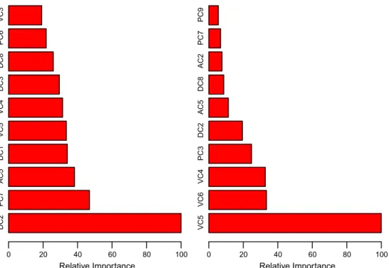
Fig. 2displays the relative importance of the 10 most influential predictor variables for the frequency (left) and severity (right) mod-els. Since these measures are relative, a value of 100 was assigned to the most important predictor and the others were scaled accord-ingly. There is a clear differential effect between the models. For instance, the number ofyears licensedof the principal operator of the vehicle is the most relevant predictor in the frequency model, while it is far less important in the severity model. Among the other influential predictors in the frequency model, we find the presence of an occasional driver under 25 years, thenumber of driving convictions, and theageof the principal operator. For the severity model, thevehicle ageis the most influential predictor, followed by theprice of the vehicleand thehorse power to weight ratio. Partial dependence plots offer additional insights in the way these vari-ables affect the dependent variable in each model. Fig. 3shows the partial dependence plots for the frequency model. The vertical scale is in the log odds and the hash marks at the base of each plot show the deciles of the distribution of the corresponding variable.

Table 1

Overview of loss cost predictors.

Driver characteristics Accident/conviction history Policy characteristics Vehicle characteristics DC1. Age of principal

operator

AC1. Number of chargeable accidents (last 1–3 years) PC1. Years since policy inception VC1. Vehicle make

DC2. Years licensed AC2. Number of chargeable accidents (last 4–6 years) PC2. Presence of multi-vehicle VC2. Vehicle purchased new or used

DC3. Age licensed AC3. Number of non-chargeable accidents (last 1–3 years)

PC3. Collision deductible VC3. Vehicle leased DC4. License class AC4. Number of non-chargeable accidents (last 4–6

years)

PC4. Billing type VC4. Horse power to weight ratio DC5. Gender AC5. Number of driving convictions (last 1–3 years) PC5. Billing status VC5. Vehicle age

DC6. Marital status AC6. Prior examination costs from accident-benefit claims

PC6. Rating territory VC6. Vehicle price DC7. Prior facility

association

PC7. Presence of occasional driver under 25

DC8. Postal code risk score PC8. Presence of occasional driver over

25

DC9. Insurance lapses PC9. Group business

DC10. Insurance suspensions

PC10. Business origin PC11. Dwelling unit type

0 5000 10000 15000 25000 26000 27000 28000 29000 Boosting Iterations Squared−Error Loss Train Error CV−Error

Fig. 1.The relation between train and cross validation error and the optimal number of boosting iterations (shown by the vertical green line). (For interpretation of the references to colour in this figure legend, the reader is referred to the web version of this article.)

The partial dependence of each predictor accounts for the average joint effect of the other predictors in the model.

Claim frequency has a nonmonotonic partial dependence on years licensed. It decreases over the main body of the data and

increases nearly at the end. The partial dependence onageinitially decreases abruptly up to a value of approximately 30, followed by a long plateau up to 70, when it steeply increases. The variables vehicle ageandpostal code risk scorehave a roughly monotonically

DC2 PC7 AC5 DC1 VC5 VC4 DC3 DC8 PC6 VC3 Relative Importance 0 20 40 60 80 100 VC5 VC6 VC4 PC3 DC2 AC5 DC8 AC2 PC7 PC9 Relative Importance 0 20 40 60 80 100

Fig. 2.Relative importance of the predictors for the Frequency (left) and Severity (right) models.

0 10 20 30 40 50 60 −2.4 −2.2 −2.0 −1.8 DC2 par tial dependence N Y −2.3 −2.2 −2.1 −2.0 −1.9 PC7 par tial dependence 0 1 2 −2.30 −2.20 −2.10 −2.00 AC5 par tial dependence 20 30 40 50 60 70 80 −2.3 −2.2 −2.1 −2.0 DC1 par tial dependence 0 5 10 15 −2.6 −2.5 −2.4 −2.3 −2.2 VC5 par tial dependence 550 600 650 700 750 800 850 −2.30 − 2.25 −2.20 − 2.15 −2.10 DC8 par tial dependence

decreasing partial dependence. The age of the vehicle is widely recognized as an important predictor in the frequency model (Brockman & Wright, 1992), since it is believed to be negatively associated with annual mileage. It is not a common practice to use annual mileage directly as an input in the model, due to the difficulty in obtaining a reliable estimate for this variable. Claim frequency is also estimated to increase with the number of driving convictions and it is higher for vehicles with an occasional driver under 25 years of age.

Note that these plots are not necessarily smooth, since there is no smoothness constraint imposed on the fitting procedure. This is the consequence of using a tree-based model. If a smooth trend is observed, this is result of the estimated nature of the depen-dence of the predictors on the response and it is purely dictated by the data.

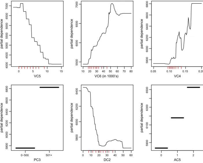
Fig. 4shows the partial dependence plots for the severity mod-el. The nature of the dependence ofvehicle ageandprice of the vehi-cleis naturally due to the fact that newer and more expensive cars would cost more to repair in the event of a collision. The shape of these curves is fairly linear over the vast majority of the data. The variable horse power to weight ratiomeasures the actual perfor-mance of the vehicle’s engine. The upward trend observed in the curve is anticipated, since drivers with high performance engines will generally drive at a higher speed compared to those with low performance engines. All the remaining variables have the expected partial dependence effect on claim severity.

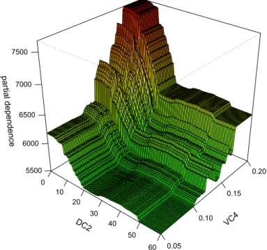
An interesting relationship is given inFig. 5, which shows the joint dependence betweenyears licensedandhorse power to weight

ratioon claim severity. There appears to be an interaction effect between these two variables. Claim severity tends to be higher for low values ofyears licensed, but this relation tends to be much stronger for high values ofhorse power to weight ratio.

We next compare the predictive accuracy of Gradient Boosting (GB) against the conventional Generalized Linear Model (GLM) approach based on the test sample. This was done by calculating the ratio of the rate we would charge based on the GB model to the rate we would charge based on the GLM. Then we grouped the observations into five fairly equally sized buckets ranked by the ratio. Finally, for each bucket we calculated the GLM-loss ratio, defined as the ratio of the actual losses to the GLM predicted loss cost. Fig. 6 displays the results. Note that the GLM-loss ratio increases whenever the GB model would suggest to charge a higher rate relative to the GLM. The upward trend in the GLM-loss ratio curve indicates the higher predictive performance of GB relative to GLM.

9. Discussion

In this paper, we described the theory of Gradient Boosting (GB) and its application to the analysis of auto insurance loss cost mod-eling. GB was presented as an additive model that sequentially fits a relatively simple function (weak learner) to the current residuals by least-squares. The most important practical steps in building a model using this methodology have been described. Estimating loss cost involves solving regression and classification problems

0 5 10 15 4000 4500 5000 5500 6000 6500 7000 VC5 partial dependence 10 20 30 40 50 60 70 80 5500 6000 6500 7000 VC6 (in 1000’s) partial dependence 0.05 0.10 0.15 0.20 5800 6000 6200 6400 6600 6800 VC4 partial dependence 0−500 501+ 5800 6000 6200 6400 6600 6800 PC3 partial dependence 0 10 20 30 40 50 60 5800 6000 6200 6400 DC2 partial dependence 0 1 2 5900 6100 6300 6500 AC5 partial dependence

with several challenges. The large number of categorical and numerical predictors, the presence of non-linearities in the data and the complex interactions among the inputs is often the norm. In addition, data might not be clean and/or contain missing values for some predictors. GB fits very well this data structure. First, based on the sample data used in this analysis, the level of accu-racy in prediction was shown to be higher for GB relative to the conventional Generalized Linear Model approach. This is not sur-prising since GLMs are, in essence, relatively simple linear models and thus they are constrained by the class of functions they can approximate. Second, as opposed to other non-linear statistical learning methods such as neural networks and support vector machines, GB provides interpretable results via the relative influ-ence of the input variables and their partial dependinflu-ence plots. This is a critical aspect to consider in a business environment, where models usually must be approved by non-statistically trained deci-sion makers who need to understand how the output from the ‘‘black-box’’ is being produced. Third, GB requires very little data preprocessing which is one of the most time consuming activities in a data mining project. Lastly, model selection is done as an

integral part of the GB procedure, and so it requires little ‘‘detec-tive’’ work on the part of the analyst.

In short, Gradient Boosting is a good alternative method to Gen-eralized Linear Models for building insurance loss cost models. The free available packagegbmimplements gradient boosting methods under the R environment for statistical computing (Ridgeway, 2007).

Acknowledgments

I am deeply grateful to Matthew Buchalter and Charles Dugas for thoughtful discussions. Also special thanks to Greg Ridgeway for freely distributing the gbm software package in R. Comments are welcome.

References

Anderson, D., Feldblum, S., Modlin, C., Schirmacher, D. Schirmacher, E., & Thandi, N. (2007). A practitioner’s guide to generalized linear models. Casualty Actuarial Society (CAS), Syllabus Year: 2010, Exam Number: 9, 1–116.

DC2 0 10 20 30 40 50 60 VC4 0.05 0.10 0.15 0.20 par tial dependence 5500 6000 6500 7000 7500

Fig. 5.Partial dependence of claim severity onyears licensedandhorse power to weight ratio.

(0.418,0.896] (0.896,0.973] (0.973,1.05] (1.05,1.15] (1.15,3.36]

Ratio: GB Pred. Loss Cost / GLM Pred. Loss Cost

Exposure Count 0 5000 10000 15000 0.9 1.0 1.1 1.2 1.3

Actual Losses/GLM Pred. Loss Cost

Brieman, L., Friedman, J., Olshen, R., & Stone, C. (1984).Classification and regression trees. CRC Press.

Brieman, L. (2001). Statistical modeling: The two cultures.Statistical Science, 16, 199–231.

Brockman, M., & Wright, T. (1992). Statistical motor rating: Making effective use of your data.Journal of the Institute of Actuaries, 119, 457–543.

Chan, P., & Stolfo, S. (1998). Toward scalable learning with non-uniform class and cost distributions: A case study in credit card fraud detection.Proceedings of the International Conference on Knowledge Discovery and Data Mining, 4(pp. 164– 168).

Chapados, N., Bengio, Y., Vincent, P., Ghosn, J., Dugas, C., Takeuchi, I., et al. (2001). Estimating car insurance premia: A case study in high-dimensional data inference. University of Montreal, DIRO Technical Report, 1199.

Estabrooks, T., & Japkowicz, T. (2004). A multiple resampling method for learning from imbalanced data sets.Computational Intelligence, 20, 315–354.

Francis, L. (2001). Neural networks demystified.Casualty Actuarial Society Forum, Winter, 2001, 252–319.

Freund, Y., & Schapire, R. (1996). Experiments with a new boosting algorithm. Proceedings of the International Conference on Machine Learning, 13(pp. 148– 156).

Friedman, J., Hastie, T., & Tibshirani, R. (2000). Additive logistic regression: A statistical view of boosting.The Annals of Statistics, 28, 337–407.

Friedman, J. (2001). Greedy function approximation: A gradient boosting machine. The Annals of Statistics, 29, 1189–1232.

Friedman, J. (2002). Stochastic gradient boosting.Computational Statistics & Data Analysis, 38, 367–378.

Green, W. (2000).Econometric analysis(4th ed.). Prentice-Hall.

Haberman, S., & Renshaw, A. (1996). Generalized linear models and actuarial science.Journal of the Royal Statistical Society, Series D, 45, 407–436. Hastie, T., Tibshirani, R., & Friedman, J. (2001).The elements of statistical learning.

Springer.

King, G., & Zeng, L. (2001). Explaining rare events in international relations. International Organization, 55, 693–715.

Kolyshkina, I., Wong, S., & Lim, S. (2004). Enhancing generalised linear models with data mining. Casualty Actuarial Society 2004, Discussion Paper Program. Lemmens, A., & Croux, C. (2006). Bagging and boosting classification trees to predict

churn.Journal of Marketing Research, 43, 276–286.

McCullagh, P., & Nelder, J. (1989).Generalized linear models(2nd ed.). Chapman and Hall.

Ridgeway, G. (2007). Generalized boosted models: a guide to the gbm package. Available fromhttp://cran.r-project.org/web/packages/gbm/index.html. Schapire, R. (1990). The strength of weak learnability.Machine Learning, 5, 197–227. Sun, Y., Kamel, M., Wong, A., & Wang, Y. (2007). Cost-sensitive boosting for

classification of imbalanced data.Pattern Recognition, 40, 3358–3378. Weiss, G., & Provost, F. (2003). Learning when training data are costly: The effect of

class distribution on tree induction.Journal of Artificial Intelligence Research, 19, 315–354.