Currency Carry Trades

(1)

NBER WORKING PAPER SERIES

CURRENCY CARRY TRADES

Travis J. Berge

Òscar Jordà

Alan M. Taylor

Working Paper 16491

http://www.nber.org/papers/w16491

NATIONAL BUREAU OF ECONOMIC RESEARCH

1050 Massachusetts Avenue

Cambridge, MA 02138

October 2010

Paper presented at the NBER International Seminar on Macroeconomics, Amsterdam, June 2010.

Taylor has been supported by the Center for the Evolution of the Global Economy at UC Davis and

Jordà by DGCYT Grant (SEJ2007-63098-econ); part of this work was completed whilst Taylor was

a Houblon-Norman/George Fellow at the Bank of England; all of this research support is gratefully

acknowledged. We thank Craig Burnside for sharing his data on risk factors with us. We acknowledge

helpful comments from our discussants Robert Cumby and Mark Taylor, and from participants at the

ISOM meeting, and we thank De Nederlandsche Bank for their efficient organization and warm hospitality.

All errors are ours. The views expressed herein are those of the authors and do not necessarily reflect

the views of the National Bureau of Economic Research.

NBER working papers are circulated for discussion and comment purposes. They have not been

peer-reviewed or been subject to the review by the NBER Board of Directors that accompanies official

NBER publications.

text, not to exceed two paragraphs, may be quoted without explicit permission provided that full credit,

including © notice, is given to the source.

(2)

Currency Carry Trades

Travis J. Berge, Òscar Jordà, and Alan M. Taylor

NBER Working Paper No. 16491

October 2010

JEL No. C44,F31,F37,G14,G15,G17

ABSTRACT

A wave of recent research has studied the predictability of foreign currency returns. A wide variety

of forecasting structures have been proposed, including signals such as carry, value, momentum, and

the forward curve. Some of these have been explored individually, and others have been used in combination.

In this paper we use new econometric tools for binary classification problems to evaluate the merits

of a general model encompassing all these signals. We find very strong evidence of forecastability

using the full set of signals, both in sample and out-of-sample. This holds true for both an unweighted

directional forecast and one weighted by returns. Our preferred model generates economically meaningful

returns on a portfolio of nine major currencies versus the U.S. dollar, with favorable Sharpe and skewness

characteristics. We also find no relationship between our returns and a conventional set of so-called

risk factors.

Travis J. Berge

Department of Economics

University of California, Davis

One Shields Ave

Davis, CA 95616

tjberge@ucdavis.edu

Òscar Jordà

Department of Economics

University of California, Davis

One Shields Ave.

Davis, CA 95616

ojorda@ucdavis.edu

Alan M. Taylor

Morgan Stanley

1585 Broadway

New York, NY 10023

and NBER

alan.taylor@morganstanley.com

(3)

1

Introduction

One of the oldest and most frequently recurring questions in international finance concerns the efficiency of the foreign exchange market. Indeed it is one of the most durable and intriguing questions in the field of finance as a whole since the market for major currencies is one of the largest, most liquid, and most actively-traded asset markets in existence. Thus, treated as a laboratory, this market more than any other may have the potential to reveal how close actual financial markets are to attaining their textbook idealized form: are asset returns essentially random or do they have systematically predictable elements?1

For several decades a long literature has sought to explore whether currency returns are fore-castable, and the simple “carry trade” logic of trading based on the interest differential has been very widely studied. Here, systematic ex-post profits are widely observed, a phenomenon which is merely a manifestation of the long-studied forward discount puzzle (see, e.g., Frankel 1980; Fama 1984; Hodrick 1987; Froot and Thaler 1990; Bekaert and Hodrick 1993; Engel 1996). Notwith-standing this broadly accepted puzzle, a number of metrics have been used to evaluate the pre-dictability and profitability of exchange rate forecasts and the results have by no means created consensus. Researchers have asked whether such forecasting power delivers statistically significant fit relative to random walk, and if the forecast can generate economically significant profits for a risk-neutral investor after transaction costs (Meese and Rogoff 1983; Kilian and M. Taylor 2003). Researchers have also sought to account for the possibility of time varying risk premia—but must then navigate between the inevitably circular reasoning that ex-post risk premia could be found that in principle explain any ex-post returns observed, and the problem that observable so-called risk factors are (apart from consumption growth) often atheoretic and ad hoc regressors vulnerable to a “ketchup” critique.2

Carry trades are now under scrutiny again. In conjunction with a dramatic rise in real-world currency trading in the last decade, a recent wave of research on exchange rate forecastability has appeared in the last few years asking new questions and sharpening new tools. Much of this literature has continued to focus on strategies based on the na¨ıve carry signal, where investors go long high-yield currencies, and short low-yield currencies (e.g., Brunnermeier, Nagel, and Pedersen 2008; Burnside, Eichenbaum and Kleshchelski 2006, 2008ab). These pre-financial-crisis studies also often found attractive residual profits, with moderately impressive Sharpe ratios. However, the strategies often came with unattractive third moments, with high negative skew resulting from the occasional tendency of target currencies to crash, or conversely funding currencies to suddenly appreciate (e.g., the well-known Japanese yen events of 1998). Whilst one could in principle truncate the downside risks by augmenting the strategy with put options (Burnside et al. 2008b; Clarida, Davis and Pedersen, 2009; Jurek 2008), these insurance mechanisms are not inexpensive, and entail the further complication of making assumptions concerning liquidity and counterparty risk in derivative markets.

1_{For a full survey of foreign exchange market efficiency see Chapter 2 in Sarno and M. Taylor (2002).} 2_{The critique is due to Summers (1985), who downplayed the usefulness of approaches which show that the prices} of all risky assets move up and down in unison—like the prices of different sized bottles of tomato ketchup—without offering either theoretical insights or empirical evidence as to the fundamental shocks behind such comovements.

(4)

The working of the foreign exchange market during the financial crisis challenged some of these findings. Investors using pure carry strategies fared very poorly indeed. Moreover, at key mo-ments derivative markets malfunctioned and counterparty risks could no longer be ignored, raising questions about options-based insurance strategies. However, alternative strategies with attrac-tive returns and crash protection have come to light. These could be described as “augmented carry” models, as they exploit additional conditioning information. In some recent research that is directly antecedent to the current paper, Jord`a and A. Taylor (2009, 2010) developed new tools to study directional trading strategies based on a set of three signals: carry, momentum, and value (CMV). They applied the receiver operating characteristic (ROC) curve to evaluate the directional performance of these signals one at a time, and jointly. They also extended the ROC techniques by constructing a return-weighted ROC? curve, with analogous properties, which could be used to evaluate the profitability of various signals when used for trading.

In this paper, we refine and extend the ROC techniques and apply them to a broader set of signals which includes information on the forward curve, and we examine the robustness of our results when confronted with explanations based on the so-called risk factors. We focus on methods which are based on the fact that ROC analysis is equivalent to the analysis of acorrect classification frontier (CC), a concept which we think has a more natural economic interpretation and which extends easily to the return-weighted case. And we are interested in exploring whether the Jord`a-Taylor CMV signals still contain useful predictive information even when one includes forward-curve data following the insights of Clarida and M. Taylor (1997), Clarida, Davis and Pedersen (2009), Chen and Tsang (2009), and Ang and Chen (2010).

Using our new tools we are able to show that the CMV signalsand the forward curve signals each contain independent and valuable predictive information. We find very strong evidence of forecastability using the full set of signals, both in sample and out-of-sample. Our preferred model generates economically meaningful returns on a portfolio of G-10 currencies, with favorable Sharpe and skewness characteristics. From an efficiency standpoint, a risk-neutral investor would find these trades profitable even allowing for transaction costs. The returns are also uncorrelated with the microfounded consumption growth risk factor. And although explanations based on unobservable time-varying risk premia are not testable, we find no relationship between our returns and a long menu of so-called risk factors either, casting doubt on the potential objection that our currency trade profits could reflect beta rather than alpha.

2

Statistical Design

Uncovered interest rate parity (UIP) in an ideal, risk-neutral, frictionless world is a condition that suggests that nominal excess returns to currency speculation, based on arbitraging differences in nominal interest rates across countries, are expected to be zero. Let xt+1 denote the ex-post,

monthly excess returns (in logarithms) given by:

(5)

whereet+1is the logarithm of the nominal exchange rate in U.S. dollars per foreign currency unit;

and i?_t and it denote the one month London interbank offered rates (LIBOR) abroad and in the

U.S. respectively. Therefore, standard arbitrage arguments suggest thatEtxt+1 = 0.

Excess returns can be easily expressed in real terms, offering a natural link to the purchasing power parity (PPP) condition. Letπt+1 denote the inflation rate calculated as the log-difference

of the price level, i.e.,πt+1= ∆pt+1(and similarly forπ?t+1).Adding and subtractingπ?t+1−πt+1

to the right-hand side of expression (1) and defining the real exchange rate as qt+1 =q+et+1+

p? t+1−pt+1 then xt+1= ∆qt+1+ i?t+1−π ? t+1 −(it+1−πt+1). (2)

Since ∆qt+1, i?t, it, πt?+1 and πt+1 are I(0) variables, qt+1 can be most naturally thought of as a

cointegrating vector under PPP where q is the fundamental equilibrium exchange rate (FEER) toward whichqt+1 reverts to in the long-run.

A speculator trying to take advantage of condition (1) say, will be interested in constructing a forecast ∆_bet+1=Et∆et+1since at timet,(i?t+1−it+1) is known. A linear forecast that articulates

the underlying UIP and PPP conditions captured in expressions (1) and (2) is best formulated by considering the stochastic process for the I(0) random vector

∆yt+1=    ∆et+1 π? t+1−πt+1 i?t+1−it+1   ,

whereqtis a natural (and unique) cointegrating vector due to PPP. Therefore, it is appropriate to

entertain that the stochastic process for ∆yt+1is a vector error correction model (VECM), where,

for example, the first-order expression for ∆et+1 is easily seen to be:

∆et+1=β0+βe∆et+βπ(π ?

t−πt) +βi(i ?

t−it) +γ(qt−q) +ut+1. (3)

Expression (3) nests four popular approaches to currency trading: carry, value, and momentum signals used singly, and a composite based on a mix of all three CMV signals. For example, the CMV approach underlies each of the three popular tradable ETFs created by Deutsche Bank, where in each case a nine-currency portfolio is sorted into equal-weight long-neutral-short thirds based on the relative strength of each of the three signals, and regularly rebalanced. In addition Deutsche Bank offers a composite rebalancing portfolio split one third between each of the CMV portfolios. Similar tradable indices and ETF products have since been launched by other financial institutions (e.g., Goldman Sachs’ FX Currents, and Barclays Capital’s VECTOR).

For our purposes, we will define four model-based strategies of this form for use in this paper. We shall assume that, at time t, the currency trader determines which currency to go long with and which to short depending on

b

dt+1=sign(xbt+1)∈ {−1,1}; bxt+1= ∆bet+1+ (i ? t−it);

(6)

where ∆_bet+1 is the one-period ahead forecast of ∆et+1 and wherexbt+1 is determined as follows

for each of the four strategies considered.

• Carry: ∆_bet+1= 0;

• Momentum: ∆_bet+1=bβ_e∆_bet;

• Value: ∆_bet+1=_bγ(qt−q);

• VECM:∆_bet+1=bβ₀+βb_e∆et+bβ_π(π?_t −πt) +bβ_i(i?_t−it) +bγ(qt−q).

We make a few asides about these candidate strategies. First, the pure carry strategy as written is somewhat simplified. It could be recast in more general, or less restrictive terms. For a pure directional bet using a single strategy, it needn’t be the case that the exchange rate has a zero expectation; it is enough for this strategy to work that the interest differential predict the direction of profitable trade; i.e., that ∆_bet+1=βi(i?t−it) withβi >−1, such that predicted profit

∆_bxt+1= (βi+ 1)(i?t−it) is still forecast to be positive on the carry-based directional bet. Second,

one might also consider the inflation differential (π?

t−πt) as providing a possible fifth signal for

traders, which might be referred to as the “monetary policy” or “Taylor rule” signal. The logic for this signal is that if central banks are inflation targeting and are using some kind of feedback rule, then “bad news” about inflation could be “good news” for the exchange rate. See for example, Clarida and Waldman (2007), who find evidence for this in some cases where policy regimes shifted in the 1990s. Third, one could obviously envisage many other candidate strategies which we do not consider here for reasons of space. One obvious candidate would be to use measures of implied FX volatility as additional conditioning variables, or as interacted variables with the above signals. Another set of signals could be built around measures that capture financial market distress, as in Melvin and M. Taylor (2009).

Focusing henceforth on the main four strategies that we have identified above, ex-post returns realized by a trader engaged in any of these strategies are therefore:

b

µt+1=dbt+1xt+1. (4)

Notice that the trader need not be particularly accurate in predicting ∆et+1 (which has been

known to be a futile task at least since Meese and Rogoff, 1983), as long asdbt+1correctly selects

the direction of the carry trade. Recent work by Cheung, Chinn, and Garc´ıa Pascual (2005) and Jord`a and A. Taylor (2010a) suggests that directional forecasts of exchange rate movements perform better than a coin-toss, leaving the door open for us to evaluate the economic value of a carry trade investment.

The carry trade is a zero net-investment strategy. As such, fundamental models of consumption-based asset pricing in frictionless environments with rational agents would suggest that, ifmt+1

denotes the stochastic discount factor (see e.g. Cochrane, 2001), then

(7)

Thus, in order to explain the observation that the carry trade enjoys long periods of persistently positive net returns, one has to examine how good a hedge against consumption-growth risk the carry trade is relative to other investments and risk factors. For example, Burnside et al. (2008a, b) argue that the correlation of carry trade returns with conventional risk factors is insufficient to justify carry trade returns but that these could be reconciled with standard results by interpreting carry trade returns as compensation for large tail risk (dubbed “peso events” in their paper).

Recent theoretical work (e.g. Shleifer and Vishny, 1997; Jeanne and Rose, 2002; Baccheta and van Wincoop, 2006; Fisher 2006; Brunnermeier, Nagel and Pedersen, 2008; and Ilut 2008) try to explain what generates this tail risk using a combination of market microstructure mechanisms, such as models of noise traders, heterogeneous beleifs, rational inattention, liquidity constraints, herding, “behavioral effects,” and other factors that may serve to limit arbitrage.

Our empirical strategy follows a two-pronged approach that differs from what is usually done. In the first prong, we extend the four basic carry trade strategies outlined above with country-specific yield curve factors extracted using Nelson and Siegel’s (1987) approach. There are some obvious and intuitive reasons for doing this. Firstly, because the Nelson-Siegel factors are natural predictors of relative cyclical positions between two countries and hence of relative UIP and PPP; and secondly, because yield curves are natural candidates as risk factors in many asset markets, and so it makes sense to examine their covariation with carry trade returns. More formally, as Clarida and M. Taylor (1997) have shown, in a model with persistent short-run deviations from the risk neutral efficient markets hypothesis, expectational errors can induce a nonzero correlation between information in the forward yield curve and the future path of the exchange rate. However, even if one chooses to be agnostic about the theoretical channel, and even if Nelson-Siegel yield curve factors do not necessarily serve to justify carry trade returns, it might still be the case that they could predict carry trade direction and help dilute tail risk. To make the link explicit to prior work, Jord`a and A. Taylor (2010a) found FEER to provide a superior hedge (in terms of Sharpe ratio) against this tail risk than the options-based hedge proposed in Burnside et al. (2008). Here we are interested in comparing the FEER hedge with a Nelson-Siegel hedge, and a combination of the two.

The second prong examines how country-specific carry trade returns with respect to the U.S. covary with U.S. risk factors such as value-weighted excess returns in the U.S. stock market (CAPM); three Fama-French (1993) factors (excess returns to another measure of value weighted U.S. stock market; the size premium; and the value premium; U.S. industrial production growth; the federal funds rate; the term premium (measured by the spread between 10-year Treasury bonds and month Treasury bills); the liquidity premium (measured as the spread between the 3-month Eurodollar rate and the 3-3-month Treasury bill rate); the Pastor-Stambaugh (2003) liquidity measures; and four measures of market volatility: VIX, VXO, the change in VIX, and the change in VXO.3_{Covariation with any of this long list of conventional risk factors can help us understand}

why it appears that there are excess returns to be made with the carry trade. Before investigating these questions, we discuss some important methodological issues.

3 _{We thank Craig Burnside for sharing the quarterly version for most of these data. We constructed (from} sources described in the appendix) monthly frequency data, updated for the sample that we examine.

(8)

3

Evaluating Realized Carry Trade Returns

Before we present the main results of our empirical strategy, two novel approaches to out-of-sample investment performance evaluation from atrader’sperspective are discussed in this section (Jord`a and A. Taylor 2009). Recall that ex-post realized returns for a given carry trade strategy are given by expression (4), repeated here for convenience:

b

µt+1 =dbt+1xt+1

wheredbt+1=sign(bxt+1).Moreover, we are interested in investigating the decisions a typical trader

makes given the information available to him at timet and for this reason we are less interested in model fit and more interested in out-of-sample evaluation. That is, our objective is to assess carry trade returns from an investor’s point of view.

From this perspective, the natural loss functions required for out-of-sample predictive eval-uation are determined by investor-performance measures rather than by the more habitual root mean-squared error (RMSE) metric. In addition and because we are interested in examining one-period ahead forecasts from a rolling sample of fixed length (where estimation uncertainty never disappears regardless of the sample size), it is appropriate to rely on conditional predictive ability tests ´a la Giacomini and White (2006), rather than unconditional predictive ability tests `a la Diebold and Mariano (1995).

Notice that the key ingredient in expression (4) isdbt+1 ∈ {−1,1}, which is a binary variable.

Here conventional methods for evaluating predicted probability outcomes are not useful. Instead, we are interested in evaluating the ability to predict directional outcomes for the purposes of maximizing return and this distinction turns out to be quite important: such an evaluation requires tools that take into account differences in risk attitudes across different investors. In the next sections we explain each of these evaluation tools in detail.

3.1

Trading-Based Predictive Ability Tests

Given a sample of size T, suppose we reserve the first R observations to produce a forecast for

t=R+ 1 and then roll the sample by one observation. This generatesP=T−(R+ 1),one period ahead forecasts obtained with rolling samples of size R. Accordingly, let {Lt+1}T_t₌−_R1 denote the

sequence of loss functions associated with a given forecasting model. The Giacomini and White (2006) test statistic that evaluates the out-of-sample, conditional marginal ability between two models is: GW = ∆L b σL/ √ P →N(0,1), with ∆L= 1 P T−1 X t=R L1_t₊₁−L0_t₊₁; σ_b2_L= 1 P T−1 X t=R L1_t₊₁−L0_t₊₁2.

where the superscripts 0 and 1 refer respectively to the null and alternative models under con-sideration. The loss functions that we consider for each model include the traditional MSE given

(9)

by

∆Lt+1= _bx1t+1−xt+1

2

− _bx0_t₊₁−xt+1

2

and the following three investment-performance measures:

• Return: ∆Lt+1=bµ 1 t+1−µb 0 t+1 • Sharpe Ratio: ∆Lt+1= b µ1_t₊₁ b σ1 −µb 0 t+1 b σ0

where_bσi are calculated for each country individually over the predictive sample.

• Skewness: ∆Lt+1= b µ1_t₊₁ b σ1 !3 − bµ 0 t+1 b σ0 !3

We remark thatσ_b2_L is estimated with a cluster robust option to account for country-specific effects. Briefly, thereturnloss function compares the relative returns between a given carry trade strategy (carry, momentum, value, and VECM) relative to a coin-toss null model; the Sharpe Ratio loss function examines the Sharpe ratio instead so as to down-weigh carry trade returns by country-specific risk; and the skewness loss function examines a country-specific skewness proxy of carry trade returns that keeps the general format of the other investment-performance loss functions and puts more weight on returns that are positively skewed and hence avoid left tail risk.

3.2

Trading-Based Classification Ability Tests

Realized returns µ_b_t₊₁ depend critically on dbt+1 ∈ {−1,1}, a binary prediction on the profitable

direction of the carry trade, i.e. dt+1 = sign(xt+1). It would seem natural to construct dbt+1

using a prediction x_bt+1 in a latent probability model. However, notice that we do not require a

probability prediction but an actual decision on the direction that the investor should take. In general such a prediction will be based on a single index that appropriately combines information up to time t, say bδt+1 of which a special case is bδt+1 = xbt+1. Given bδt+1, then we determine

b

dt+1 = sign(bδt+1−c), where c is a threshold whose value depends critically on an investor’s

preferences and attitudes toward risk, as well as the distribution of returns. We will explain this issue in more detail momentarily. Notice that in this set-up,bδt+1 need not be bounded between

0 and 1, as is customary in a logit or a probit model.

It is useful to define the following classification table associated to this binary prediction problem:

(10)

Prediction Negative Positive Outcome Negative T N(c) =Pδbt+1< c|dt+1=−1 F P(c) =Pbδt+1> c|dt+1=−1 Positive F N(c) =Pbδt+1< c|dt+1= 1 T P(c) =Pbδt+1> c|dt+1= 1

where T N and T P (true negative and true positive) refer to the correct classification rates of negatives and positives respectively; F N and F P (false negative and false positive) refer to the incorrect classification rates of negatives and positives respectively; and clearlyT N(c)+F P(c) = 1 andF N(c)+T P(c) = 1.Customarily,T P(c),the true positive rate, is calledsensitivity andT N(c),

the true negative rate, is calledspecificity.

The space of combinations ofT P(c) andT N(c) for all possible values ofcsuch that−∞< c < ∞summarizes a sort of production possibilities frontier (to use the microeconomics nomenclature for the space for two goods, in our case the two correct classification rates that we contemplate) for a classifierbδt+1,i.e., the maximumT P(c) achievable for a given value ofT N(c).We will call

this curve thecorrect classification(CC) frontier. In statistics and other scientific fields, it is more common to represent the curve associated with the combinations ofT P(c) andF P(c), called the receiver operating characteristics curve (ROC), but sinceF P(c) = 1−T N(c), the CC frontier is equivalent to the ROC curve if one reverses the horizontal axis. Because economists may prefer the manner in which the CC frontier is constructed, we maintain the different nomenclature to avoid confusion.

In (T N, T P) space, let the abscissa representT N and the ordinateT P. Notice that for any classifier, asc→ −∞,thenT N(c)→1 butT P(c)→0 and vice versa, asc→ ∞, T N(c)→0 as

T P(c)→1.

Let us first consider anuninformative classifier as a benchmark. Imagine we have a classifier which randomly calls P with probability p and N with probability n = 1−p, like a biased coin. These calls are independent of the true state. The true positive rate is T P = p and the true negative rate is T N = n = 1−p, and these satisfy T N +T P = 1 by construction. Thus, an uninformative classifier that is no better than a coin toss is one with frontier given by

T N(c) = 1−T P(c)∀c, i.e. the diagonal or 1-simplex which runs from (0,1) to (1,0) in (T N, T P) space. In contrast, a perfect classifier instead hugs the North-East corner of the [0,1]×[0,1] square subset of (T N, T P) space.

An example of a typical CC frontier is shown in Figure 1. We also show CC frontiers for the cases of aperfect classifier and for a coin-toss classifier.

How does an investor put to use a binary classifier of this type? Faced with a CC frontier of this kind he could chose to operate his trading strategy at any one of the points on the frontier, by choosing a particular threshold parameterc. What, then, is the optimal choice ofc?

(11)

Figure 1: The Correct Classification Frontier !" !#$" !#%" !#&" !#'" (" (#$" (#%" (#&" !" !#$" !#%" !#&" !#'" (" (#$" (#%" (#&" )*+,-."/0"1+233,412*/5"" 678071-"1+233,478" 99":8/5*78" ;<" )5,50/8=2*>7"1+233,478" !"#$%&'()*+$%,-.$% !"#$%/$0-*+$%,-.$%

A risk neutral investor will choose the value ofcwhere the slope of the CC frontier is equal to his utility’s marginal rate of substitution (MRS) between the utility ofT P(c) andT N(c) outcomes. Whenxt+1 is symmetrically distributed, then this MRS is−1, and the distance between the CC

frontier at this point and the coin-toss diagonal turns out to be the Kolmogorov-Smirnov (KS) statistic (see Jord`a and A. Taylor, 2010b for an explanation of this result).

Intuitively, the KS statistic is a nonparametric test based on the distance given by the average correct classification rates of the classifier under investigation and those for a coin-toss classifier. In the latter case, recall that T N(c) = 1−T P(c)∀c, and hence the average is 0.5. The formula for the KS statistic is:

KS = max c 2 _{T N}₍_c_{) +}_{T P}₍_c₎ 2 −1 2 → sup τ∈[0,1] |B(τ)|, (5)

where B(τ) is a Brownian bridge and KS∈[0,1] (see Conover 1999). KS can also be interpreted as identifying the operating point that maximizes the Youden (1950) index for medical diagnostic testing, or Peirce’s (1884) “science of the method.”

(12)

An estimate of KS can be obtained non-parametrically by realizing that: d T P(c) = P dt+1=1I(bδt+1> c) P dt+1=11 ; T Nd(c) = P dt+1=−1I(bδt+1≤c) P dt+1=−11 .

However, the above choice of operating point is clearly very special. In general, an investor’s preferences are unknown and the distribution of returns may not be symmetric, and so it is customary and sensible to construct a different test statistic based on the area under the entire

CC frontier, rather than its height at any point. This area we shall denote with the acronym AUC forarea under the curve. This area is equivalent to the area under the ROC curve. The AUC for a coin-toss classifier is clearly 0.5 (the area under the simplex), whereas AUC = 1 for a perfect classifier. In most practical scenarios, the AUC will fall between these two extreme values.

The AUC turns out to have a convenient interpretation as a Wilcoxon-Mann-Whitney rank-sum statistic, and inference is simplified by the fact that its distribution is well approximated by the Gaussian distribution in large samples (see Hsieh and Turnbull, 1996). This distribution is centered at 0.5 and hence provides an easy way to test a classifier’s mettle against the null of no-classification ability given by the coin-toss, a natural null in an investment problem (for a discussion about the properties of AUC see Jord`a and A. Taylor, 2010b). Let NP =Pdt+1=11

and similarly,NN =Pdt+1=−11 and define two subsidiary random variables as follows{φi} NP i=1= n b δt+1|dt+1= 1 o ,andηj NN j=1= n b δt+1|dt+1=−1 o

,then the AUC can be calculated as:

AU C= 1 NPNN NN X j=1 NP X i=1 I(φ_i> η_j),

where I(.) is an indicator function that takes the value of one when the condition is true, zero when false. To find asymptotic formulae for the variance the reader is referred to Obuchowski (1994), which also includes a discussion on bootstrap procedures.

There is one final refinement we need to apply these binary classification methods to a broad set of economics and finance problems. Thus far we have weighted all correct (+1) and incorrect (−1) calls the same, but in reality, traders face nonuniform and stochastic returns from directional bets. More precisely, the AUC assesses classification ability but does not take into account the returns associated with each trade. Thus, using the simple AUC metric above, a model that correctly classifies many trades worth pennies but misses a few trades worth dollars, will turn out to be a poor investment strategy even if its classification ability appears to be very good. Conversely, by correctly picking the direction in a few trades with large returns, even while missing many possibly small-return trades, an investment strategy will be very attractive, even if it is poor in the strict classification sense.

To address this issue, Jord`a and A. Taylor (2009, 2010) introduce variants of the KS and AUC statistics to evaluate return-weighted classification ability and these are called respectively KS?

and AUC?. Both of these statistics turn out to have the same asymptotic distributions as their unweighted counterparts so inference is still straightforward. To proceed, consider the calculation

(13)

of the return-weighted versions of T P?₍_c_{) and}_{T N}?₍_c_{) denoted with a star superscript, both of}

these being key ingredients in a calculation of KS? and AUC?. Define the maximum profits attainable in each trading direction as

Bmax= X d=1 xt+1; Cmax= X d=−1 |xt+1|;

and hence define

T P?(c) = P b d(c)=1|d=1xt+1 Bmax ; T N?(c) = P b d(c)=−1|d=−1|xt+1| Cmax .

Each of these expressions represents the ability of the trading rule to extract trading gains, since each represents the ratio of actual profits to maximum potential profits in each type of bet.

It is now readily apparent how to compute KS?_{using these expressions along with the definition}

in (5). Similarly, define weights

wi= φ_i Bmax ; wj= ηj Cmax , then: AU C?= NN X i=1 wi NP X j=1 wjI(φi> ηj).

For a more detailed explanation of the properties of these statistics the reader is referred to Jord`a and A. Taylor (2009, 2010). These techniques form the basis of the empirical analysis which follows.

4

A Trading Laboratory for the Carry Trade

We now begin our empirical analysis by examining the first of the two prongs outlined in section 2, that is, we investigate whether Nelson-Siegel factors improve the ability of carry trade portfolios to generate positive returns with less risk and fewer “peso events.” The data used for this part of the analysis consists of a panel of nine countries (Australia, Canada, Germany, Japan, Norway, New Zealand, Sweden, Switzerland, and the United Kingdom) relative to the United States, with the sample period being monthly observations between January 1986 and December 2008 (that is, the G-10 currency set).

The observed variables include end-of-month nominal exchange rates expressed in foreign cur-rency units per U.S. dollar; government debt yields of the following maturities: 3, 6, 12, 24, 36, 60, 84, and 120 months (when available); the one-month London interbank offered rates (LIBOR); and the consumer price index. Exchange rate data and consumer price indices are obtained from the IFS database, LIBOR data are from the British Banker’s Association, and yields of government debt were obtained from Global Financial Data.

(14)

4.1

Four Benchmark Carry Trade Strategies

Section 2 discussed four carry trade strategies labeled as carry, momentum, value, and VECM

that we now investigate. The carry strategy is a na¨ıve trading model in which a trader borrows in the low interest currency and invests in the high yield currency, that is, it is entirely based on the sign of (i?t −it) (in our simplified model version it assigns ∆bet+1= 0). For this reason, this

strategy is a natural benchmark against which to compare the other strategies that we examine. Table 1 reports the panel based estimates of our four models over the entire sample of data from January 1986 to December 2008 (top panel), where we omit fixed effects estimates for brevity. Table 2 then examines the out-of-sample performance over the sample January 2004 to December 2008 using fixed-window rolling samples starting with January 1986 to December 2003. We remark that for the value strategy, FEER is also calculated using the appropriate rolling sample rather than relying on the entire sample to avoid any look-ahead advantage.

In-sample estimates appear to give credence to the well-worn practice of momentum trading since the coefficient on lagged changes of exchange rates is positive and significant. Similarly, estimates for the value strategy also confirm the wisdom that currencies eventually return to their long-run fundamental value, although the speed of reversion is relatively slow (about 1.4% per month). The more sophisticated VECM strategy encapsulates these two observations, although the results on the speed of reversion to long-run FEER are to be interpreted differently, here with a long-run equilibrium speed of adjustment of about 2.3%.

These results are reassuring to economists but a currency speculator prefers an assessment based on out-of-sample performance in a realistic trading setting and this is done in Table 2. Note that the results of this exercise include the period of financial turbulence that started in the fall

Table 1. Four benchmark carry trade strategies In-sample estimates, January 1986 – December 2008

Dep. V: ¢¢eett+1+1 Carry Trade Strategy

Carry Momentum Value VECM ¢et ¢et - 0.114** (0.031) - 0.128** (0.032) i¤ t¡it i¤ t¡it - - - 0.864** (0.358) ¼¤ t ¡¼t ¼¤ t ¡¼t - - - 0.230* (0.122) qt¡q¹ qt¡q¹ - - -0.014** (0.003) -0.023** (0.003) R2 R2 _{- 0.013}_0.004_0.025 Currencies 9 9 9 9 Periods 276 276 276 276 Total Obs. 2484 2466 2466 2455

Notes: Panel estimates with country fixed effects (not reported). Heteroskedasticity-robust standard errors reported in parenthesis. **/* indicates significance at the 95/90% confidence level. Slight differences in the total number of observations are due to differences in data lags.

(15)

Table 2. Four benchmark carry trade strategies

Out-of-sample performance, January 2004 – December 2008

Realized Returns to an

Equally-Weighted Portfolio

Carry Trade Strategy

Carry Momentum Value VECM

Mean (monthly) -0.0024 0.0027 -0.0022 0.0025

S.D. 0.018 0.018 0.015 0.018

Skewness -2.97 1.59 -0.69 1.44

Coeff. of Variation -7.35 6.74 -6.77 7.35

Avg. Ann. Ret (%) 2.9 3.3 -2.6 3.0

Sharpe Ratio (ann.) -0.47 0.51 -0.51 0.47

Giacomini-White (2006) p-values

Loss Function Carry Momentum Value VECM

MSE - 0.00 0.31 0.40

Return - 0.05 0.93 0.01

Sharpe Ratio - 0.05 0.92 0.01

Skewness - 0.15 0.86 0.00

Notes: Null model is the naïve carry model. To correct for cross-sectional dependence, a cluster-robust covariance correction is used.

Directional Performance

Carry Momentum Value VECM KS 0.07 [0.52] 0.08 [0.35] 0.07 [0.55] 0.13 [0.02] KS* 0.02 [0.83] 0.16 [0.00] 0.02 [0.89] 0.17 [0.00] AUC 0.52 (0.025) 0.53 (0.025) 0.51 (0.025) 0.57** (0.025) AUC* 0.44** (0.025) 0.60** (0.024) 0.46 (0.025) 0.59** (0.024) Obs. 540 540 540 540

Notes: KS and KS* p-values are shown in square brackets. Standard errors for AUC statistics are reported in parenthesis. **_/*_{indicates significance at the 95/90% confidence level.}

of 2007. We deliberately chose to include this in our window since it is the occurrence of “peso events” or flight-to-safety during such crash episodes which helps ensure that we are not stacking the deck in the direction of favorable trading profits by only looking at tranquil times.

In contrast to other recent work on the carry trade, we find that when the crash period is included in the sample the results of this evaluation provide quite sobering reading. Realized profits are on average negative over the out-of-sample evaluation period for the carry and value strategies. Momentum and VECM strategies enjoy low but positive returns of around 3% annually with a Sharpe ratio of about 0.5 but with relatively low and positive skew (the skewness is negative for the carry and value portfolios).

(16)

the carry strategy is our null model against which all the others are compared. With a traditional MSE loss function, only the momentum strategy appears to perform significantly better (in the statistical sense) than the na¨ıve carry. However, when we switch to investment performance loss functions then it becomes clear that the VECM strategy dominates all others, although the momentum strategy is successful in generating significant improvements in terms of realized returns and Sharpe ratio, but not in terms of skewness.

The bottom panel of Table 2 examines the out-of-sample performance of these trading strategies using the classification statistics that we discussed in section 3. The unweighted KS and AUC statistics suggest that the marginal classification abilities of the carry, momentum, and value signals are not significantly different than that of a coin-toss, although this null is firmly rejected for the VECM strategy.

However, as we argued previously, what is important is to classify the trades with high re-turns/losses correctly. Here the differences are clear: carry and value attain AUC? _{values below}

the 0.5 coin-toss benchmark (indicating that it is best to do the opposite of what the strategy proposes!), whereas the momentum and VECM strategies have a relatively high AUC?_{value (near}

0.6) and statistically significant. A similar picture arises if one uses KS and KS? statistics instead. Where do we stand at this juncture? On the one hand, the na¨ıve carry strategy appears to have been blown out of the water by the turbulent period at the end of our sample. In some sense this is reassuring as it suggests that the persistent carry trade profits observed prior to the recent downturn are compensation for (tail) risk. On the other hand, the momentum and VECM strategies appear to have weathered the storm rather well and so we may ask whether an even more sophisticated trader could obtain higher returns.

The next step in our analysis therefore relies on a piece of information that we have so far neglected to use – that contained in the relative term structure of government yields between countries. The next section begins by constructing Nelson-Siegel term structure factors and then extends our four trading models to examine this proposition.

4.2

Relative Nelson-Siegel Yield Factors

In principle, there are many ways to measure the term structure, e.g., from the parsimonious method of taking differences between 10-year and 3-month government debt, using a vector of forward rates (Clarida and M. Taylor 1997; Clarida et al. 2009; Ang and Chen 2010), or fitting non-parametric or spline-based curves. We choose to impose a parametric form on the yield curve that is concise and simple to implement, yet flexible enough to capture the relevant shapes of yield curves. In particular, we estimate factors of the yield curve following Nelson and Siegel (1987). Because our interest lies in movements in foreign yield curves relative to that in the U.S., we follow Chen and Tsang (2009) and estimate the following relative yield curve as:

i?mt −i m t =Lt+St ₁ −e−λm λm +Ct ₁ −e−λm λm −e −λm (6)

(17)

Table 3. Summary statistics for relative Nelson-Siegel factor estimates

Country Level Slope Curve

AUS Mean 1.98 1.49 -0.48 (1.55) (1.91) (1.97) CAN Mean -0.62 0.84 -0.53 (0.76) (1.65) (1.64) CHE Mean -1.89 0.77 -0.21 (0.43) (2.35) (1.81) DEU Mean -0.47 0.36 -0.44 (0.80) (2.09) (3.03) JPN Mean -2.83 0.58 -1.96 (0.78) (1.88) (2.48) NOR Mean 1.20 1.73 -0.57 (1.62) (2.48) (2.34) NZD Mean 1.93 2.71 0.40 (1.92) (2.27) (2.46) SWE Mean 1.20 0.96 -0.11 (1.63) (2.51) (2.53) UK Mean 1.09 1.86 -1.40 (1.14) (1.74) (2.52)

Notes: refer to the text for an explanation of how the Nelson-Siegel factors are estimated.

where i?m_{is the return of a foreign government bond with maturity}_m_{, and} _im_{is the return of a}

U.S. government bond of the same maturity. The parameter λcontrols the speed of exponential decay, and here is set to 0.0609, as recommended by Nelson and Siegel (1987).

The Nelson-Siegel setup is straightforward to estimate—Lt, St, andCtare estimated for each

country-period pair with standard regression techniques. Summary statistics for the estimates of these factors are reported in Table 3. An additional benefit of the Nelson-Siegel yield curves is that the three factors have intuitive interpretations. The level factor, Lt, has a constant impact

across the entire yield curve and is closely associated with the general direction of profitable carry as foreseen at all horizons, while factor loadings for slope,St,and curvature,Ctvary across

the maturity spectrum of the yield curve and give an indication on future movements in na¨ıve carry. The slope factor has a loading of 1 at maturity m = 0 that decreases monotonically to zero as the maturity increases. Consequently, movements at the short end of the yield curve are mostly reflected by this factor, so that, e.g., conditional on a long-term yield, a higher slope factor indicates a flatter relative yield curve. The curvature factor captures movements in the middle of the yield curve – its loading is zero at maturities of zero and very long maturities, with the

(18)

maximum loading in the middle of the spectrum. We should note that, to a significant extent, the short-weighted slope factor S moves in tandem with the traditional carry signal, which may explain why of all the NS factors, this one seems to add little in the way of enhancement to the trading models in what follows: in general we find that it is mainly the L and C factors which contribute incremental value as signals.

As descriptions of the term structure, Nelson-Siegel models are known to fit the data well with very high R2 _{values. This turns out be the case also for the relative Nelson-Siegel factors that}

we calculate with average R2 _{values above 0.90 for each country-U.S. pair. Over the sample, the}

estimates on the level factor in Table 3 essentially represent the average interest rate differential in the short term, for example, the almost the 3% difference between Japan and the U.S. which was the source of considerable interest in the carry in Japan. Table 3 also reveals the considerable variation in the slope and curvature factors across countries. It is to be expected that such variation is particularly useful to construct clever carry trade strategies. Table 4 reports regression estimates for the same forex trading strategies analyzed in Table 1, only now augmented with the level, slope, and curvature Nelson-Siegel relative factors and thus denoted with a suffix “+” to differentiate them form the four benchmark strategies in Table 1.

Broadly speaking, we can see that compared to the four benchmark strategies, the fit almost doubles in all cases and that level and curvature factors are significant for the four strategies (and

Table 4. Four carry trade models with Nelson-Siegel factor In-sample estimates, January 1986 – December 2008

Dep. V: ¢¢eett+1+1 Carry Trade Strategy

Carry+ Momentum+ Value+ VECM+

¢et ¢et - 0.10** (0.03) - 0.11** (0.03) i¤ t¡it i¤ t¡it -3.00** (1.2) - - -3.24** (1.11) ¼¤ t¡¼t ¼¤ t¡¼t - - - 0.20 (0.14) qt¡q¹ qt¡q¹ - - -0.018** (0.003) -0.023** (0.003) Level -0.003** (0.001) -0.001** (0.000) -0.002** (0.000) -0.004** (0.001) Slope -0.002* (0.001) 0.000 (0.000) 0.000 (0.001) -0.002** (0.001) Curve -0.002** (0.000) -0.002** (0.000) -0.002** (0.000) -0.002** (0.000) R2 0.018 0.027 0.024 0.039 Currencies 9 9 9 9 Periods 276 276 276 276 Total Obs. 2416 2408 2408 2397

Notes: Panel estimates with country fixed effects (not reported). Heteroskedasticity-robust standard errors reported in parenthesis. **/* indicates significance at the 95/90% confidence level. Slight differences in the total number of observations are due to differences in data lags.

(19)

Table 5. Four carry trade models with Nelson-Siegel factors Out-of-sample performance, January 2004 – December 2008

Realized Returns to an Equally-Weighted Portfolio

Carry Trade Strategy

Carry+ Momentum+ Value+ VECM+

Mean (monthly) 0.0029 0.0029 0.0017 0.0026

S.D. 0.014 0.017 0.014 0.013

Skewness -0.73 0.49 -0.95 -0.53

Coeff. of Variation 4.84 5.96 8.29 5.03

Avg. Ann. Ret (%) 3.5 3.6 2.0 3.1

Sharpe Ratio (ann.) 0.72 0.58 0.42 0.69

Giacomini and White (2006) p-values

Loss Function Carry+ Momentum+ Value+ VECM+

MSE 0.71 0.30 0.44 0.13

Return 0.01 0.02 0.00 0.00

Sharpe Ratio 0.01 0.02 0.00 0.00

Skewness 0.01 0.22 0.00 0.00 Notes: The null model is the naïve carry model. To correct for cross-sectional dependence, a

cluster-robust covariance correction is used.

Directional Performance

Carry+ Momentum+ Value+ VECM+ KS 0.14 [0.01] 0.12 [0.05] 0.14 [0.01] 0.15 [0.01] KS* 0.16 [0.00] 0.16 [0.00] 0.15 [0.00] 0.20 [0.00] AUC 0.56** (0.025) 0.58** (0.025) 0.56** (0.025) 0.59** (0.025) AUC* 0.55** (0.025) 0.60** (0.024) 0.55** (0.025) 0.60** (0.024) Obs. 540 540 540 540

Notes: KS and KS* p-values are shown in square brackets. Standard errors for AUC statistics are reported in parenthesis. **_/*_{indicates significance at the 95/90% confidence level.}

for VECM+, all three factors enter significantly). Out-of-sample performance improves across the board as well. For example, the top panel of Table 5 shows that now all four carry strategies have strictly positive returns ranging from 2.1% to 3.5% annually, with annualized Sharpe ratios around 0.6–0.7. Giacomini and White (2006) statistics reported in the middle panel of Table 5 suggest that although none of the four Nelson-Siegel augmented strategies would be significantly better than a na¨ıve carry trade by the MSE metric, the same is not true when the loss function is selected on the basis of investment performance of realized returns. Moreover, the Nelson-Siegel factors now make all four strategies significantly better over all, regardless of the loss function (returns, Sharpe or skewness).

(20)

good directional forecast and the bottom panel of Table 5 confirms this observation. KS and KS* statistics improve uniformly for all strategies; a similar picture arises from the AUC and AUC* statistics. Overall, looking across these metrics, the VECM+ still stands out as a preferred strategy although the differences across models have narrowed. One intuition for this finding is that the shape of forward curve may capture some of the same composite information embedded in the CMV factors; for example, future yields may be informative concerning the forward-looking path of an exchange rate towards its FEER value. Our results are consistent with Ang and Chen (2010), who find that there is significant information in the yield curve to predict excess foreign exchange returns. Clarida et al. (2009) find that this correlation is robust to inclusion of the recent financial crash.

5

Do Risk Factors Explain Carry Trade Profits?

The carry trade is a zero-net investment strategy. If traders had perfect foresight then we would expect the carry trade to have zero-net returns (abstracting from transaction costs). Traders do not have perfect foresight and markets have frictions so that average, non-zero net returns are not necessarily surprising—they could be justified as compensation for risk in the sense that the carry trade provides an inadequate hedge against so-called risk factors which proxy for the stochastic discount factor in a typical asset pricing model.

The question that we explore in this section is whether the carry trade strategies that we have analyzed are correlated with any of a long list of so-called risk factors that have been extensively analyzed elsewhere in the literature (e.g. Burnside et al. 2008ab). If they are, then we are interested in determining whether the “risk adjusted” returns are still positive. This so-called alpha is calculated as the intercept from a regression of realized return on the demeaned risk factor variable(s). If alpha remains positive, and/or if the slope coefficients on the risk factors are not significant, then it makes it difficult to explain what could justify the sort of returns that we have reported here.

The risk factors that we explore are all from the perspective of the U.S. and include: the excess return to the value-weighted U.S. stock market (CAPM); the three Fama and French (1993) factors, namely excess return to value-weighted U.S. stock market, the size premium, and the value premium; U.S. industrial production growth; the federal funds rate; the term premium measured as the spread between the 10-year Treasury Bond and the 3-month Treasury Bill; the Pastor and Stambaugh (2003) two liquidity measures; and four measures of market volatility, that is, the Chicago Board Options Exchange Volatility indexes VIX and VXO as well as their differences. An appendix to this paper contains a detailed description of how each risk factor was constructed.

Formally, we proceeded as follows. Using out-of-sample realized returns from the four bench-mark portfolios and the Nelson-Siegel augmented versions, we then construct equally-weighted (across countries) portfolio returns, one for each strategy (for a total of eight cases). We then regress these portfolio returns against each of the factors listed above, one-at-a-time (except for the three Fama-French factors which are entered jointly).

(21)

Specifically, portfolio returns are constructed as: b µEW_t₊₁ = 1 J J X j=1 b µj_t₊₁

where j ∈ {Australia, Canada, Germany, Japan, Norway, New Zealand, Sweden, Switzerland, U.K.}so thatJ = 9.Next, we regress

b

µEW_t₊₁ =αk+βkfk,t+1+uk,t+1 (7)

for k = 1, ..., K where fk,t+1 denotes the kth risk factor out of the K risk factors listed above

and where the sample begins in January 2004 and ends in December 2008, as in Tables 2 and 5. Therefore, the regressions in (7) are essentially those reported in Tables 4 and 5 in Burnside et al. (2008), except that we focus on out-of-sample realized returns rather than on in-sample results and we use monthly rather than quarterly data.

We again remind the reader that our sample includes the turbulent period that begins in early 2007 and ends in our sample in December 2008. This period saw the a major crash of G-10 carry trades with significant appreciation of funding currencies such as the JPY and CHF, and major declines in high-yield targets such as AUD, NZD, and GBP. There was also a sharp concentration of risk as evinced by the high observed correlation of risk factors during this period, with observers noting the unusual and unprecedented comovement of risk assets driven by daily risk-on/risk-off shifts in market sentiment. (For example, the almost overnight emergence of a strong correlation between JPYUSD and SPY right after the “Shanghai Surprise” event in 2007.4₎

The regression estimates are reported in Tables 6–9. An estimate for αk corresponds to the

risk-adjusted return to that particular carry trade strategy relative to the risk factor considered in that regression. Therefore, we are looking for cases in which estimates ofβ_k enter significantly, in which case we need to check if αk →0,thus suggesting that excess carry trade returns can be

explained as compensation for the risk described by the risk factor considered.

The results of this exercise can be broadly summarized as follows. The four benchmark port-folios appear to be consistently correlated with measures of market volatility (VIX, VXO, and their first differences). This result is striking. But for the simple carry strategy it is consistent with Brunnermeier et al. (2008) who argue that during volatile periods, traders prefer to liquidate carry trade positions to generate a cash cushion against domestic market instability. Even so, this result warrants a few caveats.

First, Jord`a and A. Taylor (2009) find that such risk-factor correlations are not present in the pre-crash sample period actually studied by Brunnermeier et al. (2008) once one employs trading strategies which include the CVM factors; thus, it may be that the extreme events of the 2008 crash period indicate that it is only in very extreme “crisis” events that such risk factors play a major role, and can overwhelm even the more sophisticated hedging techniques built in to augmented carry models

(22)

Table 6.Risk Factor Regressions

Out-of-sample risk-adjusted returns of equally weighted portfolios using the carry strategy January 2004 – December 2008

Factor Carry Carry+

Intercept Betas Intercept Betas CAPM -0.0017 (0.0018) 0.0029** (0.0009) 0.0031 (0.0020) 0.0007* (0.0004) Fama-French -0.0015 (0.0017) 0.0032** (0.0010) -0.0014 (0.0010) 0.0014 (0.0010) 0.0033* (0.0018) 0.0012** (0.0004) -0.0017* (0.0009) -0.0012 (0.0009) IP Growth -0.0022 (0.0027) 0.3097 (0.3175) 0.0032* (0.0018) 0.5068** (0.2335) Fed Funds Rate -0.0016 (0.0020) 0.0016 (0.0020) 0.0036* (0.0020) 0.0014 (0.0011) Term Premium -0.0028 (0.0030) -0.0026 (0.0028) 0.0026 (0.0021) -0.0019 (0.0014) Liquidity Premium -0.0015 (0.0017) -0.0146** (0.0043) 0.0031 (0.0020) -0.0032 (0.0021) Pastor-Stambaugh Liquidity Measures

Level -0.0022 (0.0025) 0.0747* (0.0433) 0.0030 (0.0020) 0.0211 (0.0166) Innovation -0.0024 (0.0027) 0.0482 (0.0356) 0.0029 (0.0020) 0.0247 (0.0289) Market Volatility VIX -0.0031 (0.0019) -0.0013** (0.0004) 0.0027 (0.0020) -0.0003 (0.0002) VXO -0.0036* (0.0019) -0.0013** (0.0004) 0.0026 (0.0021) -0.0002 (0.0002) ¢ ¢VIX -0.0022 (0.0022) -0.0021** (0.0009) 0.0029 (0.0020) -0.0007** (0.0003) ¢ ¢VXO -0.0022 (0.0022) -0.0018** (0.0008) 0.0030 (0.0020) -0.0006* (0.0003)

Notes: See text for details on risk factors and risk factor regressions. Standard errors robust to autocorrelation and heteroskedasticity are in parentheses. **/* indicates significance at the 95/90% confidence level.

(23)

Table 7.Risk Factor Regressions

Out-of-sample risk-adjusted returns of equally weighted portfolios using the momentum strategy January 2004 – December 2008

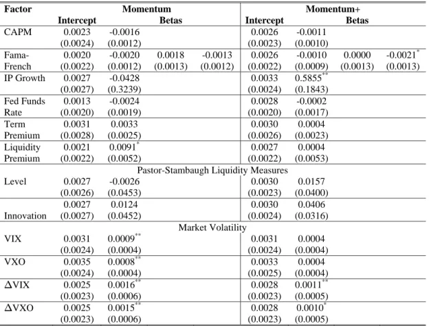
Factor Momentum Momentum+

Intercept Betas Intercept Betas CAPM 0.0023 (0.0024) -0.0016 (0.0012) 0.0026 (0.0023) -0.0011 (0.0010) Fama-French 0.0020 (0.0022) -0.0020 (0.0012) 0.0018 (0.0013) -0.0013 (0.0012) 0.0026 (0.0022) -0.0010 (0.0009) 0.0000 (0.0013) -0.0021* (0.0013) IP Growth 0.0027 (0.0027) -0.0428 (0.3239) 0.0033 (0.0024) 0.5855** (0.1843) Fed Funds Rate 0.0013 (0.0020) -0.0024 (0.0019) 0.0028 (0.0020) -0.0002 (0.0017) Term Premium 0.0031 (0.0028) 0.0033 (0.0025) 0.0030 (0.0026) 0.0004 (0.0023) Liquidity Premium 0.0021 (0.0022) 0.0091* (0.0052) 0.0027 (0.0022) 0.0004 (0.0053) Pastor-Stambaugh Liquidity Measures

Level 0.0027 (0.0026) -0.0026 (0.0453) 0.0030 (0.0023) 0.0157 (0.0400) Innovation 0.0027 (0.0027) 0.0124 (0.0452) 0.0030 (0.0024) 0.0406 (0.0316) Market Volatility VIX 0.0031 (0.0024) 0.0009** (0.0004) 0.0031 (0.0024) 0.0004 (0.0004) VXO 0.0035 (0.0024) 0.0008** (0.0004) 0.0033 (0.0025) 0.0004 (0.0004) ¢ ¢VIX 0.0025 (0.0023) 0.0016** (0.0006) 0.0028 (0.0023) 0.0011** (0.0005) ¢ ¢VXO 0.0025 (0.0023) 0.0015** (0.0006) 0.0028 (0.0023) 0.0010* (0.0005)

(24)

Table 8.Risk Factor Regressions

Out-of-sample risk-adjusted returns of equally weighted portfolios using the value strategy January 2004 – December 2008

Factor Value Value+

Intercept Betas Intercept Betas CAPM -0.0018 (0.0020) 0.0014** (0.0005) 0.0018 (0.0019) 0.0006 (0.0004) Fama-French -0.0017 (0.0020) 0.0015** (0.0006) -0.0003 (0.0010) 0.0008 (0.0010) 0.0019 (0.0018) 0.0009** (0.0004) -0.0011 (0.0011) -0.0011 (0.0011) IP Growth -0.0019 (0.0021) 0.3755* (0.2355) 0.0020 (0.0018) 0.5231** (0.2029) Fed Funds Rate -0.0020 (0.0021) 0.0002 (0.0016) 0.0024 (0.0019) 0.0013 (0.0010) Term Premium -0.0022 (0.0024) -0.0004 (0.0020) 0.0014 (0.0020) -0.0018 (0.0013) Liquidity Premium -0.0016 (0.0018) -0.0087** (0.0019) 0.0019 (0.0019) -0.0036** (0.0018) Pastor-Stambaugh Liquidity Measures

Level -0.0020 (0.0021) 0.0455** (0.0228) 0.0017 (0.0020) 0.0120 (0.0156) Innovation -0.0021 (0.0022) 0.0269 (0.0237) 0.0017 (0.0020) 0.0159 (0.0290) Market Volatility VIX -0.0026** (0.0018) -0.0008** (0.0001) 0.0015 (0.0019) -0.0003** (0.0001) VXO -0.0028** (0.0018) -0.0007** (0.0001) 0.0013 (0.0019) -0.0003** (0.0001) ¢ ¢VIX -0.0021 (0.0022) -0.0008 (0.0006) 0.0017 (0.0019) -0.0007** (0.0003) ¢ ¢VXO -0.0021 (0.0022) -0.0006 (0.0006) 0.0017 (0.0019) -0.0007** (0.0003)

(25)

Table 9.Risk Factor Regressions

Out-of-sample risk-adjusted returns of equally weighted portfolios using the VECM strategy January 2004 – December 2008

Factor VECM VECM+

Intercept Betas Intercept Betas CAPM 0.0020 (0.0022) -0.0019 (0.0012) 0.0025 (0.0017) -0.0005 (0.0004) Fama-French 0.0016 (0.0021) -0.0025** (0.0011) 0.0027** (0.0011) -0.0017 (0.0013) 0.0024 (0.0017) -0.0004 (0.0003) -0.0003 (0.0009) -0.0015 (0.0010) IP Growth 0.0024 (0.0027) -0.1011 (0.2417) 0.0026 (0.0017) 0.0011 (0.1504) Fed Funds Rate 0.0030 (0.0021) -0.0039** (0.0019) 0.0026 (0.0016) 0.0000 (0.0012) Term Premium 0.0031 (0.0028) 0.0044 (0.0027) 0.0025 (0.0018) -0.0003 (0.0016) Liquidity Premium 0.0019 (0.0022) 0.0098* (0.0053) 0.0025 (0.0017) 0.0021 (0.0022) Pastor-Stambaugh Liquidity Measures

Level 0.0023 (0.0026) -0.0310 (0.0392) 0.0026 (0.0017) 0.0180 (0.0186) Innovation 0.0024 (0.0027) -0.0194 (0.0377) 0.0026 (0.0017) 0.0179 (0.0269) Market Volatility VIX 0.0030 (0.0022) 0.0010** (0.0004) 0.0027 (0.0017) 0.0003 (0.0002) VXO 0.0033 (0.0023) 0.0009** (0.0003) 0.0028 (0.0017) 0.0002 (0.0002) ¢ ¢VIX 0.0023 (0.0025) 0.0012 (0.0010) 0.0026 (0.0017) 0.0001 (0.0002) ¢ ¢VXO 0.0024 (0.0025) 0.0010 (0.0009) 0.0026 (0.0017) 0.0002 (0.0002)

(26)

Second, in Tables 6–9, the correlation with the volatility measures serves only to eliminate alpha for the carry and value strategies; for momentum and VECM it serves to enhance alpha; thus the returns for these strategies still cannot be explained away. Moreover, the risk-factor explanation for returns completely evaporates for the momentum+ and VECM+ strategies (and to a large extent for the carry+ and value+ strategies as well). Out of the former two, momentum+ appears to have only some mild covariation with industrial production growth, whereas VECM+ appears to be uncorrelated with all the risk factors that we consider and in fact, the risk-adjusted returns shown in Table 9 (right panel alphas) are relatively constant and equal to the raw returns seen in Table 5 (3% per annum with a Sharpe Ratio of 0.69). Finally, although the alphas in Table 9 have wide standard errors, the point estimate is consistent with our no-risk-factor model, and the sample size is small, and we consider that our Giacomini-White and Correct Classification statistics (AUC and KS) provide the compelling out-of-sample evidence of unweighted- and return-weighted predictive ability against the null.

Thus our VECM+ (a CMV vector model augmented by information from the forward curve) appears to stand tallest among all the augmented carry models we have considered. It significantly beat a coin-toss as a directional forecast, its return-weighted performance also delivers statistically significant profits, its profits avoid negative skew, and they have no correlation with a standard set of risk factors.

6

Conclusion

This paper has presented new data and methods to explore an ongoing debate about the currency carry trade. We find that many widely-used carry trade strategies failed during the recent financial crisis, but those augmented by additional hedging signals have fared better. Building on prior work that identified the carry, momentum, and value (CMV) signals as jointly important (Jord`a and A. Taylor 2009), in this paper we also find a complementary role for information drawn from the forward yield curves (Ang and Chen, 2009; Clarida and M. Taylor 1997; and Clarida et al. 2009). When this full set of signals are employed, the resulting portfolios of trades are profitable, exhibit attractive Sharpe and skewness properties, and cannot be rationalized away using any standard risk factors.

(27)

Appendix

The list of sources we used to construct risk-factors is as follows:

• Fama-French Factors: Kenneth French data library

(http://mba.tuck.dartmouth.edu/pages/faculty/ken.french/data library.html)

• Industrial Production Growth: Federal Reserve Board release G.17

• Federal funds rate: Federal Reserve Board; Table H.15.

• Term Premium: Federal Reserve Board, Table H.15; 10-year T-Bill (Constant Maturity) less

3-month T-Bill (Secondary Market Rate).

• Liquidity Premium: Federal Reserve Board, Table H.15; 3-month Eurodollar rate less 3-month

T-Bill.

• Pastor and Stambaugh: Pastor website

(http://faculty.chicagobooth.edu/lubos.pastor/research/liq data 1962 2008.txt). • VIX:Yahoo! Finance.

• VXO:Yahoo! Finance.

References

Ang, Andrew and Joseph S. Chen. 2010. Yield Curve Predictors of Foreign Exchange Returns. U. C. Davis.mimeograph

Authers, John. 2010. Book extract: The Fearful Rise of Markets. The Financial Times May 21, 2010. Bacchetta, Philip, and Eric van Wincoop. 2006. Can Information Heterogeneity Explain the Exchange

Rate Determination Puzzle? American Economic Review 96(3): 552–76.

Bekaert, Geert, and Robert J. Hodrick. 1993. On Biases in the Measurement of Foreign Exchange Risk Premiums. Journal of International Money and Finance12(2): 115–38.

Brunnermeier, Markus K., Stefan Nagel, and Lasse H. Pedersen. 2008. Carry Trades and Currency Crashes. NBER Working Papers no. 14473.

Burnside, A. Craig, Martin Eichenbaum, Isaac Kleshchelski, and Sergio Rebelo. 2006. The Returns to Currency Speculation. NBER Working Papers no. 12489.

Burnside, A. Craig, Martin Eichenbaum, Isaac Kleshchelski, and Sergio Rebelo. 2008a. Do Peso Problems Explain the Returns to the Carry Trade? CEPR Discussion Papers no. 6873.

Burnside, A. Craig, Martin Eichenbaum, Isaac Kleshchelski, and Sergio Rebelo. 2008b. Do Peso Problems Explain the Returns to the Carry Trade? NBER Working Papers no. 14054.

Burnside, A. Craig, Martin Eichenbaum, and Sergio Rebelo. 2007. The Returns to Currency Speculation in Emerging Markets. NBER Working Papers no. 12916.

Burnside, A. Craig, Martin Eichenbaum and Sergio Rebelo. 2008. Carry Trade: The Gains of Diversifi-cation. Journal of the European Economic Association6(2-3): 581–88.

Chen, Yu-chin and Kwok Ping Tsang. 2009. What Does the Yield Curve Tell Us about Exchange Rate Predictability? University of Washington, Department of Economicsworking paper UWEC 2009-04. Cheung, Yin-Wong, Menzie D. Chinn, and Antonio Garcia Pascual. 2005. Empirical Exchange Rate Models of the Nineties: Are Any Fit to Survive? Journal of International Money and Finance 24(7): 1150–75.

(28)

Clarida, Richard H., Josh Davis and Niels Pedersen. 2009. Currency Carry Trade Regimes: Beyond the Fama Regression. Journal of International Money and Finance28(8): 1375–1389.

Clarida, Richard H., and Mark P. Taylor. 1997. The Term Structure Of Forward Exchange Premiums and the Forecastability of Spot Exchange Rates: Correcting the Errors. The Review of Economics

and Statistics79(3):353–361.

Clarida, Richard H., and Daniel Waldman. 2007. Is Bad News About Inflation Good News for the Exchange Rate? NBER Working Papers no. 13010.

Cochrane, John H. 2001Asset PricingNew Jersey: Princeton University Press.

Conover, W. J. 1999. Practical Nonparametric Statistics. 3rd edition. New York: John Wiley and Sons. Diebold, Francis X., and Roberto S. Mariano. 1995. Comparing Predictive Accuracy. Journal of Business

and Economic Statistics 13(3): 253–63.

Engel, Charles. 1996. The Forward Discount Anomaly and the Risk Premium: A Survey of Recent Evidence. Journal of Empirical Finance 3:123–191.

Fama, Eugene F. 1984. Forward and Spot Exchange Rates. Journal of Monetary Economics 14(3): 319–38.

Fama, Eugene F. and Kenneth R. French. 1993. Common Risk Factors in the Returns on Stocks and Bonds. Journal of Financial Economics 33: 3–56.

Fisher, Eric O’N. 2006. The Forward Premium in a Model with Heterogeneous Prior Beliefs. Journal of

International Money and Finance25(1): 48–70.

Frankel, Jeffrey A. 1980. Tests of Rational Expectations in the Forward Exchange Market. Southern

Economic Journal46(4): 1083–1101.

Froot, Kenneth A., and Richard H. Thaler. 1990. Foreign Exchange. Journal of Economic Perspectives

4(3): 179–92.

Giacomini, Raffaella, and Halbert White. 2006. Tests of Conditional Predictive Ability. Econometrica

74(6): 1545–78.

Hodrick, Robert J. 1987. The empirical evidence on the efficiency of forward and futures foreign exchange

markets. Chur: Harwood.

Hsieh, Fushing and Bruce W. Turnbull. 1996. Nonparametric and Semiparametric Estimation of the Receiver Operating Characteristics Curve. Annals of Statistics, 24: 25–40.

Ilut, Cosmin. 2008. Ambiguity Aversion: Implications for the Uncovered Interest Rate Parity Puzzle. Northwestern University. Photocopy.

Jeanne, Olivier, and Andrew K. Rose. 2002. Noise Trading And Exchange Rate Regimes. Quarterly

Journal of Economics 117(2): 537–69.

Jord`a, `Oscar, and Alan M. Taylor. 2009. The Carry Trade and Fundamentals: Nothing to Fear but FEER itself. NBER Working Papers no. 15518.

Jord`a, `Oscar, and Alan M. Taylor. 2010. Performance Evaluation for Zero Net-Investment Strategies. University of California, Davis, Photocopy.

Jurek, Jakub W. 2008. Crash-Neutral Currency Carry Trades. Princeton University. Photocopy. Kilian, Lutz, and Mark P. Taylor. 2003. Why is it so difficult to beat the random walk forecast of exchange

rates? Journal of International Economics 60(1): 85–107.

Meese, Richard A., and Kenneth Rogoff. 1983. Empirical Exchange Rate Models of the Seventies. Journal

of International Economics 14(1–2): 3–24.

Melvin, Michael, and Mark P. Taylor. 2009. The crisis in the foreign exchange market. Journal of

(29)

Nelson, Charles R. and Andrew F. Siegel. 1987. Parsimonious Modeling of Yield Curves. The Journal of

Business 60(4): 473-489.

Obuchowski, Nancy A. 1994. Computing Sample Size for Receiver Operating Characteristic Curve Studies.

Investigative Radiology, 29(2): 238–243.

Pastor, Lubos and Robert F. Stambaugh, 2003. Liquidity Risk and Expected Stock Returns. Journal of

Political Economy, vol. 111(3), pages 642–685, June.

Peirce, Charles S. 1884. The Numerical Measure of the Success of Predictions. Science 4: 453–454. Sarno, Lucio, and Mark P. Taylor. 2002. The Economics of Exchange Rates. Cambridge: Cambridge

University Press.

Shleifer, Andrei, and Robert W. Vishny. 1997. A Survey of Corporate Governance. Journal of Finance

52(2): 737–83.

Summers, Lawrence H. 1985. On Economics and Finance. The Journal of Finance 40(3): 633–635. Youden, W. J. 1950. Index for Rating Diagnostic Tests. Cancer 3, 32–35.