MODELING AND CONTROL OF AN ALTERNATING-CURRENT PHOTOVOLTAIC MODULE
BY
TRISHAN ESRAM
DISSERTATION
Submitted in partial fulfillment of the requirements
for the degree of Doctor of Philosophy in Electrical and Computer Engineering in the Graduate College of the
University of Illinois at Urbana-Champaign, 2010
Urbana, Illinois Doctoral Committee:
Associate Professor Patrick L. Chapman, Chair Professor Philip T. Krein
Professor Ty A. Newell Professor Peter W. Sauer
ABSTRACT
Energy independence depends greatly on the adoption of renewable energy sources. Yet, electricity, a commodity of everyday life, is currently being generated primarily from fossil fuels in the U.S. Despite the abundance of solar energy, the total electricity from photovoltaic (PV) sources is negligible, mainly because of the relatively high cost of PV systems. For PV electricity to become mainstream, its price has to reach grid parity, which is unachievable unless the overall cost of PV systems is reduced.
Alternating-current (ac) PV modules are shown to have the potential to significantly decrease the cost of PV systems. An ac PV module consists of an individual conventional PV module embodying a small inverter, often called a microinverter. AC PV modules provide simpler, faster, and less expensive installation. Unlike typical inverters,
microinverters are more reliable and robust and do not have to be replaced once or twice over the lifetime of the system. The flexibility provided by ac PV modules with
individual maximum power point tracking (MPPT) may also increase the energy yield. With several microinverters operating simultaneously in a PV system, as opposed to only one or two bigger inverter(s), it is of particular interest to investigate the behavior and dynamics of such a PV system and its compliance with regulatory codes and standards when interconnected with the utility grid. For this purpose, complete detailed ac PV module models, along with different possible control techniques, are developed, analyzed, and tested through simulations. Average-value models (AVMs) for the ac PV modules are shown to drastically reduce simulation times while preserving their
performances. The ac PV module AVMs therefore allow for rapid simulations and analyses of several ac PV modules running concurrently under numerous conditions.
I dedicate this dissertation to my mother, father, and brother.
ACKNOWLEDGMENTS
First of all, I would like thank my adviser, Professor Patrick L. Chapman. I remember clearly the first phone call I received from him, asking me whether I was still interested in joining the University of Illinois for my graduate studies under his supervision. It was a privilege for me to accept his offer and I spent the following several exceptional years learning from him and doing research with him. His advice, guidance, and help have always been invaluable. This dissertation is the outcome of the great collaboration between him and me. All this work would have been impossible without him.
I also remember my first meeting with Professor Chapman, at a time when he had just founded SmartSpark Energy Systems, Inc. He casually mentioned that maybe I could work for SmartSpark after graduation. Little did I know that this would indeed happen, although earlier than expected. I have been working for SmartSpark, now SolarBridge Technologies, Inc., for more than two years and much of the experience that I gained there is reflected in this dissertation. I would like to thank all my colleagues at SolarBridge for their support while I was finishing this dissertation.
I would also like to thank Professors Philip T. Krein and Robert S. Balog, whose research on the cycloconverter-type inverter instigated this dissertation on microinverter and ac PV module design. I have learned a considerable amount from Professor Krein’s classes, as both a student and a teaching assistant. Professor Balog’s time and patience in teaching me the cycloconverter operation will always be appreciated. I would like to thank Professors Peter W. Sauer and Ty A. Newell for being critics of this research from a different perspective than power electronics. I will never forget the amazing time I spent working with Professor Newell on the Solar Decathlon.
Most importantly, I would like to thank my parents, who have always been there for me. Their unconditional love and support have helped me surpass my own expectations. My brother has always known how to motivate me and push me beyond my limits; I thank him for that. Nora Wang, someone very special, has provided me with constant support, advice, ideas, and help throughout this dissertation work; I can never thank her enough for being there for me. I will forever be grateful to Rodney and Linda for their friendship. My thanks also go to the entire Power and Energy Systems group for hosting me for so many years and Jamie Hutchinson for editing this dissertation.
TABLE OF CONTENTS
Page
LIST OF FIGURES ... vii
LIST OF TABLES... xi
1 INTRODUCTION ...1
1.1 Overview... 1
1.2 Grid Parity... 2
1.3 AC PV Modules... 9
1.4 Initially Proposed Microinverter... 14
1.5 Alternative Microinverter ... 18
2 INPUT STAGE...20
2.1 Overview... 20
2.2 PV Module Model... 22
2.3 MPPT Algorithm ... 30
2.4 Boost Converter Setup for MPPT Analysis ... 35
2.5 Isolated Boost Converter... 43
2.6 Average-Value Model... 45 3 OUTPUT STAGE...47 3.1 Overview... 47 3.2 Abnormal Voltages ... 49 3.3 Abnormal Frequencies ... 50 3.4 Power Quality ... 50 3.5 Islanding... 51
3.6 Output Stage Simulations ... 62
3.7 Average-Value Model... 69 4 ENERGY STORAGE...73 4.1 Overview... 73 4.2 Passive Filter... 75 4.3 Active Filter ... 84 5 MULTI-INVERTER SYSTEM ...96 5.1 Overview... 96
5.2 Abnormal Grid Conditions ... 99
5.3 Islanding Detection in a PV System with Identical IDMs... 100
5.4 Islanding Detection in a PV System with Mixed IDMs ... 102
5.5 Power Quality ... 105
6 CONCLUSION...109
APPENDIX A CODES... 113
A.1 MATLAB Code for PV Data Extraction ... 113
A.2 Complete PV Module Model Modelica Code ... 114
A.3 dP-P&O MPPT Algorithm Modelica Code... 115
A.4 Modelica Code to Compute Root-Mean-Square (rms)... 117
A.5 Modelica Code to Compute Frequency ... 118
A.6 MATLAB Code to Perform FFT and Compute THD ... 118
A.7 Modelica Code for AFD IDM Current Command Generation... 119
A.8 Modelica Code for SMS IDM Current Command Generation... 120
A.9 Modelica Code for SFS IDM Current Command Generation ... 121
A.10 Modelica Code for Fault Detection... 122
APPENDIX B DERIVATIONS ... 124
B.1 Transfer Functions for Microinverter Input Stage ... 124
B.2 Transfer Functions for Microinverter with Passive Filter... 126
B.3 Transfer Functions for Microinverter with Active Filter... 128
APPENDIX C MULTIPLE-CARRIER PWM ... 131
LIST OF FIGURES
Page
Fig. 1.1 2008 U.S. electric power industry net generation [4]... 2
Fig. 1.2 Solar resources in Germany and the U.S., from [3] ... 3
Fig. 1.3 Electricity price peaking and irradiance on a typical summer day in Illinois ... 4
Fig. 1.4 2007 state electricity profile in ¢/kWh, from [8]... 5
Fig. 1.5 Variation in average installed cost among states, from [9] ... 5
Fig. 1.6 Variation in average installed cost based on PV system size, from [9]... 6
Fig. 1.7 2008 components of U.S. average electricity prices [10]... 6
Fig. 1.8 PV module prices (left) [11] and inverter prices (right) [12] ... 7
Fig. 1.9 Cost fractions from Table 1.2 [13] ... 8
Fig. 1.10 Setups for two different PV systems: PV system with string inverter (left) and PV system with ac PV modules (right) ... 10
Fig. 1.11 Additional power yielded by using ac PV modules instead of a string inverter ... 11
Fig. 1.12 Possible microinverter topologies as shown in [24]: (a) with line-frequency transformer and (b) with high-frequency transformer ... 12
Fig. 1.13 Classification of microinverters with high-frequency transformers [24]: microinverter with (a) dc link, (b) pseudo dc link, and (c) no dc link... 13
Fig. 1.14 Cycloconverter-type high-frequency link inverter proposed in [26]... 14
Fig. 1.15 State machine for cycloconverter control [27] ... 15
Fig. 1.16 Experimental waveforms and logic signals for initially proposed microinverter [27] ... 15
Fig. 1.17 Dymola simulation setup for initially proposed microinverter ... 16
Fig. 1.18 Simulation waveforms and logic signals from Dymola setup... 16
Fig. 1.19 Grid-tied cycloconverter-type inverter with PV source ... 17
Fig. 1.20 Waveforms with PV source and input filter ... 18
Fig. 1.21 Alternative microinverter with PV source and grid-tied ... 19
Fig. 2.1 Microinverter input stage... 20
Fig. 2.2 Example of characteristic i-v curve of a PV module ... 20
Fig. 2.3 Effects of insolation (left) and temperature (right) on a PV characteristic curve [30] ... 21
Fig. 2.4 PV module model ... 22
Fig. 2.5 Dymola PV module model block ... 29
Fig. 2.6 Voltage sweep simulation setup ... 29
Fig. 2.7 Good correlation between datasheet (left) [29] and simulated (right) i-v curves under varying T... 29
Fig. 2.8 i-v (left) and p-v (right) curves under varying insolation ... 30
Fig. 2.9 Slopes of PV module characteristic curve... 31
Fig. 2.10 Flowchart for basic P&O MPPT algorithm... 32
Fig. 2.11 Divergence of P&O under rapid insolation change... 33
Fig. 2.12 dP-P&O additional power measurement between two updates ... 33
Fig. 2.14 Dymola dP-P&O MPPT block... 35
Fig. 2.15 Boost converter connected to PV module ... 35
Fig. 2.16 Switching signal generation from MPPT duty ratio command ... 36
Fig. 2.17 Dymola setup to simulate MPPT with duty ratio command ... 36
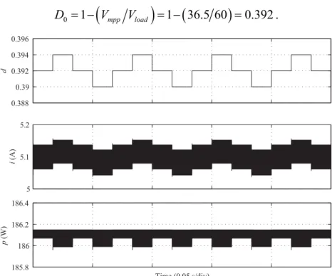
Fig. 2.18 Steady-state waveforms for MPPT with duty-ratio command ... 37
Fig. 2.19 120-Hz load disturbance transmitted to the input... 37
Fig. 2.20 Switching signal generation from MPPT current command ... 38
Fig. 2.21 Bandwidth of the input current control loop ... 38
Fig. 2.22 Bode plot of input current control loop ... 39
Fig. 2.23 Input transconductance ... 39
Fig. 2.24 Dymola setup to simulate MPPT with current command... 40
Fig. 2.25 Steady-state waveforms for MPPT with current command... 41
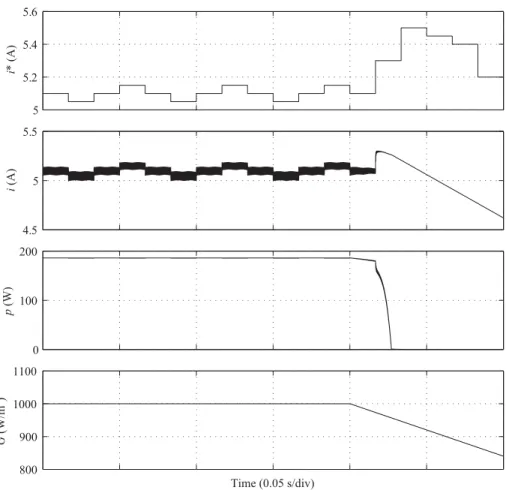
Fig. 2.26 Power collapse with MPPT current command under rapid decrease in insolation... 41
Fig. 2.27 Switching signal generation from MPPT voltage command... 42
Fig. 2.28 Alternative switching signal generation from MPPT voltage command ... 42
Fig. 2.29 Dymola setup to simulate MPPT with voltage command ... 42
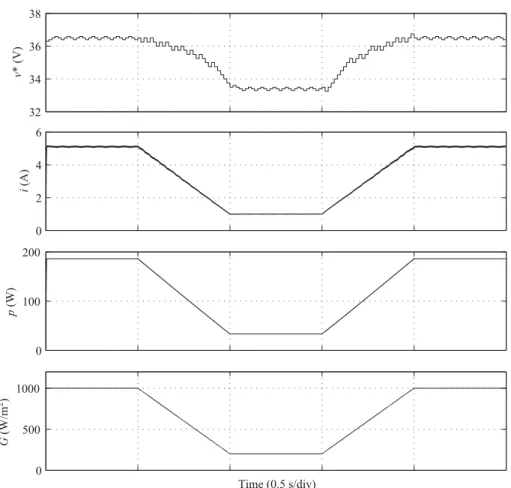
Fig. 2.30 Robustness of control scheme using MPPT with voltage command under varying insolation... 43
Fig. 2.31 Switching signals for input full-bridge inverter ... 44
Fig. 2.32 Dymola microinverter input stage setup... 45
Fig. 2.33 Dymola average-value model for input converter... 45
Fig. 2.34 Dymola setup with boost converter average-value model... 46
Fig. 2.35 Waveforms from boost converter average-value model setup ... 46
Fig. 3.1 Microinverter output stage... 47
Fig. 3.2 Common grid-tied PV system interconnection as shown in [41]... 47
Fig. 3.3 Dymola root-mean-square (rms) computation block... 49
Fig. 3.4 Dymola frequency computation block ... 50
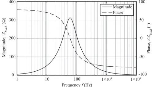
Fig. 3.5 Magnitude and phase of an example parallel RLC load... 53
Fig. 3.6 Nondetection zone for UFP/OFP... 54
Fig. 3.7 AFD current waveform and its fundamental with respect to voltage waveform ... 55
Fig. 3.8 Nondetection zone for AFD ... 57
Fig. 3.9 Intersections of load lines and disturbance functions... 58
Fig. 3.10 Nondetection zone for SMS ... 59
Fig. 3.11 Nondetection zone for SFS... 61
Fig. 3.12 Dymola block for IDM current command generation ... 62
Fig. 3.13 Dymola setup to simulate output stage... 62
Fig. 3.14 iout and i* when δf = 1.5 Hz with AFD IDM ... 64
Fig. 3.15 Harmonic content of iout when δf = 1.5 Hz with AFD IDM ... 64
Fig. 3.16 AFD islanding detection when δf = 1.5 Hz, Qf = 1.0, and f0 = 60 Hz ... 65
Fig. 3.17 AFD islanding nondetection when δf = 1.5 Hz, Qf = 3.0, and f0 = 60 Hz ... 66
Fig. 3.18 iout and i* when θm = 10° with SMS IDM ... 66
Fig. 3.19 Harmonic content of iout when θm = 10° with SMS IDM ... 67
Fig. 3.21 SMS islanding nondetection when θm = 10°, Qf = 3.0, and f0 = 60 Hz ... 68
Fig. 3.22 SFS islanding detection when k = 0.05, δf0 = 1.5 Hz, Qf = 1.0, and f0 = 60 Hz ... 68
Fig. 3.23 SFS islanding nondetection when k = 0.05, δf0 = 1.5 Hz, Qf = 3.0, and f0 = 59.6 Hz ... 69
Fig. 3.24 Dymola average-value model for output full-bridge inverter ... 70
Fig. 3.25 Dymola output stage setup using output full-bridge AVM ... 70
Fig. 3.26 AFD islanding detection with AVM when δf = 1.5 Hz, Qf = 1.0, and f0 = 60 Hz ... 71
Fig. 3.27 SMS islanding detection with AVM when θm = 10°, Qf = 1.0, and f0 = 60 Hz ... 71
Fig. 3.28 SFS islanding detection with AVM when k = 0.05, δf0 = 1.5 Hz, Qf = 1.0, and f0 = 60 Hz ... 72
Fig. 4.1 AC PV module connected to the utility grid ... 73
Fig. 4.2 Microinverter instantaneous output power ... 74
Fig. 4.3 Double-frequency power ... 74
Fig. 4.4 Double-frequency energy ... 75
Fig. 4.5 Control topology for passive filter... 77
Fig. 4.6 Bandwidth of bus voltage control loop... 78
Fig. 4.7 Bode plot of bus voltage control loop gain... 78
Fig. 4.8 Effective bus impedance... 79
Fig. 4.9 Dymola setup for grid-tied ac PV module with passive filter ... 80
Fig. 4.10 Simulation waveforms of grid-tied ac PV module with passive filter ... 81
Fig. 4.11 Simulation waveforms of average-value model of ac PV module with passive filter ... 82
Fig. 4.12 Average-value model of ac PV module with passive filter ... 83
Fig. 4.13 Waveforms under rapid insolation changes for ac PV module with passive filter... 84
Fig. 4.14 Energy variation in passive filter... 85
Fig. 4.15 Active filter converter... 86
Fig. 4.16 Ideal active filter waveforms ... 86
Fig. 4.17 Waveforms resulting from energy offset... 87
Fig. 4.18 Control topology for active filter, based on [56] ... 88
Fig. 4.19 Bandwidth of bus voltage control loop... 89
Fig. 4.20 Bode plot of bus voltage control loop gain... 89
Fig. 4.21 Bandwidth of active filter voltage control loop... 90
Fig. 4.22 Bode plot of active filter voltage control loop gain... 90
Fig. 4.23 Effective bus impedance in the presence of active filter ... 90
Fig. 4.24 Simulation waveforms of grid-tied ac PV module with active filter... 91
Fig. 4.25 Dymola setup for grid-tied ac PV module with active filter ... 92
Fig. 4.26 Simulation waveforms of average-value model of ac PV module with active filter... 93
Fig. 4.27 Average-value model of ac PV module with active filter ... 94
Fig. 4.28 Waveforms under rapid insolation changes for ac PV module with active filter... 95
Fig. 5.1 PV system with multiple ac PV modules ... 97 Fig. 5.2 Dymola ac PV module blocks ... 98 Fig. 5.3 Dymola setup to simulate PV system with multiple ac PV modules ... 98 Fig. 5.4 Shutdown of a PV system with 10 ac PV modules due to abnormal grid
voltage... 99 Fig. 5.5 Shutdown of a PV system with 10 ac PV modules due to abnormal grid
frequency... 100 Fig. 5.6 Islanding detection in a PV system of 10 ac PV modules with AFD... 100 Fig. 5.7 Islanding detection time for different combinations of ac PV modules with
AFD and SMS... 103 Fig. 5.8 Islanding detection time for different combinations of ac PV modules with
AFD and SFS ... 104 Fig. 5.9 Islanding detection time for different combinations of ac PV modules with
SFS and SMS ... 105 Fig. 5.10 PWM switching signals generation for the output full-bridge converter ... 106 Fig. 5.11 Current iPV with synchronized carrier signals... 107
Fig. 5.12 Harmonics around switching frequency with synchronized carrier signals ... 107 Fig. 5.13 Carrier signals 90° out of phase from each other ... 108 Fig. 5.14 Current iPV with unsynchronized carrier signals... 108
Fig. 5.15 Harmonics around switching frequency with unsynchronized carrier
signals ... 108 Fig. C.1 Example of multiple-carrier PWM generation ... 132 Fig. C.2 Two methods of generating the same gate control sequence... 133
LIST OF TABLES
Page
Table 1.1 Electricity generation costs [5] ... 3
Table 1.2 Cost breakdown for installed residential PV system in 2008 [13] ... 8
Table 2.1 Simulated MPP datapoints vs. insolation levels ... 30
Table 3.1 Interconnection system response to abnormal voltages [42] ... 49
Table 3.2 Interconnection system response to abnormal frequencies [42]... 50
Table 3.3 Maximum harmonic current distortion in percent of current [42]... 51
Table 4.1 Microinverter and control parameter settings... 79
Table 5.1 Islanding detection time versus number of ac PV modules, at 1000 W/m2 and 25 °C ... 101
Table 5.2 Islanding detection time versus insolation, with 10 ac PV modules at 25 °C ... 102
Table 5.3 Islanding detection time for different combinations of ac PV modules with AFD and SMS... 102
Table 5.4 Islanding detection time for different combinations of ac PV modules with AFD and SFS ... 104
Table 5.5 Islanding detection time for different combinations of ac PV modules with SFS and SMS ... 105
1 INTRODUCTION 1.1 Overview
With the soaring prices and scarcity of fossil fuels, the pursuit of energy
independence, and the growing concern about carbon emissions, solar energy is showing great potential. Consequently, producing electricity from photovoltaic (PV) systems is becoming more feasible. Yet, for PV electricity to become mainstream, grid parity—the point at which PV resources become competitive with more conventional electrical resources [1]—has to be reached. In Section 1.2, different views of grid parity will be discussed. Regardless of the type of parity, cheaper and more efficient solar cell
technologies, cheaper and more reliable inverters, cheaper and easier installation, better governmental policies and incentives, and better green public education are required to bring down PV system costs, which, in turn, can lower the cost of PV electricity.
Alternating-current (ac) PV modules, though not currently on the market, can help achieve several of these requirements. An ac PV module consists of an individual conventional PV module embodying a relatively small inverter, often called a
microinverter. The different aspects of ac PV modules will be covered in Section 1.3, along with a review of possible microinverter topologies. While microinverters serve the same purpose as bigger string or central inverters that are connected to strings or arrays of PV modules—conversion of direct-current (dc) power from PV modules into ac power—they represent a couple of challenges. Attached to the back of PV modules, microinverters have to be not only compact and light, but also reliable enough to match or outlast the common 20–25-year lifetime of the PV modules.
A cycloconverter-type inverter topology showed the potential to meet these
challenges and was thus initially proposed for this research work. However, as discussed in Section 1.4, upon further investigation of this inverter topology in the context of ac PV modules, several limitations arose in terms of controls and component sizes, making it less suitable to be incorporated into ac PV modules.
A topology consisting of an isolated boost converter input stage and a full-bridge inverter output stage is therefore proposed in Section 1.5 for the microinverter. In the subsequent chapters, this microinverter, along with necessary controls for its two stages, will be developed, modeled, and tested through simulations. Combined with a model of a
PV module, the microinverter and its controls will form a complete ac PV module model. The performance of the ac PV module model will also be evaluated via simulations. Several ac PV modules in parallel on the same circuit—representative of a typical PV system—connected to the ac utility grid will be simulated to investigate the interaction of microinverters with the grid and verify compliance with regulatory codes and standards. The ac PV module model will be a useful tool for future development of PV systems.
1.2 Grid Parity
1.2.1 Photovoltaic in the Electricity Market
The abundance of solar energy is indisputable. According to [2], the sun provides four orders of magnitude more power than the 13 terawatts (TW) consumed by the world, and only about 4 gigawatts (GW)—or about four orders of magnitude less than the
world’s power consumption—of photovoltaic is installed across the world. In other words, solar energy is being underutilized and there is plenty of room for PV systems to penetrate the electricity market.
According to a 2007 PV market survey, “the U.S. solar energy industry saw a glimpse of a gigawatt future”—the point at which contribution to the overall electricity production becomes significant and noticeable [3]. However, in 2008, less than 1% of the electricity generated in the U.S. was from solar power, based on data from the U.S. Energy
Information Administration (EIA). The remainder was dominated by fossil fuel and nuclear sources, as can be seen in Fig. 1.1, which shows the breakdown of the U.S. electric power industry net generation in 2008 [4].
Coal 48.2% Petroleum 1.1% Natural Gas 21.4% Nuclear 19.6% Other Gases 0.3% Other 0.3% Hydroelectric 6.0% Other Renewables 3.1%
Although its PV installations and production have been increasing at a steady rate, the U.S. is only the fourth largest PV market in the world, behind Germany, Japan, and Spain [3]. Ironically, when compared to Germany, solar resources are considerably higher in the U.S., as shown in Fig. 1.2. The U.S. clearly has all the required resources for solar energy to be a major contributor to the electricity market, but the cost of generating electricity from PV systems has remained high, making grid parity difficult to achieve.
Fig. 1.2 Solar resources in Germany and the U.S., from [3]
Table 1.1 [5] gives a general idea of the present costs of generating electricity from several sources and confirms that PV electricity costs are an order of magnitude higher than those of base load generation sources such as coal. It is worth noting that electricity costs from distributed PV systems (like residential rooftop systems) tend to be higher than centralized PV systems (like utility-scale systems). As can also be noted, wind energy is on par with the base load sources, hence its successful integration in the electricity market.
Table 1.1 Electricity generation costs [5]
Source ¢/kWh
Coal integrated gas combined cycle (IGCC) 3–5
Wind 4–7
Biomass gasification 7–9
Remote diesel generation 20–40
PV central station 20–30
Which one or combination of the sources is used to generate electricity depends on the market demand, which varies continuously throughout the day and year. As a result, there are several different kinds of grid parity: spot market, peak, retail, and cost parity [1]. While spot market parity is the easiest to achieve by the cost of PV energy matching or falling below the locational marginal price (LMP) of a given area, the very rare occurrence of high LMPs makes it the least useful [1].
1.2.2 Peak Parity
Peak parity, on the other hand, is considered as being the point at which PV electricity cost matches or falls below generation costs from conventional peaking
sources such as diesel generators. Peak parity is more viable not only because the costs of producing electricity on a large scale from PV and diesel are already in the same range (see Table 1.1), but also because solar energy tends to be most readily available at the times of peak demand. This is evident from Fig. 1.3, which shows the solar irradiance recorded on a typical summer day in Illinois [6] along with the electricity real time price (RTP) for that same day [7].
0.02 0.04 0.06 0.08 0 4 8 12 16 20 24 0 200 400 600 800 1000 Hour (CST) Irradiance (W/m 2)
Real Time Price ($/kWh)
Fig. 1.3 Electricity price peaking and irradiance on a typical summer day in Illinois 1.2.3 Retail Parity
When PV electricity cost at the point of end use equals or drops below the average retail cost at a given location, retail parity is reached—this is the usual definition of grid parity [1]. However, since average electricity prices vary from state to state as reported by the EIA [8] and shown in Fig. 1.4, for a given PV system cost, retail parity cannot be
achieved simultaneously nationwide. This is further accentuated by the fact that, based on 37,000 PV system installations throughout the country, [9] reported that the average installed cost of PV systems varies not only across states, as shown in Fig. 1.5, but also with size as in Fig. 1.6. These result from bigger systems benefitting from economy of scale and states having different policies, incentives, and cost of labor, among several factors affecting the cost of PV systems.
Fig. 1.4 2007 state electricity profile in ¢/kWh, from [8]
Fig. 1.6 Variation in average installed cost based on PV system size, from [9]
In Figs. 1.5 and 1.6, “n” represents the number of installations in each category. It is interesting to see in Fig. 1.5 that California and New Jersey have the most PV system installations—the positive consequence of their better policies and attractive incentives. Even more interesting in Fig. 1.6 is that most of the installations are in the 2–5-kW range, which usually corresponds to residential-scale systems. For residential rooftop
installations, PV electricity has to compete with the retail electricity prices, which include distribution and transmission fees. According to the EIA [10], these usually accounted for about 31% of the price in 2008, as shown by the distribution in Fig. 1.7. Therefore, even though Table 1.1 indicates higher electricity prices for distributed PV systems, they should not be compared to the other sources without including the distribution and transmission fees. This also indicates that, although more costly to install, smaller PV systems might reach grid parity concurrently with or even sooner than larger ones.
Generation 69% Distribution 24% Transmission 7%
1.2.4 Cost Parity
Probably the most difficult to reach, cost parity is when the cost of PV electricity is less than or equal to wholesale electricity rates or even dominant base load rates for a given region [1]. Achieving cost parity implies that PV sources are able to successfully compete with other energy sources, thus increasing the initiatives to proliferate the use of solar energy. As mentioned above, electricity from wind energy is very close to cost parity, as witnessed by its strong presence in the U.S. and many other countries. 1.2.5 Implications
Based on peak, retail, and wholesale rates in typical U.S. locations and the amount of energy that a conventional PV cell can produce over its lifetime at a typical location in North America, [1] estimated that peak, retail, and cost parity can be reached if the initial installed cost of a complete unsubsidized PV system is about $4.38, $2.63, and $1.10 per peak watt, respectively. According to Solarbuzz, as of March 2010, the average retail prices are about $4.24 per watt for PV modules [11] and $0.72 per watt for inverters [12], resulting in a total of $4.96 per watt. This is already above the peak parity cost and does not even include installation costs. In Fig. 1.8, it is interesting to note that PV module prices showed some decline in the past year, unlike inverter prices.
4.2 4.3 4.4 4.5 4.6 4.7 4.8 4.9 Jan-07 Ma y-07 S ep-07 Jan-08 Ma y-08 Se p-08 Jan-09 Ma y-09 S ep-09 Ja n-10 P V mo d u le p ric e ( $ /W ) 0.6 0.65 0.7 0.75 0.8 Oct-08D ec-08 Fe b-09 Ap r-09 Ju n-09 Aug -09 Oct-09D ec-09 Fe b-10 In ve rt e r p ri c e ( $ /W )
Fig. 1.8 PV module prices (left) [11] and inverter prices (right) [12]
A more comprehensive breakdown of the initial cost of installing a PV system in 2008 is given in Table 1.2, using data from [13]. The total amounts to $8.25 per watt. While the costs are somewhat optimistic when compared to those in Fig. 1.8, the relative values are instructive. The percentages of the breakdown are shown in Fig. 1.9 and are
representative of systems in the range of 2 to 5 kW—larger systems have a different relative mix. As can be seen, manufacturing the PV cells and assembling them into modules represent about 45% of the total cost. The remainder is divided among the installation of the system, inverters, and other hardware components. It is interesting to see that installation accounts for 40% of the price. It also has to be pointed out that, even though the inverters represent only about 6% of the up-front total price, they usually have to be replaced once or twice over the lifetime of the PV system since the mean time between failures (MTBF) of an inverter is from 5 to 10 years, while the MTBF of most PV modules is about 25 years. This further increases the contribution from inverters [1].
Table 1.2 Cost breakdown for installed residential PV system in 2008 [13]
Sector Cost ($/W)
Polysilicon 1.50 Wafers from polysilicon 0.75
PV cells from wafers 0.75 Completion of PV modules 0.75 Inverters 0.50 Other components 0.75 Installer's labor 1.25 Installer's overhead 2.00 Total 8.25 Polysilicon 18%
PV cells from wafers 9% Completion of PV modules 9% Inverters 6% Other components 9% Installer's labor 15% Installer's overhead 25% Wafers from polysilicon 9%
Fig. 1.9 Cost fractions from Table 1.2 [13]
There seems to be a misconception that lowering the cost of PV modules alone can lead to grid parity [14]. Clearly, to achieve any one type of grid parity, the overall cost of PV systems has to be brought down by decreasing the cost of every sector in Fig. 1.9. As will be discussed hereinafter, the use of ac PV modules has the potential to cut the costs of all the sectors except those related to the manufacturing of PV modules.
1.3 AC PV Modules
1.3.1 Simpler and Less Expensive Installation
Clause 690.2 of the 2008 National Electrical Code (NEC) [15] defines an ac PV module as “a complete, environmentally protected unit consisting of solar cells, optics, inverter, and other components, exclusive of tracker, designed to generate ac power when exposed to sunlight.” In other words, unlike regular PV modules, ac PV modules do not have any accessible dc circuits, and none of the dc code requirements in Section 690 of the NEC apply [16]. This definition also implies that ac PV modules are listed as unified devices consisting of small inverters attached permanently to the back of conventional PV modules [16]. As mentioned in [16], the interconnections of separately listed small inverters and PV modules do not qualify as an ac PV module, and requirements are imposed on dc wire size, dc overcurrent protection, and ground fault interruption, as per the NEC. Equipment grounding of the PV module frame can also be done through the integrated inverter, thus eliminating the need to run a separate equipment-grounding conductor, as is commonly the case in a typical PV system.
With the modular aspect of ac PV modules, power mismatch among PV modules is not problematic because they work independently of each other, with individual
maximum power point tracking (MPPT) [17, 18]. Since there is no need to match the voltage and current ratings of the PV modules, PV systems can easily incorporate different PV modules—either of the same model with widely varying tolerances, different models from the same manufacturer, or from different manufacturers. Unlike systems with string or central inverters, systems with ac PV modules do not have to enforce precision and consistency in mounting the PV modules to ensure maximum energy yield. As a result, simpler mounting hardware/components can be used, making the installation process easier, faster, and less expensive.
1.3.2 Extended Inverter Lifetime
As pointed out above, the inverter attached permanently to the back of the PV module is an inherent feature of an ac PV module. As such, unlike string and central inverters that only last 5 to 10 years, inverters for ac PV modules must be reliable enough to match or outlast the common 20–25-year lifetime of the PV modules. Conventional inverters
usually suffer from poor reliability because of their use of low-cost aluminum electrolytic capacitors for internal energy storage. These capacitors have limited life that is difficult to extend even with derating strategies [1]. Film capacitors or ceramic capacitors are known to be more reliable, but are far more expensive for the same capacitance. Nevertheless, [19] employs an active filter technique that uses less capacitance to store the same amount of energy, thus making the use of film or ceramic capacitors feasible and providing inverters with the reliability levels needed to support 25-year life. This active filter technique is analyzed in Chapter 4. Therefore, without the need to replace inverters once or twice, the lifetime cost of a PV system will be reduced.
1.3.3 Better Energy Yield and System Reliability
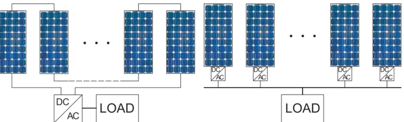
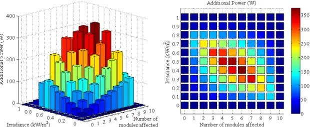
Complete or partial shadowing of one or more of the ac PV modules in a PV system only affects the energy yield of the respective module(s) and not the entire PV system. To better illustrate the improvement in power output by using ac PV modules, two systems were simulated, each representative of a typical 2-kW system, having ten 185-W PV modules. One of the systems uses a standard string inverter with the PV modules connected in series and MPPT performed on the entire string. The other system uses ac PV modules, with individual MPPT, connected in parallel. The setups for these two systems are shown in Fig. 1.10. For each system, the number of modules affected by shadowing is incremented and, for each case, the irradiance level is varied from 1 kW/m2 (full sun) to 0 kW/m2 (no sun) and the power delivered to the load is recorded. The additional power that can be obtained by using ac PV modules is then computed. The outcome in Fig. 1.11 shows that, in the best case, a system with ac PV modules can yield more than an additional 350 W.
DC AC DC AC DC AC DCAC DCAC
. . .
. . .
LOAD
LOAD
Fig. 1.10 Setups for two different PV systems: PV system with string inverter (left) and PV system with ac PV modules (right)
Fig. 1.11 Additional power yielded by using ac PV modules instead of a string inverter
Another limitation of centralized or string inverters is that all the PV modules have to be at the same tilt angle in order to prevent power mismatch. As mentioned previously, this is not a problem for ac PV modules, and they can thus be more easily adapted to odd roof-lines with different tilt angles and orientations, without considerably compromising the overall power output of the PV system. More importantly, better system reliability is achieved with the modularity of ac PV modules. If one of the modules is lost due to some failure in each system, the string inverter system is completely brought down while the modular system remains functional as the ac PV modules continue to supply power to the load. Moreover, the use of ac PV modules eliminates the need for special, properly sized dc cables that carry high currents at lower voltages, thus simplifying system design and improving system efficiency by eliminating dc losses.
1.3.4 Microinverter Topologies for AC PV Modules
Although ac PV modules are not currently available on the market, they have been the subject of much research, development, and attempted market penetration over the past couple of decades [20-22]. Ascension Technology, Inc., started development of ac PV modules in 1991 [21] and started shipping them in 1997 [23]. In 1995, OKE-Services developed microinverters [20], which were integrated on PV modules and shipped by NKF Kabel B.V. in 1996 [23]. However, supply of these ac PV modules on the market was short-lived—Applied Power Corporation bought Ascension Technology and discontinued its ac PV module line in 2001 and NKF Kabel stopped production of the microinverters in 2003 when a Dutch subsidy program ended [23].
In 2006, researchers in [22] claimed to be very close to having a fully operational ac PV module, but only presented a prototype, which required further development to reach the performance of string and central inverters; there has not been any update since then. On the other hand, there are companies such as Enphase Energy and Petra Solar that are currently marketing microinverters, which are only warranted for up to 15 years. As a result, they are not directly attached to PV modules, have exposed dc wiring, and do not qualify as ac PV modules. It is apparent that ac PV modules are not realizable unless reliability of the microinverters can match that of PV modules—this is highly dependent on the circuit topology of the microinverters.
References [24] and [25] have reviewed most of the ac PV module microinverter topologies that have been used in commercial ac PV modules and introduced in the literature. Since the majority of PV modules on the market output low dc voltage, the basic requirement for microinverters is to provide voltage amplification and dc–ac inversion in their power conversion stage [24]. Generally, voltage amplification can be realized by using either a line-frequency transformer or a high-frequency transformer as shown in Fig. 1.12. PV Module DC–AC Inverter Line Frequency Transformer Grid (a) Converter 2 High Frequency Transformer Converter 1 (b)
Fig. 1.12 Possible microinverter topologies as shown in [24]: (a) with line-frequency transformer and (b) with high-frequency transformer
In Fig. 1.12 (a), voltage amplification by the line-frequency transformer is preceded by a dc–ac inversion stage. Since a microinverter is an integral part of the assembly in an ac PV module, compactness is desired, meaning that a high power density is important [24]. However, line-frequency transformers tend to be bulky and may not be very
efficient. Interestingly, this was the topology employed by Ascension Technology for its ac PV module [21]. For the reasons above, microinverters with high-frequency
transformers are preferred. Depending on the configuration of Converter 2 in Fig. 1.12 (b), microinverters with high-frequency transformers can be classified as having either a dc link, a pseudo dc link, or no dc link, as shown in Fig. 1.13 (a), (b), and (c),
DC–AC Inverter HF Transformer DC Link DC–DC Converter (a) Line Frequency Unfolder HF Transformer DC–DC Converter (b) Cycloconverter HF Transformer (c)
Fig. 1.13 Classification of microinverters with high-frequency transformers [24]: microinverter with (a) dc link, (b) pseudo dc link, and (c) no dc link
In Fig. 1.13 (a), the input converter, the high-frequency transformer, and the rectifier form a dc–dc converter, which is basically an isolated boost converter that amplifies the low dc voltage from the PV module to a higher dc voltage for the dc link, before the dc– ac inversion takes place. The dc–dc converter in the pseudo dc link microinverter in Fig. 1.13 (b) is slightly different, in that it is modulated to provide a rectified sinusoidal voltage to the output stage, where it is unfolded to match the grid voltage. The third configuration does not include any dc link. The input stage converts the dc voltage from the PV module to a high-frequency square wave. After the square wave is amplified by the high-frequency transformer, an ac–ac converter (cycloconverter) is used to
reconstruct a sinusoidal voltage or current waveform at the line frequency.
While there are very many different commercial and experimental circuits, as shown in [24] and [25], that can be categorized as one of the above topologies, for the sake of brevity of this document, they will not be individually addressed and analyzed here. Nevertheless, the authors in [24] strongly believe that the microinverter topology without a dc link “may become the trend for the development of the next generation” of
microinverters. One major advantage of this topology over the other high-frequency transformer topologies is that there are only two power conversion stages. This implies that there is the possibility for fewer components, higher reliability, better efficiency, and lower overall cost. However, the authors in [24] find constructing bidirectional switches needed for the output converter to be a challenge and claim that more sophisticated controls are needed due to the loss of an intermediate energy storage stage.
1.4 Initially Proposed Microinverter
The cycloconverter-type high-frequency link inverter, proposed in [26] and shown in Fig. 1.14, was initially introduced and intended for fuel cell applications. Yet, this topology is very much like that shown in Fig. 1.13 (c), with a typical full-bridge inverter at the input to generate a high-frequency square wave, a high-frequency transformer to amplify the square wave, and a cycloconverter at the output to generate a line-frequency sinusoidal wave. At first glance, this particular topology seems to lend itself well to an ac PV module microinverter. Moreover, it resolves the challenges of constructing
bidirectional switches and eliminates the need for more complex controls, as mentioned at the end of Section 1.3.4. The bidirectional switches for the cycloconverter are
implemented with anti-parallel thyristors, which are controlled by a state machine.
Full-Bridge Transformer Cycloconverter
Q11 Q12 Q21 Q22 vload + _ iload v HF + _ vin + _ iin Q1 Q7 Q5 Q3 Q6 Q4 Q2 Q8
Fig. 1.14 Cycloconverter-type high-frequency link inverter proposed in [26]
The state machine in Fig. 1.15 was introduced and analyzed in [27], where it was shown to solve the cycloconverter-related issue of current commutation by generating switching signals to turn on the appropriate pairs of thyristors at the appropriate time. According to [27], while the load current changes sign, “improper switching can cause commutation failure where either the source is short-circuited or the load current is interrupted”—situations capable of causing high current or voltage that can damage the circuit. There are only four allowable states in the state machine. Depending on HFPOL, the polarity of the high-frequency voltage square wave vHF, and IP and IN, the load
current iload polarity signals based on some fixed thresholds, the state machine moves
from one state to another and outputs the switching signals to turn on the appropriate pair of thyristors. These switching signals are governed by the delay (DE) and advance (AD) pulse width modulation (PWM) signals, obtained from a multiple-carrier PWM technique covered in [26].
Q1 Q2 Q7 Q8 Q3 Q4 Q5 Q6 delay (HFPOL,IP,IN) advance
(0,0,0) (1,0,0) (1,0,1) (0,0,1) (1,0,0) (0,0,0) (0,1,0) (1,1,0) v HF: P→N i load: P→N vHF: P→N iload: N→P vHF: N→P iload: N→P vHF: N→P iload: P→N vHF: N→P vHF: N→P vHF: P→N vHF: P→N (DE) (AD)
Fig. 1.15 State machine for cycloconverter control [27] 1.4.1 Hardware Implementation
The authors in [27] implemented the inverter, along with the state machine, in hardware. A 30-V dc voltage supply was used as the input source and a 6.2-Ω resistor R
in series with a 35-mH inductor L as the load, with a switching frequency of 1 kHz. Figure 1.16 shows the waveforms and logic signals recorded from their experiment. The current iload is sinusoidal at the line frequency, although there is some low-frequency
distortion. The conversion from a high-frequency square wave to a low-frequency sinusoid can be clearly noted. It is also interesting to see how the DE and AD pulses are steered based on HFPOL, IP, and IN to generate the switching signals for the thyristors.
Q7|Q8 Q5|Q6 Q3|Q4 Q1|Q2 IN IP HFPOL AD DE Time (5 ms/div) iload vHF
1.4.2 Simulation
The hardware results being promising, for further tests and observations, the
cycloconverter-type inverter was modeled in Dymola [28], as illustrated in Fig. 1.17. The control block implements the state machine and generates all the switching signals. The model was simulated using the same settings as the hardware implementation, but with ideal components. The simulated waveforms and logic signals are shown in Fig. 1.18. The logic signals are practically similar to those shown in Fig. 1.16. In the absence of non-ideal components, iload is much cleaner, with no apparent low-frequency distortion
and no commutation failure. The load voltage vload is shown here, instead of vHF, to show
how vHF is modulated by the cycloconverter to produce a PWM voltage across the load.
The low line-frequency content of this PWM voltage is easily separated and recovered from its high-frequency switching content by the low-pass characteristic of the R-L load.
Fig. 1.17 Dymola simulation setup for initially proposed microinverter
Q7|Q8 Q5|Q6 Q3|Q4 Q1|Q2 IN IP HFPOL AD DE iload (A) vload (V) Time (5 ms/div) 0 0 80 −80 3.6 −3.6
1.4.3 Limitations
To test the feasibility of using the cycloconverter-type inverter as the microinverter of a grid-connected ac PV module, it needs to be simulated with a PV module as its source and the ac grid as its load. One example of doing this is shown in Fig. 1.19, where Lin and
Cin form an input filter and Lout an output filter. There are other possible configurations,
but this one is probably the simplest. Capacitor Cin also serves as the energy storage of
the energy flowing to and from the ac load at double its frequency.
Q11 Q12 Q21 Q22 v load + _ iload v HF + _ v in + _ iin Q1 Q7 Q5 Q3 Q6 Q4 Q2 Q8 PV L in Cin v i + _ Lout v grid
Fig. 1.19 Grid-tied cycloconverter-type inverter with PV source
The goal of a microinverter is to deliver the maximum available power from the PV module to the ac grid while meeting all the regulatory codes and standards, which are discussed in detail in Chapter 3. The current iload injected in the ac grid has to meet
well-defined harmonic limits and is usually desired to be in phase with grid voltage vgrid for
unity power factor. However, simulations showed that the setup in Fig. 1.19 can get close to meeting these requirements only at the expense of excessively big, maybe unrealistic, passive components.
For example, with a BP 7185 [29] 185-W PV module model, 240-V grid voltage, and the switching frequency increased to 4 kHz, Lin, Cin, and Lout had to be set at 1 mH,
1600 μF, and 342 mH, respectively, to generate the waveforms shown in Fig. 1.20. At a relatively low input voltage, a high capacitance is needed for Cin to manage the
double-frequency energy, while minimizing the variation in the voltage vin. Along with Cin, Lin is
sized to form a low-pass filter, adequate to filter out the switching ripple from iin. On the
other hand, it was found that the load has to be inductive enough for the state machine to provide the right switching signals to the cycloconverter for proper current commutation. A 342-mH inductance for Lout provides the needed impedance.
Such a big Cin was still not adequate to prevent the voltage oscillation across it from
being about 8 V peak-to-peak—higher than desired. This not only imposes excessive ripple on the PV module, shown by the ripple in its power p, but also introduces
distortion in iload, mostly third harmonic in this case. Not only is the energy yield from the
PV module affected, but so is the quality of the power delivered to the grid. These can be improved by further increasing Cin, but this does not seem to be the best solution.
−1 0 1 iload (A) 30 35 40 vin (V) 4 5 i (A) 160 180 200 p (W) Time (5 ms/div)
Fig. 1.20 Waveforms with PV source and input filter
Adding a third port as discussed in [19] to manage the double-frequency energy might alleviate the poor energy yield and power quality, but will not significantly change the requirement of the input and output filters. Unless the switching frequency—which is currently limited by the thyristors—can be drastically increased and the state machine changed such that an inductive load is not necessary, decreasing the size of these passive components is not trivial. It is clear that considerable research and development have to be done, mainly in the design of thyristors that can allow much higher switching
frequency, but this is beyond the scope of this dissertation.
The bottom line is that, as of now, the cycloconverter-type inverter does not lend itself well to an ac PV module application and is not suitable for this research work, which aims at developing a complete ac PV module model along with all the required controls for maximum energy yield and successful compliance with regulatory codes and standards. Such an ac PV module model should provide a good platform to test different control algorithms and analyze the behavior of PV systems with multiple ac PV modules.
1.5 Alternative Microinverter
Due to the limitations of the cycloconverter-type inverter, an alternative microinverter based on Fig. 1.13 (a) has been identified for the purpose of modeling, developing, and
analyzing an ac PV module, including its controls. The detailed structure of this
microinverter is presented in Fig. 1.21. As mentioned in Section 1.3.4, the input stage is an isolated boost converter connected to a typical full-bridge converter output stage through a dc link/bus. Both stages can use MOSFETs as switches, which can be controlled by conventional PWM techniques, thus allowing for much higher switching frequencies and smaller filter components.
PV Input Filter Input Full-Bridge Transformer Rectifier
Lin Cin v i iL qi11 qi12 qi21 qi22 1:n D11 D12 D21 D22 vbus + _ + _ iC ir
Bus Ouput Full-Bridge Output Filter Grid
vbus + _ Cbus qo11 qo12 qo 21 qo22 Lout iout vgrid ir iof vout + _ ibus
Fig. 1.21 Alternative microinverter with PV source and grid-tied
The input and output stages will first be investigated separately in Chapters 2 and 3, respectively, and then together in Chapter 4. Chapter 2 starts with modeling the PV module, followed by the development of the input control needed for the robust and fast maximum power point tracking (MPPT) of the PV module. The controls required for the safe interconnection of the output stage with the utility grid are developed and analyzed in Chapter 3. In Chapter 4, both stages are put together and two ways of managing the double-frequency energy storage are examined. Since typical PV systems will more likely consist of multiple ac PV modules, it is crucial to understand their dynamics and interactions with the utility grid. Therefore, Chapter 5 analyzes PV systems with up to 10 ac PV modules under different operating and atmospheric conditions.
2 INPUT STAGE 2.1 Overview
The input stage of the proposed microinverter, introduced in Section 1.5, is shown in Fig. 2.1. The input stage is basically an isolated boost converter connected to a
photovoltaic (PV) module through a low-pass input filter made up of Lin and Cin. The
isolated boost converter consists of a full-bridge inverter, a transformer, and a rectifier as in Fig. 2.1. The purpose of the input stage is to maximize the energy yield from the PV module at all times and boost the PV module voltage to a high enough bus voltage vbus to
ensure the proper operation of the output stage, which will be covered in Chapter 3.
PV Input Filter Input Full-Bridge Transformer Rectifier
Lin Cin v i iL qi11 qi12 qi21 qi22 1:n D 11 D12 D21 D22 vbus + _ + _ iC ir
Fig. 2.1 Microinverter input stage
PV modules exhibit a nonlinear relationship between the voltage v across their terminals and the current i coming out of the terminals. An example of such a characteristic curve, along with the resulting power curve, is shown in Fig. 2.2.
0 0 v (V) i (A) 0 p (W) i p Impp Vmpp MPP MPP Voc Isc
In Fig. 2.2, • i = PV module current, • v = PV module voltage, • Isc = short-circuit current (v = 0), • Voc = open-circuit voltage (i = 0), • p = PV module power (p = iv),
• MPP = maximum power point,
• Impp = current at the maximum power point, and • Vmpp = voltage at the maximum power point.
The current i is highly dependent on the amount of incident solar radiation, often called insolation G, on the PV module while the voltage v is more dependent on temperature T. Exaggerated examples of these phenomena are illustrated in Fig. 2.3.
0 v (V) i (A) 0 v (V) i (A) Increasing G Increasing T
Fig. 2.3 Effects of insolation (left) and temperature (right) on a PV characteristic curve [30] Throughout the day, varying G and T due to changing atmospheric conditions lead to continuously varying i and v. Consequently, the MPP is expected to be constantly
changing. Therefore, the control of the microinverter input stage needs to include a maximum power point tracking (MPPT) algorithm [18] to continuously track the MPP of the PV module such that its energy harvest is maximized.
In Section 2.2, a set of equations will be derived to model any given PV module available on the market, based on parameters from its datasheet. It will be shown that the model perfectly matches characteristic curves from a datasheet and adequately captures the effects of insolation and temperature. After that, an improved version of a perturb-and-observe (P&O) MPPT algorithm will be reviewed in Section 2.3 and its performance
will be analyzed by using the PV module model connected to a conventional boost converter in Section 2.4. The conventional boost converter can be substituted by the isolated boost converter by simply manipulating the switching signal of the former as covered in Section 2.5. Section 2.6 will demonstrate that a simple average-value model (AVM) can be used for either the boost or isolated boost converter without the loss of the essential behaviors and dynamics of the system.
2.2 PV Module Model
In order to review the performance of the MPPT algorithm in simulation, it is
necessary to have a PV module model that can accurately represent the current-voltage (i
-v) characteristic curve of any given PV module, under any atmospheric condition. In the literature [31-36], one common model used for a PV module is that shown in Fig. 2.4.
Iph iD iRsh i Rsh Rs D v + _ vD + _
Fig. 2.4 PV module model In Fig. 2.4,
• Iph = current generated by the photosensitive diode, • Rs = PV module series resistance, and
• Rsh = PV module shunt resistance.
Using KCL,
ph D Rsh
i I= − −i i . (2.1)
The well-known diode current iD [37] is given by
(
vD (nVT) 1)
D s
i =I e − , (2.2)
where
• Is = reverse bias saturation current of the diode,
• n = emission coefficient, also known as the diode ideality factor, and
T kT V q = . (2.3) In (2.3), • k = Boltzmann’s constant = 1.38065 10× −23 J/K
• T = the absolute temperature in kelvins = 273 + temperature in °C, and
• q = the magnitude of electronic charge, 1.602 10× −19 C.
If a PV module consists of N cells in series, where each cell is effectively a p-n junction, it suffices to multiply (2.3) by N. Using KVL, the voltage vD across the diode can be
expressed in terms of i and v as
D s
v = +v iR . (2.4)
Combining (2.1), (2.2), and (2.4) results in 1 s T v iR nNV s ph s sh v iR i I I e R + ⎛ ⎞ + = − ⎜⎜ − −⎟⎟ ⎝ ⎠ . (2.5)
Equation (2.5) is usually termed the single exponential model. During forward-bias conditions, the exponential term in the diode equation dominates; as a result, it is common to approximate (2.5) by s T v iR nNV s ph s sh v iR i I I e R + + = − − . (2.6)
One might quickly realize that using either (2.5) or (2.6) to model and match the i-v
characteristic curve of a given PV module is not an easy task, unless Iph, Is, Rs, Rsh, and n
are known. These parameters, which are generally not provided in the datasheets of PV modules from manufacturers, are, however, solved for in [36] by using parameters that are given in the datasheets. In addition to providing Isc, Voc, Impp, and Vmpp under standard
test conditions (STC, i.e. G = 1000 W/m2 and T = 25 °C) and m, PV module datasheets also provide
• ki = temperature coefficient (in %/K) of the short-circuit current Isc, and • kv = temperature coefficient (in V/K) of the open-circuit voltage Voc,
which will be important in capturing the effect of temperature in the PV module model. Since there are five unknowns, at least five equations are needed to solve for them. The first three equations are obtained by substituting the three known points on the i-v
curve—short-circuit (0, Isc), open-circuit (Voc, 0), and maximum power (Vmpp, Impp)—into (2.6): sc s T I R nNV sc s sc ph s sh I R I I I e R = − − (2.7) 0 oc T V nNV oc ph s sh V I I e R = − − (2.8) mpp mpp s T V I R mpp mpp s nNV mpp ph s sh V I R I I I e R + + = − − (2.9)
The fact that the derivative of p with respect to v is zero at the MPP leads to the fourth equation: 0 mpp mpp v V i I dp dv = = = . (2.10)
The fifth equation results from the negative slope of the i-v curve under the short-circuit condition. As pointed out in [36], the slope is mainly determined by the shunt resistance
Rsh, such that 0 1 sc v sh i I di dv = R = = − . (2.11) 2.2.1 Parameter Extraction From (2.8), oc T V nNV oc ph s sh V I I e R = + . (2.12)
Substituting (2.12) into (2.7) leads to
oc sc s T T V I R nNV nNV oc sc s sc s sh V I R I I e e R ⎛ ⎞ − = ⎜⎜ − ⎟⎟+ ⎝ ⎠ . (2.13) According to [36], since oc sc s T T V I R nNV nNV e >>e , oc T V nNV oc sc s sc s sh V I R I I e R − = + . (2.14)
oc T V nNV oc sc s s sc sh V I R I I e R − ⎛ − ⎞ =⎜ − ⎟ ⎝ ⎠ . (2.15)
Substituting Iph and Is found in (2.12) and (2.15), respectively, results in
... oc oc T T V V nNV nNV oc sc s oc mpp sc sh sh V I R V I I e e R R − ⎡⎛ − ⎞ ⎤ =⎢⎜ − ⎟ ⎥ + + ⎢⎝ ⎠ ⎥ ⎣ ⎦ mpp mpp s oc T T V I R V mpp mpp s nNV nNV oc sc s sc sh sh V I R V I R I e e R R + − ⎡⎛ − ⎞ ⎤ + −⎢⎜ − ⎟ ⎥ − ⎢⎝ ⎠ ⎥ ⎣ ⎦ , (2.16) which simplifies to mpp mpp s oc T V I R V mpp mpp s sc s oc sc s nNV mpp sc sc sh sh V I R I R V I R I I I e R R + − + − ⎛ − ⎞ = − −⎜ − ⎟ ⎝ ⎠ . (2.17)
Equation (2.17) is not only valid at the MPP, but also at any other point on the i-v
curve. Therefore, the following expression can be written:
( )
, s oc T v iR V nNV s sc s oc sc s sc sc sh sh v iR I R V I R i f i v I I e R R + − ⎛ ⎞ + − − = = − −⎜ − ⎟ ⎝ ⎠ . (2.18)To obtain an explicit expression for (2.11), the derivative of (2.18) with respect to voltage is needed. This can be done by differentiating (2.18) [36] as
( )
,( )
, di di f i v dv f i v i v ∂ ∂ = + ∂ ∂ (2.19)and rearranging terms
( )
( )
, 1 , f i v di v dv f i v i ∂ ∂ = ∂ − ∂ . (2.20)The partial derivatives in (2.20) can be expressed as
( )
, 1 s oc T v iR V nNV sc sh oc sc s T sh sh I R V I R f i v e v nNV R R + − ⎛ − + ⎞ ∂ = − − ⎜ ⎟ ∂ ⎝ ⎠ (2.21) and( )
, s oc T v iR V nNV sc sh oc sc s s s T sh sh I R V I R R f i v R e i nNV R R + − ⎛ − + ⎞ ∂ = − − ⎜ ⎟ ∂ ⎝ ⎠ . (2.22)1 1 s oc T s oc T v iR V nNV sc sh oc sc s T sh sh v iR V nNV sc sh oc sc s s s T sh sh I R V I R e nNV R R di dv I R V I R R R e nNV R R + − + − ⎛ − + ⎞ −⎜ ⎟ − ⎝ ⎠ = ⎛ − + ⎞ + ⎜ ⎟ + ⎝ ⎠ . (2.23)
Evaluating (2.23) at the short-circuit point, as stated in (2.11), results in 1 1 1 sc s oc T sc s oc T I R V nNV sc sh oc sc s T sh sh I R V sh nNV sc sh oc sc s s s T sh sh I R V I R e nNV R R R I R V I R R R e nNV R R − − ⎛ − + ⎞ −⎜ ⎟ − ⎝ ⎠ = − ⎛ − + ⎞ + ⎜ ⎟ + ⎝ ⎠ , (2.24)
which is erroneously reported in [36]. Furthermore, the derivative of power with respect to voltage can be written as
( )
d ivdp di
i v
dv = dv = +dv . (2.25)
Therefore, with (2.23) inserted into (2.25) and evaluated at the maximum power point as in (2.10), 1 0 1 mpp mpp s oc T mpp mpp s oc T V I R V nNV sc sh oc sc s T sh sh mpp mpp V I R V nNV sc sh oc sc s s s T sh sh I R V I R e nNV R R I V I R V I R R R e nNV R R + − + − ⎛ − + ⎞ −⎜ ⎟ − ⎝ ⎠ + = ⎛ − + ⎞ + ⎜ ⎟ + ⎝ ⎠ , (2.26)
which is also incorrectly reported in [36]. Finally, Equations (2.17), (2.24), and (2.26) can be solved iteratively for Rs, Rsh, and n. An example of a MATLAB code used for the
iteration is given in Appendix A. As an example, the datasheet values for the BP Solar BP 7185 module [29] are Voc = 44.8 V, Isc = 5.5 A, Vmpp = 36.5 V, Impp = 5.1 A, and N =
72 and the extracted parameters are Rs = 0.2614 Ω, Rsh = 1474 Ω, and n = 1.4061.
2.2.2 Model Formulation
Now that Rs, Rsh, and n are known, it is possible to formulate the characteristic i-v
curve of a PV module as per Equation (2.5). However, it is important to capture the effects of insolation G and temperature T on the curve. While Rs, Rsh, and n can be
assumed to be independent of G and T, this is not the case for Iph and Is. By applying the
principle of superposition [36], the dependence of Iph and Is on temperature and insolation
2.2.2.1 Temperature effects
The open-circuit voltage Voc varies with T based on the temperature coefficient kv
such that
( )
(
)
oc oc v STC
V T =V +k T T− , (2.27)
where TSTC is the temperature at STC, i.e. 25 °C or 298 K. On the other hand, the
temperature coefficient ki dictates the variation in the short-circuit current Isc as
( )
1(
)
100 i sc sc STC k I T =I ⎡⎢ + T T− ⎤⎥ ⎣ ⎦. (2.28)The fact that Voc and Isc vary with T implies that, from (2.12) and (2.15), the
photo-generated current Iph and the saturation current Is also vary with T as follows:
( )
( )
( )
( )
oc( )T V T oc sc s nNV s sc sh V T I T R I T I T e R − − ⎛ ⎞ =⎜ − ⎟ ⎝ ⎠ (2.29)( )
( )
oc( )T( )
V T oc nNV ph s sh V T I T I T e R = + (2.30) 2.2.2.2 Insolation effectsAs widely reported in the literature, Isc is directly proportional to G:
(
,)
( )
sc sc STC G I G T I T G = , (2.31)where GSTC is the insolation at STC, i.e. 1000 W/m2. To find the insolation dependence of
Voc, it can be assumed that Iph is also directly proportional to G:
( )
* ph ph STC G I I T G = . (2.32)Then, using Equation (2.8),
(
,)
ln *ph sh( )
oc(
,)
oc T s sh I R V G T V G T nNV I T R ⎛ − ⎞ = ⎜⎜ ⎟⎟ ⎝ ⎠ , (2.33)which is a transcendental equation in Voc(G,T) and needs to be solved iteratively for
Voc(G,T). Therefore, with Isc(G,T) and Voc(G,T) found from (2.31) and (2.33), the
temperature/insolation-dependent Is and Iph can be expressed as follows:
(
,)
(
,)
(
,)
(
,)
( , ) oc T V G T oc sc s nNV s sc sh V G T I G T R I G T I G T e R − − ⎛ ⎞ =⎜ − ⎟ ⎝ ⎠ (2.34)(
,)
(
,)
( , )(
,)
oc T V G T oc nNV ph s sh V G T I G T I G T e R = + (2.35)Finally, the formulation of the PV module characteristic curve is given by
(
,)
(
,)
1 s T v iR nNV <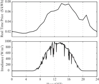
![Fig. 1.6 Variation in average installed cost based on PV system size, from [9]](https://thumb-us.123doks.com/thumbv2/123dok_us/762515.2596471/18.918.165.807.108.390/fig-variation-average-installed-cost-based-pv-size.webp)
![Fig. 1.13 Classification of microinverters with high-frequency transformers [24]: microinverter with (a) dc link, (b) pseudo dc link, and (c) no dc link](https://thumb-us.123doks.com/thumbv2/123dok_us/762515.2596471/25.918.197.779.102.360/fig-classification-microinverters-high-frequency-transformers-microinverter-pseudo.webp)
![Fig. 3.2 Common grid-tied PV system interconnection as shown in [41]](https://thumb-us.123doks.com/thumbv2/123dok_us/762515.2596471/59.918.253.715.803.1020/fig-common-grid-tied-pv-interconnection-shown.webp)