A Refactoring Technique for Large Groups of Software Clones Asif S. AlWaqfi A Thesis in The Department of
Computer Science and Software Engineering
Presented in Partial Fulfilment of the Requirements for the Degree of Master of Computer Science at
Concordia University Montréal, Québec, Canada
CONCORDIA UNIVERSITY Division of Graduate Studies This is to certify that the thesis prepared
By : Asif S. AlWaqfi
Entitled : A Refactoring Technique for Large Groups of Software Clones
and submitted in partial fulfilment of the requirements for the degree of
Master of Computer Science
complies with the regulations of this University and meets the accepted standards with respect to originality and quality.
Signed by the final examining committee :
Chair Dr. Tristan Glatard Examiner Dr. Weiyi Shang Examiner Dr. Emad Shihab Supervisor Dr. Nikolaos Tsantalis Approved by Dr. Volker Haarslev
Graduate Program Director 2017.
Dr. Amir Asif Dean of Faculty
ABSTRACT
Code duplication, also known as software clones, is a persistent problem in soft-ware systems that is usually associated with error-proneness and poor softsoft-ware main-tainability. Despite the fact that clone detection is a mature research field, clone refactoring has not been equally investigated. Clone refactoring requires the unifica-tion and merging of duplicated code, which is a challenging problem because of the changes that take place on the initial clones after their introduction.
In recent years, more research works attempted to address the challenges around clone refactoring by applying different techniques; however, they suffer from poor accuracy or performance issues, especially for large clone groups containing more than two clone instances. We contribute to this field by proposing an automated approach that a) finds refactorable subgroups (consisting of three clones or more) within the original group of clones, b) finds the statements that to be merged and extracted in a fast yet accurate way, and c) assesses the refactorability of clone subgroups.
We evaluated our approach in comparison to the state-of-the-art, and the results show that we have a high accuracy in matching the clone statements, while maintain-ing high performance. In a case study, where we carefully examined all clone groups in project JFreeChart 1.0.10, we found that around 49% of the 98 clone subgroups are actually refactorable. Finally, we conducted a large-scale study on over 44k clone groups (13.6k groups containing 3 clones or more) detected by four clone detection tools in nine open source projects to assess the refactorability for clone groups. The outcome of this study revealed the presence of 2,833 refactorable clone subgroups that contain in total 13,398 clone instances.
Acknowledgments
First and foremost, I would like to express my sincere gratitude to my advisor Dr. Nikolaos Tsantalis, for seeing my abilities and accepting me as one of his students. I would like to thank him also for his continues support towards my research and in writing my thesis, as well as for his patience and motivation which inspired and made me thrive to accomplish more in my research.
Apart from my advisor, I would like to thank my thesis examiners, Dr. Weiyi Shang and Dr. Emad Shihab, for taking the time to read my thesis and for their valuable suggestions and comments. I would like to thank other faculty members of the Department of Computer Science and Software Engineering as well, for the necessary guidance.
I thank my fellow lab mates and my friends in Concordia University for all their support towards the completion of this thesis. I express my gratitude to the staff members of our university for their help in providing a clean and safe environment for me to work.
Finally, I must express my very profound gratitude to my family for providing me with unfailing support and continuous encouragement throughout my years of study and through the process of researching and writing this thesis. This accomplishment would not have been possible without them.
Contents
List of Figures viii
List of Tables x
Table of Algorithms xii
1 Introduction 1
1.1 Motivation . . . 3
1.1.1 Duplicated Code is an extensive and persistent problem . . . . 3
1.1.2 Lack of reliable and mature clone refactoring tools . . . 6
1.1.3 Developers care about clones . . . 7
1.2 Contribution . . . 7
2 Background 9 2.1 Software Maintenance . . . 9
2.2 Code Clone Types . . . 10
2.2.1 Type I . . . 10
2.2.2 Type II . . . 11
2.2.3 Type III . . . 11
2.2.4 Type IV . . . 12
2.3.1 Clone Detection Techniques . . . 12
2.3.2 Challenges imposed by clone detection tools . . . 14
2.4 Algorithms . . . 15 2.4.1 String Similarity . . . 15 2.4.2 Vector Similarity . . . 16 2.4.3 Jaccard Index . . . 17 2.5 Clustering . . . 18 2.5.1 Hierarchical Clustering . . . 18 2.5.2 Silhouette Coefficient . . . 21
2.6 Program Dependence Graph . . . 22
2.7 Abstract Syntax Tree . . . 24
2.7.1 AST representation . . . 24
2.7.2 AST Visitor . . . 25
2.8 Clone Refactoring Preconditions . . . 25
3 Literature Review 29 3.1 Statement Mapping . . . 29
3.2 Clone Refactoring . . . 35
3.3 Program Dependence Graph Mapping . . . 39
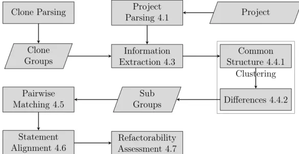
4 Approach 46 4.1 Project Parsing . . . 47
4.2 Clone Parsing . . . 48
4.3 Information Extraction . . . 48
4.3.1 Metric Approach . . . 49
4.3.2 Data Type Approach . . . 53 4.3.3 Additional information extracted commonly from all statements 55
4.4 Clustering . . . 55
4.4.1 Common Control Structure . . . 56
4.4.2 Differences . . . 59
4.5 Pairwise Matching . . . 62
4.5.1 Generating Similarity Matrices . . . 62
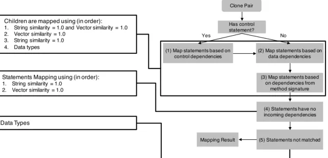
4.5.2 Statement mapping algorithms . . . 65
4.6 Statement Alignment . . . 70 4.7 Refactorability Assessment . . . 71 5 Qualitative Study 73 5.1 Results . . . 74 5.2 Discussion . . . 75 5.2.1 Accuracy Evaluation . . . 76 5.2.2 Performance Evaluation . . . 80 5.2.3 Clustering Evaluation . . . 87
5.2.4 Clone Group level Evaluation . . . 93
6 Empirical Study 97 6.1 Experiment Setup . . . 97
6.1.1 Projects . . . 97
6.1.2 Clone Detection Tools . . . 98
6.1.3 Experiment Machine . . . 100
6.2 Results and Discussion . . . 100
6.2.1 Statement Mapping Comparison . . . 101
6.2.2 Clone Group Refactorability . . . 107
6.2.3 Threats to Validity . . . 108
List of Figures
2.1 An example of Clone Type I . . . 11
2.2 An example of Clone Type II . . . 11
2.3 Example of Gapped Statements highlighted in red . . . 12
2.4 Example of poor quality clone fragments . . . 15
2.5 Example of Hierarchical Clustering (Dendrogram) . . . 19
2.6 Program Dependency Graph (PDG) . . . 23
2.7 Example of an AST . . . 24
2.8 Change in execution behavior (Figure 5. in Tsantalis et al. [TMK15]) 26 3.1 Clone group containing unique clones . . . 31
3.2 Example demonstrating the limitation of MCIDiff to match reordered statements. . . 32
3.3 Example showing a non-optimal and an optimal mapping for two clone fragments taken from Tsantalis et al. [TMK15] . . . 34
3.4 Example of systematic edit (Figure 1, Page 2 Meng et al. [Men+15]) . 37 3.5 An Example of Form Template Method refactoring taken from Hotta et al. [HHK12] . . . 40
3.6 An Example of Intertwined Clones taken from Komondoor et al. [KH01] 42 3.7 Quantitative data in IBM application, (Figure 9. Page 13 Komondoor et al. [KH01]) . . . 43
4.1 Workflow of the Approach . . . 47
4.2 Workflow of the Approach . . . 65
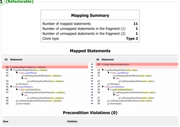
4.3 Example of a refactorable clone pair . . . 72
4.4 Example of a non-refactorable clone pair . . . 72
5.1 Example of different mapping . . . 77
5.2 Example of a statement mapping with more mapped statements . . . 79
5.3 Example of a statement mapping with less mapped statements . . . . 80
5.4 Execution time distribution: Our approach vs. Tsantalis et al. in millisecond . . . 83
5.5 Execution time distribution for each clone type in (ms) . . . 86
5.6 Change in a cluster after performing clustering based on Differences. . 88
5.7 The effect on clone types after performing clustering based on Differences. 89 5.8 The effect on clone types after performing clustering based on Differences. 90 5.9 The number of differences is reduced after performing clustering based on Differences, but the clone type remains the same. . . 91
5.10 The effect on the number of mapped statements after performing clus-tering based on Differences. . . 92
5.11 Example of a refactorable cluster with three clone instances. . . 94
5.12 Execution time for groups containing between 2-5 clones (Group-1) . 96 5.13 Execution time for groups containing between 6-12 clones (Group-2) . 96 6.1 Examined Projects [Tsab] . . . 98
List of Tables
1.1 Number of clone instances detected by each tool . . . 5
1.2 Percentage of groups containing 3 or more clone instances . . . 5
1.3 Percentage of groups containing x clone instances (3 ≤x ≤ 9) in the dataset [TMK15] . . . 5
4.1 AST Features in metric approach . . . 50
4.2 Results of metric approach at pair level . . . 51
4.3 Excluded types . . . 55
4.4 Info1 Elements . . . 59
4.5 Info2 Elements . . . 60
4.6 Features of the Feature Vector . . . 63
4.7 Statement Type . . . 63
5.1 Examined clone dataset . . . 74
5.2 Overall results . . . 74
5.3 Results included in the comparison . . . 75
5.4 Cases with non-identical statement mapping . . . 76
5.5 Execution time for each clone type . . . 84
5.6 The effect of clustering based on Differences on the initial clusters obtained by clustering based onCommon Structure . . . 87
5.7 Cluster refactorability results . . . 94
5.8 Groups based on Group Size . . . 95
6.1 Machine Specifications . . . 100
6.2 Percentage of groups containing more than 2 clone instances. . . 101
6.3 Total Clone Pairs being compared . . . 102
6.4 Number of Type I clones pairs per project . . . 103
6.5 Pairwise Statement Mapping comparison for Clone Type I . . . 103
6.6 Median Execution time for Pairwise Statement Mapping for Clone Type I . . . 103
6.7 Number of Type II clones pairs per project . . . 104
6.8 Pairwise Statement Mapping comparison for Clone Type II . . . 105
6.9 Median Execution time for Pairwise Statement Mapping for Clone Type II . . . 105
6.10 Number of Type III clones pairs per project . . . 106
6.11 Pairwise Statement Mapping comparison for Clone Type III . . . 107
6.12 Median Execution time for Pairwise Statement Mapping for Clone Type III . . . 107
List of Algorithms
1 Divisive clustering algorithm . . . 19
2 Agglomerative clustering algorithm . . . 20
3 Clustering using Common Control Structure . . . 58
4 Distance Matrix . . . 60
5 Clustering using Differences . . . 61
6 Vector Similarity Heuristic . . . 64
7 Initial Step in Pair matching . . . 66
8 Pair matching using Control Dependencies . . . 68
9 Pair matching based on Data Dependencies . . . 68
10 Pair matching for statements having no incoming dependencies . . . . 69
11 Matching of previously unmatched statements . . . 70
Chapter 1
Introduction
System development life cycle (SDLC) represents the phases a software has to go through until the user is able to interact with a running system. SDLC starts by col-lecting requirements from users (Analysis phase), designing the system as a collection of modules or subsystems (Design phase), implementing the design into source code (Implementation phase), and ends by testing and delivering the software product to the user (Testing phase). However, after the initial delivery of the product, the Maintenance phase starts, during which bugs are getting fixed or new requirements are being implemented.
Studies have shown that the Maintenance phase holds the largest percentage of the total software development cost. Grubb et al. [GT03] estimated that 40%-70% of the money spent on a system during its lifetime is spent on maintenance. Mobley [Mob90] and Maggard et al. [MR92] reported that 15%-40% of production cost is spent on maintenance. A study by Wireman [Wir89] estimated the maintenance cost for a group of companies would increase from $200 billions in 1979 to $600 billions in 1989. Coleman et al. [Col+94] reported that, in 1992, 60%-80% of the research and development staff at Hewlett-Packard were involved in maintenance tasks, and that
40%-50% of production cost was spent on maintenance.
The quality of code written during the Implementation phase affects significantly the effort require to complete future maintenance tasks. Dekleva [Dek92] reported in a survey that one of the most severe problems in maintenance is the quality of source code, while Chapin [Cha99] mentioned in a survey that 48% of maintenance problems are related to source code quality, such as poor documentation, high complexity, and poor code structure quality.
The improvement of source code quality can be achieved through restructuring.
Restructuring is defined by Chikofsky et al. [CC90] as "the transformation from one representation form to another at the same relative abstraction level, while preserving
the subject system’s external behavior (functionality and semantics)". A special case
ofrestructuring in object-oriented software development is Refactoring, a term
intro-duced by Opdyke [Opd92]. The object-oriented programming paradigm is based on the concept of “objects”, which may contain data, in the form of fields, often known as attributes; and code, in the form of procedures, often known as methods.
Refactoring improves the quality of software by removing code smells found in the code. Code smells according to Mens et al. [MT04] and Fowler et al. [Fow+99], are
"structures in the code that suggest (sometimes scream for) the possibility of
refac-toring" . There is a large variety of code smells, such as duplicated code (or referred
to as code clones), and Feature Envy (i.e., when a method uses more features from another class than the one it exists in). The focus of this thesis will be on duplicated code refactoring as a means to enhance software quality and maintainability.
Duplicated code (code clones) increase maintenance effort and cost [LW08], error-proneness when clones are updated inconsistently [Jue+09], and code instability [MRS12]. To address these problems, different techniques were proposed as part of clone management [Kos08]. Clone management [Kos08] can be preventive (i.e.,
avoid the introduction of new clones), corrective (i.e., eliminate existing clones), and
compensative (i.e., limit the negative impact of clones through automatic clone
syn-chronization when a change occurs). This work focuses on the corrective aspect of clone management. It proposes a new approach to handle clone groups containing three or more clone instances, by finding the differences among their statements, map-ping properly reordered statements, and finally assessing if the clones in the group can be safely refactored.
1.1
Motivation
The motivation behind this thesis comes from the three main points discussed exten-sively in the next sub-sections.
1.1.1
Duplicated Code is an extensive and persistent problem
Code clones can comprise a high percentage of systems code base. For instance, Wang and Godfrey estimated 10%-20% of the code in large systems are clones (a copy of other code with or without changes) [WG14], while Ducasse et al. reported the duplicated code in COBOL (COmmon Business Oriented Language, a programming language used to solve business problems [Mic]) systems was about 50% [DRD99] of the written code. Baxter et al. [Bax+98] detected that 12% of the code being duplicated; Baker [Bak95] identified 13%-20% of the code being cloned; Lague et al. [Lag+97] found that clone code is between 6.4%-7.5%; Mayrand et al. [MLM96] estimated the duplicated code in industrial systems ranges within 5% – 20%; and Ducasse et al. [DRD99] reported that clones can comprise 10% –15% of the source code of large systems. A survey done by Arcoverde et al. [AGF11] reported that the most persistent code smell is duplicated code.
To add further evidence, we used a publicly available clone dataset [TMK15] that includes the clones detected by four clone detection tools in 9 open source projects. According to Bellon et al. [Bel+07], the clone detectors that we selected have a precision (P) and recall (R) of: CCFinder (P: 72%, R: 72%), CloneDR (P: 100%, R:9%). Deckard is more scalable than CloneDR [Jia+07], and NiCad has a precision and recall of (P: 96%, R: 100%) [RC09]. For NiCad we used two configurations: Blind, all identifiers are replaced with a single pseudo-variable; while Consistent, the same identifier is replaced with a single pseudo-variable Xindex . The number of detected
clone instances are shown inTable 1.1. The numbers in the table represent number
of clones detected by each tool, where the last row is the total of clones detected by the tool in all examined projects. These clones are detected in groups, where the minimum size for each group is two (i.e., it contains only 2 clone instances). In the context of this thesis, we focus more on clone groups containing more than two instances, before the majority of previous works has mostly focused on clone pairs (i.e., groups of two clone instances).
Table 1.2 shows the percentage of clone groups containing more than two
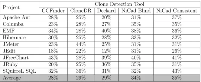
in-stances for each examined project. The last row represents the average percentage of groups that consist of three or more clone instances. The average percentage ranges between 28%-35% , showing that there is a significant number of clone groups with multiple instances (i.e., more than two instances). Moreover, these groups contain over 60% of the detected clone instances with a total of 94,650 instances. Table 1.3 shows the percentage of groups detected by each clone detection tool, where groups are categorized based on the number of clone instances they contain. The groups containing 3, 4, and more than 9 clone instances have the highest percentage, while the other categories range from 0.6% to 2.67%.
Table 1.1: Number of clone instances detected by each tool
Project CCFinder CloneDR Deckard NiCad Blind NiCad ConsistentClone Detection Tool
Apache Ant 2,798 4,071 1,812 2,853 2,282 Columba 2,046 3,987 1,925 2,260 1,627 EMF 5,479 5,973 955 4,690 3,851 Hibernate 3,733 6,191 3,581 3,041 2,314 JMeter 2,018 525 1,974 2,187 1,703 JEdit 939 1,630 864 1,209 863 JFreeChart 9,546 8,804 6,932 4,793 4,211 JRuby 3,257 4,212 1,628 3,293 2,373 SQuirreL SQL 7,299 8,646 2,204 4,765 3,800 Total 37,115 44,039 21,873 29,091 23,024
Table 1.2: Percentage of groups containing 3 or more clone instances
Project CCFinder CloneDR Deckard NiCad Blind NiCad ConsistentClone Detection Tool
Apache Ant 28% 25% 20% 31% 37% Columba 23% 28% 27% 35% 35% EMF 34% 28% 40% 38% 36% Hibernate 30% 25% 28% 33% 32% JMeter 23% 44% 25% 31% 31% JEdit 18% 22% 12% 31% 26% JFreeChart 43% 28% 39% 40% 41% JRuby 20% 25% 36% 35% 31% SQuirreL SQL 32% 36% 31% 32% 43% Average 28% 29% 29% 34% 35%
Table 1.3: Percentage of groups containing x clone instances (3 ≤ x ≤ 9) in the
dataset [TMK15]
Tool / Group Size 3 4 5 6 7 8 9 > 9
CCFinder 11.42% 7.69% 2.70% 2.23% 1.10% 1.04% 0.75% 3.47% CloneDR 12.43% 5.95% 2.43% 1.95% 1.07% 0.88% 0.51% 3.24% Deckard 15.49% 6.99% 2.08% 1.80% 0.85% 0.84% 0.40% 1.94% NiCad Blind 15.22% 7.91% 3.09% 2.52% 1.11% 1.17% 0.68% 4.55% NiCad Consistent 14.84% 7.77% 3.05% 2.65% 1.19% 1.23% 0.71% 4.26% Average 13.88% 7.26% 2.67% 2.23% 1.06% 1.03% 0.61% 3.49%
1.1.2
Lack of reliable and mature clone refactoring tools
As mentioned before, clone management encompasses three categories of actions; however, researchers in the field mainly focused on two of them, namely preven-tive and compensapreven-tive. Many tools and techniques were developed and proposed by researchers such as, CCFinder [KKI02], and NICAD [RC08b] to assist developers in finding clones scattered through project files. Other tools such as CloneTracker [DR08; Ngu+12] act as live recommendation systems to notify users of clones being modified.
The corrective aspect of clone management covers the elimination of clones through refactoring. The process of refactoring requires first to compare the code clones and find differences between them, such as different method calls that need to be pa-rameterized in the common code that will be extracted (i.e., a parameter should be introduced in the extracted common code for each difference found in the clones).
Current clone refactoring tools support mostly trivial differences for parameteri-zation. Eclipse allows only differences in local variable names, and it can be applied on clones within the same Java file only. CeDAR is another Eclipse plug-in pro-posed and developed by Tairas et al. [TG12], which extends the Eclipse refactoring engine to allow more kinds of differences between the clones. CeDAR was able to refactor 18% of the cases reported by Deckard in comparison to 10.6% that could be refactored by Eclipse. However, CeDAR is limited to Type-1 (i.e., same code except
for differences in whitespace or comments) andType-2 (i.e., clones containing
differ-ences in identifiers, literals, and types) clones. Meng et al. [Men+15] is the first work that supports more advanced clone refactoring operations, by extracting the common code, creating new types and methods (if necessary), and introducing return objects, but despite these improvementsType-3 (i.e., clones with statements added, removed,
or changed) clones are not supported.
Lastly, a work done by Tsantalis et al. [TMK15] can be seen as the state-of-the-art tool in refactoring pairs of clones (i.e., groups containing two clone instances) that addressed all previous limitations and supports automated refactoring. The only limitation is that it does not support the refactoring of clone groups containing more than two clone instances.
1.1.3
Developers care about clones
In a survey conducted by Yamashita et al. [YM13], about determining the knowledge of developers and their interest in code smell, one of the questions asked to developers was to rank code smells according to their perceived importance"Are there specific code smells / anti-patterns that you are concerned about? Please list them in order of their perceived importance". Duplicated Code was the most popular
smell and had thehighestrank with 19.53 points (Table 4, Yamashita et al. [YM13])
followed by Long Method with 9.78 points, Accidental Complexity with 8.32 points, and Large Class with 7.09 points.
In another survey by Silva et al. [STV16] it was observed that developers are seriously concerned about avoiding code duplication, when working on a given main-tenance task. Developers often apply refactorings, especially Extract Method refac-torings, to reuse code and avoid duplicating the same functionality.
1.2
Contribution
This work deals with the problem of refactoring (or merging) clone groups containing three or more clone instances. The main challenge is the scalability of the solution, since as the size of a clone group increases, the number of pair-wise clone instance
comparisons/combinations grows factorially n 2
. The contribution of this work can be summarized as:
1. We propose a multi-clone statement mapping approach that uses control and
data dependence information as well as date type information.
2. We propose an algorithm to find subgroups of clone instances that have a min-imum number of differences, within a group of clones. In this way, we reduce the number of combinations to be examined, because we avoid the comparison of clones in different subgroups.
3. We show evidence that large clone groups can become refactorable by splitting them into smaller subgroups.
The rest of the thesis is organized as follows: Chapter 2 covers background knowl-edge that is needed throughout the thesis. Chapter 3 contains a review of the related literature. Chapter 4 describes the proposed solution for multi-clone analysis and refactoring. Chapter 5 presents a qualitative study on 847 clone groups containing 2307 clone instances in total. Chapter 6 contains statistical information from the analysis of clone groups detected by 4 different clone detection tools in 9 open-source projects. Finally, the conclusions of the thesis and future work are discussed in Chapter 7.
Chapter 2
Background
2.1
Software Maintenance
Software Maintenance is the last phase and an important part of System Develop-ment Life Cycle (SDLC), because systems evolve and new requireDevelop-ments are needed as time passes. Lientz et al. [LS81] reported in a survey that around half of the devel-opment time is spent on maintenance, and over forty percent of the time is spent on enhancements and adding new features to running systems. Software Maintenance is classified into four types [Tsu+15] based on the goal it carries out:
• Adaptive: Ensure system compatibility with the changes in its environment.
For instance, sometimes there are improvements to the hardware the system is running on; however, the software needs to be updated to ensure the system will keep running normally and will not fail.
• Perfective: Improve the performance and maintainability of a working system.
• Corrective: Identify and correct problems in a system, after it has been pushed
• Preventive: Prevent potential faults occurring in the future. The system is
still running perfectly with no bugs, but the developers realize that they have to do some changes to prevent faults in the future if certain conditions are met. Our work in this thesis is associated with the following maintenance types:
Perfective because duplicated code degrades the quality of the system, which affects
future maintenance tasks.
Corrective because duplicated code increases the effort required to fix existing bugs
repeated in many different places of the source code.
Preventive because maintenance is a continuous process and duplicated code can
be a source of inconsistent changes and future bugs.
2.2
Code Clone Types
Copying existing functionality to create new one by making minor modifications can lead to divergent clones (i.e., pieces of code that were originally the same, but
become syntactically more distant after they undergone some modifications ). Some of these changes may include renaming variables, removing or adding statements, changing method calls or instantiated objects. Based on the changes duplicate code is categorized into four types [RCK09].
2.2.1
Type I
The duplicated code, excluding differences in white-spaces, comments, and layout is exactly the same.
Figure 2.1: An example of Clone Type I
2.2.2
Type II
Type IIis a superset of Type I, additionally including differences in the identifiers,
literals, and types.
Figure 2.2: An example of Clone Type II
2.2.3
Type III
Type III is a superset of Type II with further modifications such as, added,
re-moved, or changed statements. Statements that appear in one clone fragment, but not the others are called gapped/unmapped statements. Figure 2.3 below is an exam-ple of a pair of matched clones were statements 21-22 are considered as gaps, because they appear in the left fragment only and could not be mapped with any statement in the second fragment on the right.
Figure 2.3: Example of Gapped Statements highlighted in red
2.2.4
Type IV
This type is very difficult to be detected by clone detection tools, due to clones having a completely different syntactic implementation, but similar functionality [RCK09; RC09]. Also, it is not necessary that they were copies of each other, as they might be coded by different developers [RC07]. Below is an example of a Type-4 clone were one of the fragments is written using a while-loop, while the other uses a recursive-function:
void l o o p O v e r (int var ) {
wh ile( var > 0) {
S y s t e m . out . p r i n t l n ( var ) ; var - -;
} }
void l o o p O v e r (int var ) {
if( var > 0) {
S y s t e m . out . p r i n t l n ( var ) ; l o o p O v e r ( - - var ) ;
} }
2.3
Clone Detection tools
2.3.1
Clone Detection Techniques
There are many available tools for detecting clones in source code. These tools use different techniques to detect duplicate code [RCK09], for which we will give a general overview in this section along with some indicative tools.
2.3.1.1 Textual technique
In this approach the raw source code is textually compared after some normalization and formatting of the source code before the comparison is executed.
- Tools following this approach are NiCad [RC08a] and Simian [Har16].
2.3.1.2 Lexical technique
This technique is referred to as token-based approach. The source code is converted into a sequence of tokens, which are scanned for duplicate sub-sequences.
- Tools following this approach are CCFinder [KKI02] and CP-Miner [Li+06].
2.3.1.3 Syntactic technique
In contrast to previous techniques, this technique requires the source code to be parsed into an abstract syntax tree (AST), and then either a tree or structural matching
approach is used to detect clones.
• Tree matching approach detects clones by finding similar sub-trees.
- Tools following this approach are CloneDR [Bax+98] and ccdiml [Pro].
• Metrics-Based approach Metrics from code fragments are gathered in feature
vectors, and then the similarity of these feature vectors is computed.
- Tools following this approach are DECKARD [Jia+07] and SMC-Similar Method Classifier [Bal+99].
2.3.1.4 Semantic technique
This technique uses static analysis to generate the Program Dependence Graph (PDG) of functions, and then finds isomorphic sub-graphs.
- A tool following this approach is the tool developed by Jens Krinke [Kri01]
There are many techniques and tools to detect clones; however, their performance and results impose other challenges that need to be addressed before they can be used for the purpose of clone refactoring.
2.3.2
Challenges imposed by clone detection tools
Quality of clones Figure 2.4 shows an example of poor quality clone fragments
reported by NiCad in JFreechart project, where only two statements have been mapped while the other statements couldn’t be mapped because their abstract syntax tree structure is different. Moreover, some of the groups reported by clone detection tools can be very large, such as 200 clone instances or more in the same group, which puts in question the quality of such a clone group. Finally, the number of statements inside the clone fragments can be problematic, as some tools might report a single statement as a clone.
Incomplete control structure Clone detection tools do not preserve the control
structure and report clones with partial control structure. For instance, if the original source code contains If-Else, the clone detection tool might return only the if clause, or the else clause. So, we refer to control statements that all of their nested statements are included in the reported clone fragments as Complete Control statements.
Non-Refactorable clones Some clones do not have the aforementioned limitations,
but they cannot be refactored, because the fragments belong to different files and the extracted code cannot be pulled up into a common superclass.
Figure 2.4: Example of poor quality clone fragments
2.4
Algorithms
2.4.1
String Similarity
2.4.1.1 Levenshtein Distance
This algorithm was named after Vladimir Levenshtein [Lev66]. Levenshtein Distance (LD) is one of the widely known and used algorithms to measure the similarity be-tween two strings. The distance is measured by computing the minimum number of deletions, insertions, or substitutions required to transform one string into another. The LD distance for two strings A and B is computed as:
LD(A, B) = min{a(i) +b(i) +c(i)} (2.1)
where a(i), b(i), and c(i) are number of replacement, insertion, and deletion
op-erations, respectively. To compute the similarity between strings A, and B we use
equation 2.2.
similarity(A, B) = 1− LD(A, B)
2.4.2
Vector Similarity
Before we discuss vector similarity algorithms we need to mention that each vector in the computation should have the:
• Same Dimension
• Same Length
• Same Features being compared. Feature X in one vector should be compared
to the same feature in the other vector.
2.4.2.1 Cosine Similarity
Cosine Similarity is one of the popular algorithms in text mining and information retrieval [Deh+11], where the similarity between two vectors A and B is computed
as: similarity(A, B) = Pl i=1(Ai.Bi) (Pl i=1(Ai)2).( Pl i=1(Bi)2) (2.3) wherel is the length of vector, Ai andBi correspond to the same feature iin vectors
A and B. Because the formula of this algorithm is a dot product, ifAi =Bi = 0 the
similarity will be 0 rather than 1.
2.4.2.2 Hamming Distance
This distance is used often to find the differences in two strings of bits equal in length. The earliest use for it was in 1980, when it was used to measure errors in messages sent over the network [BKR02]. The advantage of using this algorithm is that when two vectors have the same feature equal to 0, it means that the similarity for this feature is 1 rather than 0 as in Cosine similarity. For two feature vectors A and B
distance(A, B) = l X i=1 0 if Ai=Bi 1 if Ai6=Bi (2.4) wherelis the dimension of the vectors. While the similarity forAandB is computed
as:
similarity= 1−distance(A, B)
|vector| (2.5)
where |vector| is the length of A and B. Equation (2.4) and (2.5) can be re-written
as: similarity(A, B) = Pl i=1 1 if Ai=Bi 0 if Ai6=Bi |vector| (2.6) 2.4.2.3 Euclidean distance
This metric is the distance or line that connects two points A and B in n-space.
Euclidean distance has been used in different fields such as, clustering [PJ09].
distance(A, B) = v u u t n X i=1 (Ai−Bi)2 (2.7)
2.4.3
Jaccard Index
In 1901 Paul Jaccard introduced Jaccard Index or what is known as Jaccard similarity coefficient [BJD13]. It is used to measure the similarity between two sets. Assuming
A and B are sets, then Jaccard similarity is computed as:
similarity(A, B) = |A∩B|
|A∪B| (2.8)
2.5
Clustering
Clustering is an analysis done to data in a group with the goal to divide them into smaller groups by putting together the similar data points (Equation 2.9) [RM05]. We will discuss one of the commonly used clustering algorithms, namely Hierarchical Clustering. S= n [ i=1 Ciand Ci∩Cj =∅f or i 6=j (2.9)
where clusters C1...Cn are subsets of S.
2.5.1
Hierarchical Clustering
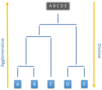
In this type of clustering you don’t need to specify or know the number of clusters beforehand, in contrast to other algorithms, such as K-means, in which the number of clusters should be given as input. However, you need to know what level of clustering is the best. There are algorithms such as the Silhouette Coefficient [Rou87] that can help to estimate what level of clustering is the best, which we will discuss later on. There are two approaches in hierarchical clustering based on the starting point as they appear in Figure 2.5, namely Divisive and Agglomerative.
A B C D E Ag gl om er at iv e Di vis ive A B C D E
Figure 2.5: Example of Hierarchical Clustering (Dendrogram)
2.5.1.1 Approaches
Divisive (Top - Down) This approach starts by placing all data points in the same
cluster(Top), and then it starts splitting the clusters into smaller clusters until each
data point is placed in a separate cluster (Down). The partitioning function can
be based on for example, the size of the cluster (split largest clusters first), and the average similarity between clusters [DH02]. Algorithm 1 presents the procedure to cluster M points in a divisive manner.
Algorithm 1: Divisive clustering algorithm Input: M points
Output: Dendrogram
1 clusters← ∅
2 clusters←clusters∪M points 3 while |clusters| 6=|M| do
Agglomerative (Bottom - Up) This approach starts by putting each data point
in its own cluster(Bottom), then merge the data points one pair at a time based on
their similarity (or distance) until there is a single cluster that contains all data points
(Up). Algorithm 2 presents the procedure to cluster M points in an agglomerative
manner.
Algorithm 2: Agglomerative clustering algorithm Input: M points
Output: Dendrogram
1 clusters← ∅
2 clusters←clusters∪M clusters forM points 3 while |clusters|>1 do
4 merge nearest clusters in clusters
2.5.1.2 How to merge two clusters?
There are different algorithms to combine clusters [ZKF05], and some of them are mentioned below. Assuming pk is a point in cluster Ci, pr is a point in cluster Cj,
and similarity is the function used to compute the similarity or distance between
two points:
Single Linkage The similarity for(Ci, Cj)is the highest similarity between pairwise
points in Ci and Cj. After applying equation 2.10 on all pairs of clusters, the
clusters with the maximum similarity are merged.
simsingle(Ci, Cj) =maxpk∈Ci,pr∈Cj(similarity(pk, pr)) (2.10)
Complete Linkage This approach is the opposite of Single-Linkage, as the
simi-larity between two clusters is the lowest simisimi-larity (highest distance) between their pairwise points. After applying equation 2.11 on all pairs of clusters, the
clusters with minimum similarity (maximum distance) are merged together.
simcomplete(Ci, Cj) =minpk∈Ci,pr∈Cj(similarity(pk, pr)) (2.11)
Average Linkage This clustering is referred to as UPGMA scheme [JD88]. The
similarity between two clusters is computed by finding the average similarity between all points in the two clusters.
simaverage(Ci, Cj) = ( 1 |Ci||Cj| ) X pk∈Ci,pr∈Cj similarity(pk, pr) (2.12)
MinMax Linkage This algorithm was proposed by [Din+01]. The goal is to merge
clusters that are less self-similar.
simM inM ax(Cp, Cq) =
sim(Cp, Cq)
sim(Cp, Cp)sim(Cq, Cq) (2.13)
2.5.2
Silhouette Coefficient
Silhouette Coefficient was introduced by Rousseeuw [Rou87]. It is used to measure and estimate the consistency and quality of clusters.
SilhouetteScore= Pn i=1 P|Ci| j=1s(j) |m| (2.14) s(j) = bX[j]−aX[j] max(bX[j], aX[j]),(−1≤s(j)≤1) (2.15) where
Ci is the cluster at iteration i, and |Ci| the cardinality of it
bX is the average dissimilarity between point j in cluster Ci and points outsideCi
aX is the average dissimilarity between point j in cluster Ci and its points
m is the total number of points in all clusters, and |m| the cardinality of it
The closer s(j) to 1 the less the dissimilarity within the same cluster and greater
to the other clusters (aX < bX), so we can say j is well-clustered. However, when j ismisclassified the dissimilarity within the same cluster is greater than the other
clusters, and s(j) will be close to -1 (aX > bX). In the situation where aX ≈ bX,
the value of s(j) will be close to 0, which implies it is not clear if j is placed in the
appropriate cluster or not.
2.6
Program Dependence Graph
The Program Dependence Graph (PDG) represents the relation between program elements, where elements are statements or predicates. The edges represent rela-tions that connect these elements, which can be either data or control dependencies [FOW84]. Data dependencies are further categorized into three types [WB87]. As-sumingS1 and S2 are statements, then:
1. Data-Flow Dependency S1 R
−→
d S2: Assuming that S2 uses a result R from
executingS1, then we say that S2 is data dependent on S1.
2. Output Dependency S1 R
−→o S2: Assuming R is the result from executingS1.
IfS2 modifies R then we say S2 is output dependent on S1.
3. Anti DependencyS1 R
−→a S2: AssumingRis a variable used inS1 and modified
4. Control Dependency S1 T orF
−−−→
c S2: Assuming S1 is a control statement (If,
For,. . . ). If the execution ofS2 depends on the result of S1 then we say thatS2
is control dependent on S1. A control dependency is labeled as either True or
False. For example, the control dependencies to the statements inside the else
clause of an If/Else statement are labeled asFalse. All other control
dependen-cies are labeled as True.
1) int x = 2; 2) if (x > 0) { 3) int y = x; 4) int z = y + 1; 5) y = 10;; } 1 2 3 4 5 Control Dep Data Dep Anti Dep Output Dep T T T x x y y y
Figure 2.6: Program Dependency Graph (PDG)
In the figure above, x and y are the variables affected by each dependency, also T stands forTrue control dependency.
2.7
Abstract Syntax Tree
2.7.1
AST representation
The Abstract Syntax Tree (AST) represents the syntactic structure of the source code inside a file, which is derived from the parse tree or more often referred to as Concrete Syntax Tree (CST). CST contains all information about the source code, including comments, white-spaces, and line-breaks. The AST representation is an abstraction of the CST that keeps only the information necessary to the compiler. Figure 2.7 shows the AST representation for the code below. The content of Figure 2.7 is generated using the Eclipse plug-in AST-View [Foua].
p u b l i c cla ss s i m p l e A S T { p r i v a t e int x = 0; p u b l i c int getX () { r e t u r n x ; } } TypeDeclaration (class) NAME SimpleName simpleAST MODIFIERS(1) Modifier public BODY_DECLARATIONS(2) FIELDDECLARATION MethodDeclaration MODIFIERS(1) Modifier private TYPE PrimitiveType int FRAGMENTS(1) VariableDeclarati onFragment NAME MODIFIERS(1) Modifier public RETURN_TYPE2 PrimitiveType int NAME SimpleName getX SimpleName x BODY Block STATEMENTS(1) ReturnStatement Expression SimpleName x
2.7.2
AST Visitor
The ASTVisitor is an abstract class found in org.eclipse.jdt.core.dom [Foub] library
which is part of the Eclipse IDE. It provides a mechanism to explore or visit every statement and expression in an AST, and to perform an operation on specific types of AST nodes. A class is required to extend ASTVisitor and override the methods
visit, and endVisitto implement custom functionalities.
2.8
Clone Refactoring Preconditions
The goal of this section is to introduce the conditions that duplicate code at pair or group level must comply with to be assessed as refactorable. These conditions are proposed by Tsantalis et al. [TMK15] and we will use them in evaluating the refactorability of clone groups. There are eight preconditions in total, which we will discuss next.
Precondition 1
The parameterization of the differences between the mapped statements should not break any existing control, data, anti, and output dependencies.
In the example shown in Figure 2.8, the behavior of code has changed after apply-ing refactorapply-ing because it violated this precondition. In the original code (Before refactoring) in class B, a.getX() is assigned to variable x in methods m1 and m2,
then a.foo() and a.bar() are called. Both a.foo() and a.bar() change the value of
field x that exists in class A. To refactor m1 and m2 the common code needs to
be extracted to a new method and parameterize the differences in the statements. The differences are the calls for a.foo() and a.bar() in m1 and m2, respectively.
However, passing these method calls as arguments will first update field x of class
A, and then assign it to variable x in the extracted method, thus changing the final
result that is printed and the behavior of the program.
Before Refactoring After Refactoring
public class A {
private int x;
public int getX () { return x; }
public int foo () { x++; return x; }
public int bar () { x+=5; return x;}
}
public class B {
public void test () {
A a = new A();
m1(a); m2(a); }
public void m1(A a) {
int x = a. getX ();
int y = a. foo ();
System.out.print (x); }
public void m2(A a) {
int x = a. getX (); int y = a.bar (); System.out.print (x); } } public class A { private int x;
public int getX () { return x; }
public int foo () { x++; return x; }
public int bar () { x+=5; return x; }
}
public class B {
public void test () {
A a = new A();
m1(a); m2(a); }
public void m1(A a) {
ext (a, a. foo ()); }
public void m2(A a) {
ext (a, a. bar ()); }
private void ext (A a, int arg ) {
int x = a. getX ();
int y = arg ;
System.out.print (x); }
}
Figure 2.8: Change in execution behavior (Figure 5. in Tsantalis et al. [TMK15])
Precondition 2
Matched variables having different subclass types should call only methods that are declared in the common superclass or are being overridden in the respective subclasses.
Precondition 3
The parameterization of fields belonging to differences between the mapped state-ments is possible only if they are not modified.
In this precondition, fields that are part of the differences are only parameterizable if they are not modified in the extracted code. In other words if the field’s value
is changed inside the extracted code then this difference cannot be parameterized, because parameters are passed by value in Java, and thus the extracted code would not update the values of the fields after the refactoring.
Precondition 4
The parameterization of method calls belonging to differences between the mapped statements is possible only if they do not return a void type.
Precondition 5
The unmapped statements should be movable before or after the mapped statements without breaking existing control, data, anti, and output dependencies.
Precondition 6
The mapped statements within the clone fragments should return at most one vari-able of the same type to the original methods from which they are extracted. This condition implies that after extracting the mapped statements into a new method, the method should return at most one variable of the same type, since in our case the programming language is Java and it does not support passing of parameters by reference. On the contrary, languages supporting parameter passing by reference, such as C and C++, can return multiple variables.
Precondition 7
The mapped statements within the clone fragments should not contain any condi-tional return statements.
The following example shows a conditional return statement. These statements are used to exit directly the method they exist in. However, if we extract statements (1) and (2) to a new method, they will exit the execution of the extracted method,
while the original methodfoo() will continue to execute normally and will not exit.
This problem can be solved by returning boolean flag from the extracted method; however, this solution will require to add new statements to the original codefoo()
and to the extracted method.
public void foo(){ int x = 0; . . . (1) if (x > 0) (2) return ; System.out.println(x); . . . } Precondition 8
The mapped branching statements (break, continue) should be accompanied with the corresponding mapped loop statements.
This precondition implies that if the common statements include a break or con-tinue statement, then the corresponding loop (For, While, Do/While, Enhanced For) statement should be extracted as well.
Chapter 3
Literature Review
3.1
Statement Mapping
Lin et al. [Lin+14] work focused on how to find differences among multiple clones in the same group using Progressive alignment, an algorithm used in genetics to
align DNA and proteins [HS88]. They developed an Eclipse plugin called MCIDiff
(Multi-Clone-Instances Differencing) that takesN clones as an input and returns the
token differences among them. Their approach starts by parsing each clone into a sequence of tokens and each token is categorized into either Type, Method/Field/-Variable/Literal, Label, Keyword, or Separator (e.g., (,{), and Operator. The six
token classifications are divided into three groups based on the attributes attached to them: 1) Name: for Type, Method/Field/Variable/Literal and Label tokens; 2) Symbol: for Keyword, Separator and Operator tokens; lastly, 3) Data type: for Method/Field/Variable/Literal tokens.
After parsing is complete, in the first step, MCIDiff computes the Longest Com-mon Subsequence (LCS, longest sequence of tokens comCom-mon between all clones) using
and then proceeding with the next token sequence and so on. The resulting tokens in the LCS have the same category and attribute. However, there might be tokens that are not common in all sequences, thus they are returned as differential ranges representing the start and end indices for a range of tokens that were not common in all sequences.
Differential ranges are examined again to find common tokens within non-gapped tokens. First, they try to match identical tokens by re-running MCIDiff on non-gapped token sequences within the differential ranges and try to match them with the same criteria as before (same category and attribute). Then, for non-identical unmatched tokens a similarity heuristic is used (i.e., tokens should have the same cat-egory, while for attributes a similarity value is calculated). The computed similarity for Keyword/Separator/Operator/Label is equal to 1.0 if they are the same, other-wise it is 0.0; and for Type/Method/Field/Variable/Literal, the Jaccard coefficient [BJD13] is used to find if tokens have a super type in common.
To evaluate the accuracy of MCIDiff, they used 831 clone sets reported by CloneDe-tective (i.e., a token-based clone detection tool) [Jue+09] in three projects (Ja-vaNewIO, JHotDraw, JFreechart). They filtered the clone sets to keep only those that contain gaps and parameterization (i.e., differences), which resulted in only 638 (77%) clone sets, that consist of 353 sets containing two clones, 235 sets containing three-to-five clones, and 50 sets containing more than 5 clones. The (precision, recall) of MCIDiff for the three projects is respectively (100%, 100%), (98.66%, 95.63%), and (98.82%, 98.39%). While they have a good precision and recall, their work has several limitations that are listed below.
• Refactoring is not supported.
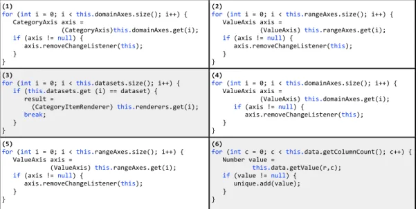
• They detect differences through Progressive alignment, but having a unique sequence might lead to incorrect alignment. For example, in Figure 3.1 we can
see that clones (1), (2), (4), (5) look similar in terms of control statements and the behavior or the operation they execute (i.e., removing an object from a list). However, clones (3) and (6) have different behaviors (unique clones) (i.e., clone (3) is searching for an object, and clone (6) is adding elements to a list).
(1)
for (int i = 0; i < this.domainAxes.size(); i++) { CategoryAxis axis =
(CategoryAxis)this.domainAxes.get(i);
if (axis != null) {
axis.removeChangeListener(this);
} }
(2)
for (int i = 0; i < this.rangeAxes.size(); i++) { ValueAxis axis =
(ValueAxis) this.rangeAxes.get(i);
if (axis != null) {
axis.removeChangeListener(this);
} } (3)
for (int i = 0; i < this.datasets.size(); i++) { if (this.datasets.get (i) == dataset) { result =
(CategoryItemRenderer) this.renderers.get(i);
break; } }
(4)
for (int i = 0; i < this.domainAxes.size(); i++) { ValueAxis axis =
(ValueAxis) this.domainAxes.get(i);
if (axis != null) {
axis.removeChangeListener(this);
} } (5)
for (int i = 0; i < this.rangeAxes.size(); i++) { ValueAxis axis =
(ValueAxis) this.rangeAxes.get(i);
if (axis != null) {
axis.removeChangeListener(this);
} }
(6)
for (int c = 0; c < this.data.getColumnCount(); c++) { Number value = this.data.getValue(r,c); if (value != null) { unique.add(value); } }
Figure 3.1: Clone group containing unique clones
• Finding similar tokens is almost an exhaustive search. As a result, the compu-tation time increases dramatically as the size of the clone group, the length of token sequences, and the number of differences among the clones increases.
• Examining the token sequences (i.e., clones) in a different order during the alignment process, might produce different results.
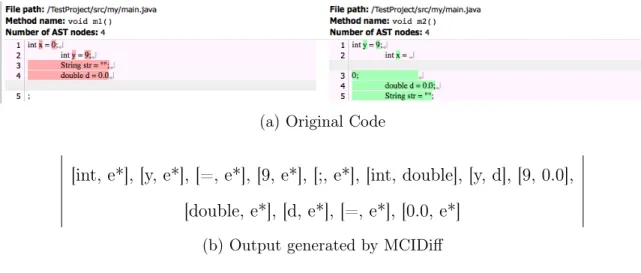
• Reordered statements are considered as gaps, because their approach treats the entire clone fragments as sequences of tokens. The example in Figure 3.2 demonstrates the limitation of MCIDiff. As it can be observed from the output of MCIDiff shown in Figure 3.2b the re-ordered statements String str = "";
(a) Original Code
[int, e*], [y, e*], [=, e*], [9, e*], [;, e*], [int, double], [y, d], [9, 0.0], [double, e*], [d, e*], [=, e*], [0.0, e*]
(b) Output generated by MCIDiff
Figure 3.2: Example demonstrating the limitation of MCIDiff to match reordered statements.
The results from MCIDiff 3.2b are interpreted as followa:
– Statements int y = 9;anddouble d = 0.0;in the first and second clone
fragments, respectively are considered as gaps.
– The pairs of tokens (int, double), (y,d), (9,0.0) are considered as
differ-ences between the two fragments.
A recent work by Tsantalis et al. [TMK15] assesses the refactorability of clone pairs by examining if the differences between the clones can be parameterized without causing any problems. Their approach consists of three major steps. The first step finds a common nesting structure (isomorphic trees) shared by the pair of clones. The second step maps the statements of the clones in a way that maximizes the number of mapped statements, while minimizes the number of differences between them. The last step examines a list of preconditions to check if the differences found between the clones can be safely parameterized, which we discussed in section 2.8.
structure trees (NST) of the clone fragments, and if there are more than one non-overlapping sub-trees, then each one is treated as a separate refactoring opportunity. They follow a combination of Bottom-Up and Top-Down matching approaches when searching for isomorphic sub-trees. They start from the leaf nodes and for each pair of matched leafs (Bottom-Up), they try to find a matching sibling. For each pair of matching siblings, they perform Top-Down matching to check if the resulting common sub-tree is complete (i.e., all child nodes in the sub-trees have been matched with one node from the other sub-tree). If a leaf in the first tree has multiple matches in the second tree, then only the first matching leaf with minimum differences is explored.
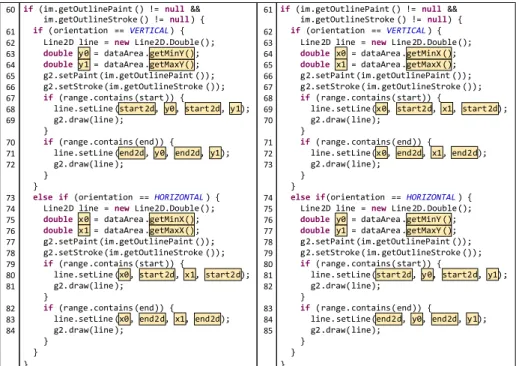
After finding the isomorphic trees (common structure) for a pair of fragments, the process of statement mapping follows. Each statement in the first fragment is mapped with a single statement at most in the second fragment. Figure 3.3 shows an example that the isomorphic trees resulting from the first step, do not lead to the best solution, as the number of differences in Figure 3.3a are 24, while if we switch the If/Else-If as in Figure 3.3b the number of differences decreases to only 2. This is solved by comparing the body of If in the first fragment with the bodies of If, and Else-If in the second fragment, and testing whether the resulting mapping maximizes
the number of mapped statements and at the same time minimizes the number of differences between the mapped statements. The second step of their approach is essentially a greedy algorithm that makes locally optimal choices at each level of the NST sub-trees with the hope of finding a globally optimal solution.
if wim.getOutlinePaint w}AM=Anull cc im.getOutlineStroke w}AM=Anull}A{
ifworientationA ==AVERTICAL}A{ Line2DAlineA=AnewLine2D.Doublew};
double y0A=AdataArea .getMinYw};
double y1A=AdataArea .getMaxYw}; g2.setPaint wim.getOutlinePaint w}}; g2.setStroke wim.getOutlineStroke w}}; if wrange.contains wstart}}A{ line.setLine wstart2d,Ay0,Astart2d,Ay1}; g2.drawwline }; } if wrange.contains wend}}A{ line.setLine wend2d,Ay0,Aend2d,Ay1}; g2.drawwline }; } }
else if worientationA ==AHORIZONTAL}A{ Line2DAlineA=AnewLine2D.Doublew};
double x0A=AdataArea .getMinXw};
double x1A=AdataArea .getMaxXw}; g2.setPaint wim.getOutlinePaint w}}; g2.setStroke wim.getOutlineStroke w}}; if wrange.contains wstart}}A{ line.setLine wx0,Astart2d,Ax1,Astart2d}; g2.drawwline }; } if wrange.contains wend}}A{ line.setLine wx0,Aend2d,Ax1,Aend2d}; g2.drawwline }; } } }
ifwim.getOutlinePaint w}AM=Anull cc im.getOutlineStroke w}AM=Anull}A{
ifworientationA ==AVERTICAL}A{ Line 2DAlineA=AnewLine 2D.Doublew};
double x0A=AdataArea .getMinX w};
double x1A=AdataArea .getMaxX w}; g2.setPaint wim.getOutlinePaint w}}; g2.setStroke wim.getOutlineStroke w}}; ifwrange.containswstart}}A{ line.setLinewx0,Astart2d,Ax1,Astart2d}; g2.drawwline}; } ifwrange.containswend}}A{ line.setLinewx0,Aend2d,Ax1,Aend2d}; g2.drawwline}; } }
else ifworientationA ==AHORIZONTAL}A{ Line 2DAlineA=AnewLine 2D.Doublew};
double y0A=AdataArea .getMinY w};
double y1A=AdataArea .getMaxY w}; g2.setPaint wim.getOutlinePaint w}}; g2.setStroke wim.getOutlineStroke w}}; ifwrange.containswstart}}A{ line.setLinewstart2d,Ay0,Astart2d,Ay1}; g2.drawwline}; } ifwrange.containswend}}A{ line.setLinewend2d,Ay0,Aend2d,Ay1}; g2.drawwline}; } } } 60 61 62 63 64 65 66 67 68 69 70 71 72 73 74 75 76 77 78 79 80 81 82 83 84 61 62 63 64 65 66 67 68 69 70 71 72 73 74 75 76 77 78 79 80 81 82 83 84 85
(a) Non-Optimal Mapping
if wim.getOutlinePaint w}AM=Anull cc im.getOutlineStroke w}AM=Anull}A{ ifworientationA ==AVERTICAL}A{
Line2DAlineA=AnewLine2D.Doublew};
double y0A=AdataArea .getMinYw};
double y1A=AdataArea .getMaxYw};
g2.setPaint wim.getOutlinePaint w}}; g2.setStroke wim.getOutlineStroke w}}; if wrange.contains wstart}}A{ line.setLine wstart2d,Ay0,Astart2d,Ay1}; g2.drawwline }; } if wrange.contains wend}}A{ line.setLine wend2d,Ay0,Aend2d,Ay1}; g2.drawwline }; } }
else if worientationA ==AHORIZONTAL}A{
Line2DAlineA=AnewLine2D.Doublew};
double x0A=AdataArea .getMinXw};
double x1A=AdataArea .getMaxXw};
g2.setPaint wim.getOutlinePaint w}}; g2.setStroke wim.getOutlineStroke w}}; if wrange.contains wstart}}A{ line.setLine wx0,Astart2d,Ax1,Astart2d}; g2.drawwline }; } if wrange.contains wend}}A{ line.setLine wx0,Aend2d,Ax1,Aend2d}; g2.drawwline }; } } } 60 61 62 63 64 65 66 67 68 69 70 71 72 73 74 75 76 77 78 79 80 81 82 83 84
ifwim.getOutlinePaint w}AM=Anull cc im.getOutlineStroke w}AM=Anull}A{ ifworientationA ==AHORIZONTAL}A{
Line 2DAlineA=AnewLine 2D.Doublew};
double y0A=AdataArea .getMinY w};
double y1A=AdataArea .getMaxY w};
g2.setPaint wim.getOutlinePaint w}}; g2.setStroke wim.getOutlineStroke w}}; ifwrange.containswstart}}A{ line.setLinewstart2d,Ay0,Astart2d,Ay1}; g2.drawwline}; } ifwrange.containswend}}A{ line.setLinewend2d,Ay0,Aend2d,Ay1}; g2.drawwline}; } }A
else ifworientationA ==AVERTICAL}A{
Line 2DAlineA=AnewLine 2D.Doublew};
double x0A=AdataArea .getMinX w};
double x1A=AdataArea .getMaxX w};
g2.setPaint wim.getOutlinePaint w}}; g2.setStroke wim.getOutlineStroke w}}; ifwrange.containswstart}}A{ line.setLinewx0,Astart2d,Ax1,Astart2d}; g2.drawwline}; } ifwrange.containswend}}A{ line.setLinewx0,Aend2d,Ax1,Aend2d}; g2.drawwline}; } } } 61 74 75 76 77 78 79 80 81 82 83 84 85 62 63 64 65 66 67 68 69 70 71 72 73 (b) Optimal Mapping
Figure 3.3: Example showing a non-optimal and an optimal mapping for two clone fragments taken from Tsantalis et al. [TMK15]
The refactorability assessment takes place after the statement mapping step is complete. A list of preconditions is examined to check if any of the eight defined preconditions for clone refactoring (Section 2.8) is violated. In summary, the pre-conditions check if the mapped statements can be extracted into a method, if the differences found between the clones can be parameterized, and if the unmapped statements can be safely moved before or after the extracted code. This work is con-sidered as the state-of-art in clone refactoring, because it introduces refactorability
analysis, which is an important feature in clone management to assess if a pair of
clones can be safely refactored by preserving the program behavior.
3.2
Clone Refactoring
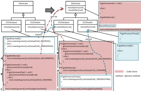
One of the earliest works on duplicate code refactoring was done by Tairas et al. [TG12], who developed an Eclipse Plug-in named CeDAR (Clone Detection,
Anal-ysis, and Refactoring). Their contribution falls in the three steps of removing dupli-cate code. The first step, Clone Detection is done by clone detection tools such
as CCFinder [KKI02], and NICAD [RC08a]. However, the results from these tools require pre-processing to get correct start-end line numbers for the clone fragments before they can be processed. For example, CCFinder reports clones as ranges of to-kens, whereas other tools might report incomplete statements. Therefore, their first contribution is parsing and integrating the output from clone detection tools into the refactoring process.
The output from Clone Detectionis used as an input for the Clone Analysis
step. Previous techniques help in finding opportunities for refactoring by examining some properties automatically, such as if the clones belong to classes within the same inheritance hierarchy [Kon01]. The limitation of these techniques are: 1) They will
find refactorable and non-refactorable clones, and 2) The decision is left to developers or maintainers to apply the refactoring manually. To overcome the first limitation in finding only refactorable clone groups, CeDAR employs the Eclipse IDE refactoring engine to check if the group of clones meets a set of preconditions for the Extract Method refactoring, i.e., extracting the clone fragments into a common method.
The last step is Refactoring, which is also done by the Eclipse IDE
refactor-ing engine. However, the Eclipse refactorrefactor-ing engine was not able to parameterize differences within the clone fragments, with the exception of differences in variable identifiers. CeDAR overcomes this limitation by extending the Eclipse refactoring engine to add support for method call and field access parameterization.
The evaluation of CeDAR was performed by comparing it to the Extract Method refactoring provided by Eclipse. They did an experiment on nine projects (including Apache Ant, JFreeChart, JEdit, and JRuby), and they used the clones reported by Deckard [Jia+07]. However, some of the groups were removed using the clone analysis results from ARIES [HKI08], and SUPREMO [Kon01], as they could not be refactored through extract method. ARIES and SUPREMO are tools used to evaluate and propose how clones can be refactored. The total number of groups they examined in their experiment is 1206. Eclipse was able to refactor 128 (10.6%), and CeDAR 226 (18.7%) of the total groups. The main limitation of their work is that it supports the refactoring of Type-I and simple Type-II clones only. Furthermore, the refactoring support is limited to clones located within the same Java file.
Meng et al. [Men+15] developed a fully automated refactoring tool, called RASE
that uses the abstract edit script generated by LASE [MKM13]. The edit script
is computed by comparing different versions of the same method and returning the differences as AST node insert, delete, update and move operations. Figure 3.4 shows
an example of edit scripts, where the lines in blue are added statements, in red are deleted statements, and in black are unchanged statements across versions. RASE
finds next the common changes in all methods (clones) and creates a generalized program transformation, called abstract edit script. RASE requires the clones to be
adjacent, so that it can generate a single AST node (and all its child sub-trees), or multiple sub-trees under same parent after theMerge step is performed.
pairs and 67% method groups. Systematic edits thus are a good clue for refactoring, rather than being obviated by method-level refactoring. However, RASEcannot automate refactoring in 46% of pairs and 33% of groups mainly because of language limitations, semantic constraints, and lack of common code. We manually checked software version histories after system-atic edits and found that in many cases, systemsystem-atically edited methods are not refactored. They either co-evolve, diverge, or stay unchanged. Our tool evaluation and software repository observations indicate that both automated systematic editing and refactoring are necessary to support software evolution.
This paper designs and implements an automated clone removal refactoring algorithm and demonstrates refactoring feasibility. Predicting refactoringdesirabilityis a hard problem because it depends on complex factors, such as code read-ability, the frequency and types of changes, future changes in requirements, and code size. Since RASE automates the feasibility step and quantifies code size impact, it should help developers determine refactoring desirability [4, 28, 33] and help with cost and benefit analysis [22, 26, 34], but we leave that investigation to future work.
In summary, this paper makes the following contributions. • We design and implement RASE, an advanced automated clone removal tool. It takes methods with systematic edits as inputs and fully automates refactoring to extract com-mon code with variations in types, methods, variables, and expressions.
• Evaluation on real-world pairs and groups of methods shows that RASEeffectively automates clone removal in many cases. This tool evaluation together with our manual software repository examination reveals that refactoring is not always applicable or actually applied to every sys-tematically edited method. Thus, automated refactoring is unlikely to obviate systematic editing.
• Previous studies find that clone refactoring is not neces-sary or feasible, but they did not construct an automated refactoring tool [1, 5, 8, 16, 17]. The lack of automa-tion introduces potential subjectivity bias. By automating refactoring, our study improves on the prior methodology and shows that refactoring is often feasible.
II. MOTIVATINGEXAMPLE
This section overviews our approach with an example based
on org.eclipse.compare.CompareEditorInputrevisions
v-20061120 and v20061218. Figure 1 shows a systematic edit on two methods. The unchanged code is in black, added code is inbluewith ‘+’, and deleted code is in red with ‘ ’. The two methods perform very similar input processing and experience similar edits: adding a variable declaration and updating statements. However, the changes involve using
different type, method, and variable names: IActionBars
vs. ISLocator; getActionBars vs. getServiceLocator;
findActionBars vs. findSite; offset vs. offset2; and
1. public class CompareEditorInput{
2. private ICompareContainer fContainer;
3. private boolean fContainerProvided;
4. private Splitter fComposite;
5. public IActionBars getActionBars (int offset){
6. if (offset == -1)
7. return null;
8.- if (fContainer == null){
9.+ IActionBars actionBars = fContainer.getActionBars();
10.+ if (actionBars==null&&offset!=0&&!fContainerProvided){
11. return Utilities.findActionBars(fComposite, offset);
12. }
13.- return fContainer.getActionBars();
14.+ return actionBars;
15. }
16. public ISLocator getServiceLocator (int offset2){
17.- if (fContainer == null){
18.+ ISLocator sLocator = fContainer.getServiceLocator();
19.+ if(sLocator == null&&offset2!=0&&!fContainerProvided){
20. return Utilities.findSite(fComposite, offset2);
21. }
22.- return fContainer.getServiceLocator();
23.+ return sLocator;
24. }
25.}
Fig. 1. An example of systematic changes based on org.eclipse.compare.-CompareEditorInputfrom revisions v20061120 and v20061218
1. … …method_declaration(… …) {!
2. … …!
3. INSERT: T$0 v$0 = fContainer.m$0(); !
4. UPDATE: if (fContainer == null) {! !
5. TO: if (v$0==null && v$1!=0 && !fContainerProvided){!
6. … …!
7. } !
8. UPDATE: return fContainer.m$0();! !
9. TO: return v$0;!
10.}
Fig. 2. Abstract edit script inferred by LASE
1. T$0 v$0 = fContainer.m$0();
2. if (v$0==null && v$1!=0 && !fContainerProvided){
3. return Utilities.m$1(fComposite, v$1);
4. }
5. return v$0;
Fig. 3. Abstract refactoring template of common code created by RASE
The script describes abstractly the edit applied to both meth-ods. It represents edit operations with AST node inserts, updates, moves, and deletes. Figure 2 shows the inferred abstract edit script for this example.
Given an edit script, RASE identifies edited statements related to the systematic changes. It uses the ranges of edits to scope its automated factorization and generalization, extracting the maximum common contiguous clone which encompasses all systematically edited statements. If similar edits are sur-rounded by cloned statements, RASE expands the refactoring scope to the entire method. For our example, in Figure 1, RASEselects lines 9-12, 14, 18-21, and 23 to refactor. Note that RASEincludes the unchanged lines 11-12 and 20-21 in order to extract syntactically validifstatements.
Next, RASEcreates an abstract refactoring template for the selected code snippets by matching expressions and identifiers between them, as shown in Figure 3. It uses the original code when identifiers or expressions are identical and otherwise
Figure 3.4: Example of systematic edit (Figure 1, Page 2 Meng et al. [Men+15]) Their approach consists of three steps: In t
![Figure 2.8: Change in execution behavior (Figure 5. in Tsantalis et al. [TMK15])](https://thumb-us.123doks.com/thumbv2/123dok_us/789779.2599845/38.918.160.768.238.598/figure-change-execution-behavior-figure-tsantalis-et-tmk.webp)