Sampling Strategy for Multi Spectral Image Classification Using
3-D-DWT and Morphological Profile
P.Bharathi
Mepco Schlenk Engineering College, Sivakasi, TamilNadu, India. [email protected]
Dr.S.Rajesh
Mepco Schlenk Engineering College, Sivakasi, TamilNadu, India. [email protected]
Abstract
Nowadays, Spectral-spatial processing has been used in multispectral image classification. In general, we select the training and testing samples randomly from the image. This method leads to overlap between the training and testing samples i.e the training and testing samples are sometimes same. This will give overlap between training and testing samples. To prevent this problem, we propose a controlled random sampling strategy for spectral-spatial methods. It can substantially reduce the overlap between training and testing samples and gives accurate evaluation. The overlap between the training and testing samples enriched by spatial information methods such as morphological profile and spatial filtering. The random sampling method is not right to access the spectral-spatial classification algorithms, since it is difficult to find the improvement of classification accuracy is originated by increasing the overlap between the training and testing samples.
Keywords experimental setting, multispectral image classification, random sampling, spectral-spatial processing.
INTRODUCTION
Remote sensing is the learning of information about an object without making physical contact with the object. During past several years, the sp ectral-spatial processing has attracted increasing attentions. By developing a variety of spectral-spatial methods, a large portion of the multispectral remote sensing community has focused their research on improving classification accuracy.
The spectral processing are improperly used in the context of spectral-spatial processing, leading to biased performance evaluation. This is especially when training and testing samples are randomly drawn from the same image.
It leads to overlap between the training and testing samples.
Spectral-spatial multispectral image classification system built on a supervised learning method is given in Figure.1.Training and testing samples are select from an image data set accompanying specific sampling method. The preprocessing step will be done. After the preprocessing step, the spectral spatial feature extraction is done.
The extracted features are given to machine learning algorithm and train a classifier. In the testing step, the learned classifier is used to predict the classes of testing samples.
Fig.1. Architecture of spectral-spatial multispectral image classification
In multispectral data set the training and testing samples are not given. For this purpose a sampling strategy is used to create the training and testing sets [1]. The stratified random sampling is often used for the sampling method [2]. To guarantee each class having sufficient samples, it first groups those labeled samples into subsets based on their class labels, and then, random sampling is carried out within each subset. In terms of the number of training samples in each subset, it normally requires that the proportion of each group should be the same as in the population. Then, the rest of samples are treated as testing samples in the testing step. This method is very simple to implement and statistical significance. In this paper, the relationship between the sampling strategies and the spectral-spatial processing in multispectral image classification, when the same image is used for training and testing is studied. In order to overcome the overlap between training and testing samples, we propose a controlled random sampling strategy. The contribution of this paper is as follows: First, The random sampling from the same
image experimental setting is not suitable for supervised spectral-spatial classification methods. Secondly, we find that under the random sampling setting, spectral-spatial methods can enhance the data dependence and improve the classification accuracy. Finally, we propose a novel controlled random sampling strategy which can substantially reduce the overlap between training and testing samples caused by spatial processing.
The rest of this paper is considered as follows. Module 2 reviews the spectral-spatial processing that have been commonly used for multispectral image classification. Module 3 reviews the spatial information submerged in the spectral-spatial processing under the experimental setting with random sampling is discussed. Module 4 analyzes the overlap between neighboring training and testing samples caused by spatial operations. Module 5 discusses the proposed controlled random sampling strategy. Module 6 reviews the experiments. Module 7 reviews the comparison study. Conclusions are discussed in Module 8.
SPECTRAL-SPATIAL PROCESSING
IN MULTISPECTRAL IMAGE
CLASSIFICATION
The spectral-spatial processing in multispectral image classification is discussed in this section. The spatial information defines to where a pixel locates in the image. Normally, spectral-spatial information can given to multispectral image classification through three ways. First, the image preprocessing is done and it can be used for image denoising, morphology and segmentation. Random noises in the image will be removed using image denoising. Several approaches have been utilized for this purpose, for example, smoothing filters, wavelet shrinkage and sparse coding
methods [3].In mathematical morphology, operations are done to extract spatial structures of objects depending to their spectral responses [4].
Second one is that feature extraction stage. The spectral features are extracted at a single pixel level in multispectral images. The spectral-spatial feature extraction methods use spatial neighborhood to calculate features. Typical examples include texture features, such as 3-D discrete wavelet [5], 3-D Gabor wavelet [6], 3-D scattering wavelet [7], and local binary patterns. Morphological profiles uses closing, opening, and geodesic operators to increase the spatial structures of objects.
Third, the image classification methods turn on spatial relation between pixels for model building. The method of doing is to calculate the similarity between a pixel and its surrounding pixels [8]. Similar spatial structures are explored in conditional random fields and multistate analysis [9]. The spatial information can also be traverse in building composite kernels in support vector machines (SVMs) [10]. While supervised learning approaches, such as K-nearest neighbors (KNNs), linear discriminant analysis, Bayesian analysis, SVMs, and so on, are widely used in these classification tasks [11].
SPATIAL INFORMATION
SUBMERGED
IN RANDOM SAMPLING
In this section, we discussed about the spatial information submerged in random sampling. In most cases, if random sampling is used for selecting training and testing samples in the same image, the class label of a testing sample can be easily inferred only by its spatial relation with the training samples. The training samples are sampled from the dataset based on the sampling rate as
5%,10%,25%. When the sampling rate comes to 25% ,the training samples is similar to the shape of ground truth map of the image.
The spatial coordinates were used as the spatial feature. The parameters of the SVM were learned via fivefold cross validation. Three sampling rates were given, i.e., 5%, 10%, and 25% to generate the training data from all labeled samples, while the rest of labeled data treated as the testing samples. When 5% of training samples are used, the spatial method achieves better accuracy. When it comes to 25% of sampling rate the classification accuracy reaches 100% for the spatial feature. While the spectral method has the lower accuracy when compared to spatial method. The sampling rate increases means the classification accuracy also increases on the dataset.
Fig 2 Kankaria area (size 300×300)
Fig 3. Ground truth of multispectral image
In summary, the random sampling from the same image makes an underestimated amount of spatial information be submerged in the training set and the testing set.
Study Area and Data Used
Figure.2shows the kankaria area of (size 300×300) which is located in Ahmedabad city in Gujarat, state of India. The land cover features of this study area include urban, vegetation, water body, waste land and hilly region, lakes, roadways.
It is very important to have the ground truth data which should form the training data set and on which the real classification can be performed and tested for the preparation of Ground Truth Data for a supervised method of classification. The Ground truth data of kankaria is shown in Figure. 3
OVERLAP BETWEEN TRAINING ANDTESTING DATA FROM THE SAME IMAGE
In this section the overlap between training and testing data from the same image is discussed. When it comes to the random sampling method, there is overlap between training and testing data. The training and testing samples are selected from the same image, their features are almost certain to overlap in the spatial domain because of the shared source of information. The random sampling provides a solution for data splitting and there is no overlap between training and testing samples. Nevertheless, the spectral-spatial methods usually exploit information from neighborhood pixels. This is normally implemented by a sliding window with a specific size, for example, 3 ×3, 5 ×5, etc. In each window, a filter is used to extract information. Overlap leads to using of the testing data for training purpose, and gives advantages to the spectral-spatial feature extraction methods. This ignore the principle of supervised learning that training and testing data shall not interact with each other. The feature is extracted by the spectral spatial features. The spectral spatial features is extracted by combining the spectral responses of pixels in a neighborhood. The discrete wavelet
transform is used to extract the texture feature based on spatial frequency analysis.
Experiment with Mean Filter-Based Spectral-Spatial Method
The experiment with mean filter based spectral spatial method is discussed. The features are formed by applying a mean filter to calculate the mean of the spectral responses in a neighborhood of the multispectral images, which was given as follows:
2 2 2 2 ) , ( 1 ) , ( A x A x i B y B y j j i s AB y x f (1)Where A and B are the width and height of neighborhoodsurrounding(x, y). We set the values for Aand Bbothfrom 1 up to 27 with an interval of 2. S(i, j ) represents thespectral response at location (i, j ) and f (x, y) is the feature extracted on location
(x, y), which contains both spectral andspatial information. If the sampling rate rises, the overlap also increases. When the size of filter is large, the overlap rate also increases rapidly.
The classification accuracy increases when the size of neighborhood increases, more testing provide to the training step. It is also interesting tosee that after the neighborhood increases to a specific size, the accuracy stops growing and tends to stable. This is because when the neighborhood becomes too large, samples from other classes are involvedin the feature extraction, which equalize the benefits ofoverlap.
Nonoverlap Measurement
Nonoverlap measurement gives the increase of classification accuracy. The feature includes more spatial information with larger filter size. To demonstrate how the spatial neighborhood influences the effectiveness of spectral-spatialfeature, we performed another experiment on those
testing samples not overlapped with the training data.
By using the larger filter size, the nonoverlap of testing samples classification accuracy does not increase. In overlap measurement the classification accuracy is increased when larger filter size is used. The filter-based spectral spatial feature extraction methods would make the training and testing samples overlap and then communicate with each other.
CONTROLLED RANDOM
SAMPLING STRATEGY
From the above discussion, the randomsampling from the same image is not suitable forevaluating the spectral-spatial methods. For that it is necessary to develop a new sampling strategy to separate the training and testing sets without overlap.Based on our analysis, theproblem of random sampling is that it makes the training and testing samples is same so it leads to overlap.
The proposed controlled random sampling method is used to create training and testing samples. Brief description of this method is given below.
First the image and sampling rate will be taken. Foreach class in the multispectral image, it selectsthe unconnected partitions for the each class and counts thesamples in each partition. This step is to find the spatial distribution of each class. For each partition, the trainingsamples are generated by extending region from the seed pixel.We used the idea of region growing to create region-shape training samples. On the ground truth map, the seed points are randomly selected from different partitions of classes to make the training samples. The partition is nothing but the group of connected pixels with the same labels.
The region growing method is used to grow the regions based on the seed point value similarity. Region is grown from the seed pixel by adding the neighbouring pixels that are similar. When the growth of one region grows means the another seed point is choosen which does not belong to any region. The process is repeated until the region grows.
After the above steps are applied to all classes, those samples in the grown regions with their labels are chosen, as the training samples and the rest of pixels work as the testing samples.
Algorithm 1 Controlled Random Sampling Strategy
1:Need: The Multispectral image J is taken
2:Different percentage of sampling rate ris taken from the multispectral image.
3:for each category c in multispectral image Jdo
4:choose all disconnected partitions M in the labelc
5:for each partition p in disconnected partitions M do
6:Compute the number of samples in the partition
7:Calculate the number of training samples in the partition by = × r
8:Perform region growing algorithm to grow the regions in the label.
9: In region growing algorithm, randomly choose a seed point din the partition
10:Applying the region-growing algorithm to extend the seed point dto a region
gwhose size is equal to 11:end for
12:Merge these regions gto get the training samples
13:end for
14:Merge the training samples and their corresponding class labels to get the whole training set R
EXPERIMENTS
The advantage of the proposed controlled random sampling against random sampling
is proved with experiments.The mean filter and Gaussian filters are used for preprocessing purpose. We havedeveloped an experiments to test these two strategieswhen they are used to evaluate spectral-spatial operations indifferent stages of image classification. The spectral spatial feature extraction methods such as 3-D-DWT and Morphological profile are compared using the sampling methods. Raw Spectral Feature
In this experiment the comparison of controlled random sampling method and random sampling when raw spectral features are used. When the sampling rate is high, the classification accuracy is increased in the dataset. There is reduction in the classification accuracy when the controlled random sampling method is used. The testing samples are far away from the training regions are misclassified in controlled random sampling method compared with random sampling method. Therefore the proposed method made the hyperspectral classification a challenging problem to the feature extraction.
Spectral-Spatial Features
To test the proposed sampling method with two typical spectral-spatial feature extraction methods, i.e., 3-D DWT and morphological profile.
Three-Dimensional Discrete Wavelet Transform:
The DWT is derived from the wavelet transform provides mathematical tools for time-scale signal analysis in the similar way as the short time fourier transform (STFT) in the time-frequency domain. DWT is implemented by a series of filters in the frequency domain. The multispectral images has three dimensions, the features are extracted by the DWT.The 3-D-DWT is a combination of 1-D-3-D-DWT in x,y,z directions.
Fig.4 shows the single level 3-D-DWT
First, the multispectral image was processed by a cascade of high-pass filters and low-pass filters. Figure 4 shows the decomposition tree for single level 3-D-DWT,the volume data are decomposed into eight subbands, i.e., LLL, LLH, LHL, LHH, HLL, HLH, HHL and HHH. In each level, the data were decomposed into high-frequency part and low-high-frequency part. After three levels of decomposition, theoriginal data were separated into 15 subcubesL1,L2, . . . ,L15 based on the bandwidth.To further capture the spatial distribution of multispectral images, a mean filter was applied on the subcubes
̂ ( ) ∑ ∑ ( )
(2)
Then, these subcubes were concatenated into the wavelet features. Figure 5 shows the three level decomposition of dataset.The multidimensional function was carried out along two spatial dimensions x
and y, as well as the spectral dimension λ, respectively. The final concatenation worked as the feature for the whole data cube and can be represented as
( ) ( ̂ ̂ ̂ , ̂ , ̂ ,…, ̂ ̂ ̂ ̂ ) (3)
Where f (x, y) is the 3-D-DWT feature at location (x,y)
Fig 5: Three level decomposition of multispectral image
Morphological Profile
Morphological operations consist of some basic operators. The operators include erosion and dilation, which expandsand shrinks the structures, respectively. Erosion removes the pixels to the boundaries of object in an image depending on the structuring element. While dilation adds the pixels to the boundaries of object in an image depending on the structuring element. This result of processing are known as morphological profile. The spatial feature extraction are as follows:
( )( )
( )( ) ( )( ) ( )( ) ( )( )] (4)
where ( )( )and ( )( ) were the opening and closing operations with a disk-shaped structural element of size n, respectively. Before the feature extraction, a principle component analysis step was applied to multispectral images to reduce the dimension of the data. Then, the morphological profiles were obtained on each of the m primary components
̂( )( ) ( )( ) ( )( ) …, ( )( )
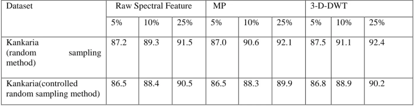
](5) In the last step, the morphological profiles were stacked with the spectral response to form the spectral-spatial feature. Table I shows the classification accuracies of dataset with random sampling method and controlled random sampling method using raw spectral feature,3-D-DWT and morphological profile. Figure 6 shows the classification accuracy based on 3-D-DWT,classification accuracy is lower for controlled sampling method compared with random sampling. In Table I,3-D-DWT achieves higher accuracy than MP when random sampling is adopted. When adopting the new sampling strategy, 3-D-DWT still performs slightly better than MP.
Table 1 Classification accuracies using 3-D-DWT, Morphological Profile and Raw Spectral Feature when linear SVM is used.
Dataset Raw Spectral Feature MP 3-D-DWT
5% 10% 25% 5% 10% 25% 5% 10% 25% Kankaria (random sampling method) 87.2 89.3 91.5 87.0 90.6 92.1 87.5 91.1 92.4 Kankaria(controlled random sampling method)
Fig 6 shows the classification accuracy of 3-D-DWT.
COMPARISON BETWEEN RANDOM SAMPLING AND CONTROLLED RANDOM SAMPLING METHOD To make the comparison and similarities between random sampling and controlled random sampling method, we calculated the percentage of overlap and classification accuracy using different sampling rate. The overlap between training samples and testing sampling for random sampling and controlled random sampling is similar. Figure 7 shows the comparison of overlap for both methods. The controlled random sampling method greatly reduced the overlap when comparing with random sampling when the training set becomes large.
Fig 7 shows the comparison of overlap
The training set is small means, the overlap between the training and testing sets is not much affected when spectral spatial operations involved. If the training set is increased the overlap between training and testing samples increases in
random sampling and the proposed method destroy such increase.
CONCLUSION
This paper presented a study of random sampling method to evaluate the spectral-spatial methods in multispectral image classification. The random sampling method has leads to some overlap between training and testing samples. We proposed the new sampling method to prevent this problem.
A controlled random sampling strategy is a new sampling method is used to reduce the overlap between training and testing samples for spectral and spatial methods compared with random sampling method. The classification accuracy is somewhat low compared with existing method because we defined the sampling rate to take the samples and region growing method is used to grow the pixels based on the seed points. The training and testing samples are separated based on the region growing method.
The advantage of the proposed method is even when the scale of the training set is large. Therefore, the new sampling method gives a proper way to evaluate the effectiveness of spectral-spatial operation. Furthermore, this methods are used in hyperspectral images. 80 85 90 95 5 10 15 20 25 class if icatio n ac cu rac y
percentage of sampling rate random sampling method
controlled random sampling method
0 0.2 0.4 0.6 0.8 1 5 10 15 20 25 perc ent a g e o f o v er la p training samples:percentage random sampling method controlled random sampling method
REFERENCES
1. S. V. Stehman and R. L. Czaplewski, “Design and analysis for thematicmap accuracy assessment: Fundamental principles,” Remote Sens. Environ.,vol. 64, no. 3, pp. 331–344, Jun. 1998. 2. J. A. Richards and X. Jia, Remote
Sensing Digital Image Analysis:An Introduction, D. E. Ricken and W. Gessner, Eds., 3rd ed. Secaucus,NJ, USA: Springer-Verlag, 1999.
3. M. Ye, Y. Qian, and J. Zhou, “Multitask sparse nonnegative matrixfactorization for joint spectral– spatial multispectral imagery denoising,”IEEE Trans. Geosci. Remote Sens., vol. 53, no. 5, pp. 2621– 2639,May 2015.
4. S. Velasco-Forero and J. Angulo, “Spatial structures detection in
hyperspectralimages using
mathematical morphology,” in Proc. 2nd WorkshopMultispectral Image Signal Process.,Evol. Remote Sens. (WHISPERS), Jun. 2010, pp. 1–4. 5. Y. Qian, M. Ye, and J. Zhou,
“Hyperspectral image classification basedon structured sparse logistic regression and three-dimensional wavelettexture features,” IEEE Trans. Geosci. Remote Sens., vol. 51, no. 4,pp. 2276–2291, Apr. 2013.
6. S. Jia, L. Shen, and Q. Li, “Gabor feature-based collaborative representationfor hyperspectral imagery classification,” IEEE Trans.
Geosci.Remote Sens., vol. 53, no. 2, pp. 1118–1129, Feb. 2015.
7. Y. Tang, Y. Lu, and H. Yuan,
“Hyperspectral image
classificationbased on three-dimensional scattering wavelet transform,” IEEE Trans.Geosci. Remote Sens., vol. 53, no. 5, pp. 2467– 2480, May 2015.
8. H. Pu, Z. Chen, B. Wang, and G.-M. Jiang, “A novel spatial–spectral similarity measure for dimensionality reduction and classification of hyperspectral imagery,” IEEE Trans. Geosci. Remote Sens., vol. 52,no. 11, pp. 7008–7022, Nov. 2014.
9. L. Fang, S. Li, X. Kang, and J. A. Benediktsson, “Spectral–spatial hyperspectral image classification via multiscale adaptive sparse representation,” IEEE Trans. Geosci. Remote Sens., vol. 52, no. 12, pp. 7738–7749, Dec. 2014.
10. G. Camps-Valls, L. Gomez-Chova, J. Munoz-Mari, J. Vila-Frances, and J. Calpe-Maravilla, “Composite kernels for hyperspectral image classification,”
IEEE Geosci. Remote Sens. Lett., vol. 3, no. 1, pp. 93–97,Jan. 2006.
11. J. M. Bioucas-Dias, A. Plaza, G. Camps-Valls, P. Scheunders,N. M. Nasrabadi, and J. Chanussot, “Hyperspectral remote sensing data analysis and future challenges,” IEEE Geosci. Remote Sens. Mag., vol. 1,no. 2, pp. 6–36, Jun. 2013.