C.D. Howe Institute
COMMENTARY
Energy Prices and Alberta
Government Revenue Volatility
Stuart Landon and Constance Smith
In this issue...
How to stabalize Alberta’s wild revenue and spending path.
The Alberta government is heavily exposed to energy price volatility, as the province relies to a great extent on revenues derived from the production of oil and natural gas. Energy prices change substantially and unpredictably, causing large and uncertain movements in revenues. Adjusting to these movements typically involves economic, social, and political costs. Alberta’s revenues are considerably more volatile than the revenues of other provinces because of Alberta’s greater dependence on energy-related revenues and the high volatility of these revenues. One way to reduce the volatility of revenues is to diversify the tax base –through, for example, the use of a sales tax. But that method would have a small effect on overall revenue volatility since Alberta’s resource revenues are such a large share of total own-source revenues. Another method would be to smooth revenue, using futures and options markets, but that approach could be expensive and politically risky, and would not eliminate all revenue volatility.
The best option is a resource revenue stabilization fund. Such a fund would reduce revenue volatility in Alberta significantly. It would lead to greater revenue stability because the money it would contribute to the budget in any particular year would be based on revenues averaged over prior years. A stabilization fund also would reduce uncertainty, since current revenue would depend on known past contributions to the fund. Key characteristics that would increase the probability of a stabilization fund’s success are its simplicity, transparency, and a gradual transition to full implementation.
ABOUT THEINSTITUTE
The C.D. Howe Instituteis a leading independent, economic and social policy research institution. The Institute promotes sound policies in these fields for all Canadians through its research and communications. Its nationwide activities include regular policy roundtables and presentations by policy staff in major regional centres, as well as before parliamentary committees. The Institute’s individual and corporate members are drawn from business, universities and the professions across the country.
INDEPENDENT• REASONED• RELEVANT
T
HEA
UTHORSOF
T
HISI
SSUESTUART LANDON is Professor of Economics at the University of Alberta. CONSTANCE SMITH is Professor of Economics at the University of Alberta.
Rigorous external review of every major policy study, undertaken by academics and outside experts, helps ensure the quality, integrity and objectivity of the Institute’s research.
$12.00
ISBN 978-0-88806-820-4 ISSN 0824-8001 (print); ISSN 1703-0765 (online)
O
il and natural gas prices often
change rapidly, substantially,
and unpredictably.
The Alberta government is heavily exposed to energy price volatility because it relies to a large extent on revenue derived from the production of oil and natural gas. For Alberta, as for the governments of other energy-producing jurisdictions, adjusting to large revenue
movements typically involves economic, social, and political costs. Rapid declines in energy revenues can lead to pressure for cuts in expenditures that are difficult to accomplish quickly and efficiently. Revenue volatility that drives government expenditures
can also cause fiscal policy to be procyclical, thus magnifying movements in economic activity.
This paper provides an analysis of the volatility of Alberta government revenues and possible methods of dealing with this volatility. Alberta’s revenues are considerably more variable than those of other provinces; importantly, however, the volatility of Alberta’s own-source revenues less resource revenues is similar to that of other provinces.
One commonly proposed method to reduce the volatility of revenues is tax base diversification, through the use of, say, a sales tax. We show, however, that this approach would have a
relatively small effect on overall revenue volatility since Alberta’s resource revenues are such a large share of own-source revenues. Other alternatives, such as revenue smoothing using futures and options markets, can be expensive, are associated with significant political risks, and cannot
eliminate all revenue volatility. Movements of the exchange rate are another source of revenue stabilization, since the Canadian dollar tends to appreciate when energy prices rise and to depreciate when they fall, but this effect is relatively small.
An effective approach to address revenue volatility is to establish a resource revenue
stabilization fund with fixed contribution and withdrawal rates. A simulation using Alberta data for the past 30 years shows that this form of stabilization fund would lead to greater revenue stability, both because a large fixed fraction of volatile resource revenues would be deposited in the fund and because the revenue contributed to the budget from the fund in any particular year would depend on contributions to the fund in all previous years. Revenue uncertainty also would be reduced with a stabilization fund since future revenue would depend on known past contributions. In comparison, the Alberta Heritage Savings Trust Fund’s ability to stabilize revenues is quite limited: when the fund was established, it received a fixed percentage of resource revenues each year, but this practice was ended in 1987, although the fund has received ad hoc contributions from general revenues in several recent years (Alberta 2010b).
Problems with Revenue Volatility
Government revenue volatility can have important negative consequences. A government that wishes to provide infrastructure and social services at a level that is sustainable in the longer term will have difficulty setting the appropriate level of spending when it is not clear what part of volatile revenue changes is permanent and what part is temporary. Revenue volatility can also make it more difficult for a government to put in place long-term plans if volatility undermines the government’s credibility in terms of its ability accurately to forecast and manage revenues (Tuer 2002, 25). The two provinces most heavily reliant on volatile energy revenues, Alberta and Saskatchewan, have the worst records at
hitting budget targets (Busby and Robson 2010). Revenue volatility also makes it more difficult for the private sector to predict future government tax and spending policies, which could have important consequences for private-sector investment decisions, leading to slower economic The authors received helpful comments on an earlier draft from Ken Boessenkool, Colin Busby, Ben Dachis, Bev Dahlby, Herb Emery, Mel McMillan, Barry Scholnick. However, the authors retain sole responsibility for any errors. An earlier version of this paper was presented at a C.D. Howe Institute and University of Alberta Institute for Public Economics Conference on May 6th and 7th, 2010.
growth (Barnett and Ossowski 2002; Afonso and Furceri 2008; Sturm, Gurtner, and Alegre 2009).
Another major consequence of revenue
volatility is that, in many jurisdictions, it induces volatile movements in government spending. When revenues expand during a boom,
expenditures tend to grow, but when revenues fall, expenditures are cut, although often more slowly than expenditures initially rose.1 That is, revenue volatility can cause governments to pursue stop-go procyclical fiscal policies (Sturm, Gurtner, and Alegre 2009). These procyclical policies accentuate the effects of economic cycles so that, rather than acting to reduce volatility, the government becomes a driving force magnifying output fluctuations. The volatility of economic activity and the volatile provision of government services then reduce individual welfare if consumers prefer less variable income and consumption. Further, given the real costs of moving resources between expanding and contracting sectors, it is especially important for government policy to help stabilize the economy, rather than to aggravate economic volatility.
Government spending increases during revenue booms compete with private-sector spending, which can raise wages and other input costs, thereby increasing both public and private-sector costs. There is some indication that increases in government revenues are correlated with upward pressure on prices. In Alberta, for example, the prices of current goods and services purchased by government rose at an average annual rate of 4.1 percent between 2002 and 2008, while they rose by only 2.6 percent in British Columbia and 3.3 percent in Ontario. During this same period, real per capita government revenues rose more than
twice as fast in Alberta as in either Ontario or British Columbia.
Large increases in government revenues during booms also can lead governments to spend on services and investment projects that have
relatively low returns. In turn, the rapid expansion of programs and capital spending during revenue booms can stretch the capacity of governments to provide services and monitor spending, leading to waste, inefficiency, and the unproductive use of government funds (Barnett and Ossowski 2002). Further, during a revenue collapse, it is difficult to cut spending efficiently –that is, to cut first those projects and services with the lowest taxpayer benefit. Large spending cuts precipitated by a fall in revenues also can damage the morale and capacity of the public sector, leading to the more inefficient provision of public services.
To the extent that it is easier politically to raise government spending than to reduce it, there might be a greater tendency to expand spending in revenue booms than to contract spending in busts. Thus, revenue volatility can result in an expansion of the size of government and, potentially, the implementation of an unsustainable fiscal plan that necessitates even greater expenditure cuts in the future.2
The Volatility of Alberta Government Revenues3
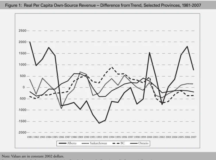
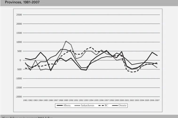
The Alberta government’s own-source revenues –
total revenues less transfers from other levels of government –are quite volatile relative to those of the other provinces (see Figure 1).4 Over the period from 1982 to 2007, the year-to-year change in Alberta’s real per capita own-source revenues exceeded 10 percent nine times. In 1 For example, Busby and Robson (2010) find a significant and large positive correlation between within-year Alberta government spending
adjustments and deviations of revenues from budget projections.
2 Kneebone and McKenzie (2000) report that, over the 1962-93 period, unexpected increases in revenues tended to be treated as permanent by Alberta budgetmakers and to lead to expenditure increases, while unexpected decreases tended to be treated as temporary, causing no corresponding spending reduction. Interviews reported by Boothe (1995) support these results.
3 Sources and definitions for the data used in the text, figures and tables are given in the Data Appendix.
4 Revenue volatility depends on both movements in tax bases and changes in tax rates. Due to difficulties with obtaining data on different tax rates through time, for the most part the analysis focuses on revenue volatility and does not distinguish whether this volatility is due to tax base or tax rate volatility.
comparison, this magnitude of revenue change occurred on only six occasions in Saskatchewan, only once in British Columbia, and not at all in Ontario.
A useful way to compare revenue volatility is to examine the coefficient of variation. This commonly used measure of volatility is the standard deviation (the square root of the variance) divided by the mean.5 The advantage of this measure over others, such as the standard deviation, is that its value does not depend on the units by which a variable is measured. This is desirable since government per capita revenues often differ greatly across provinces and revenue
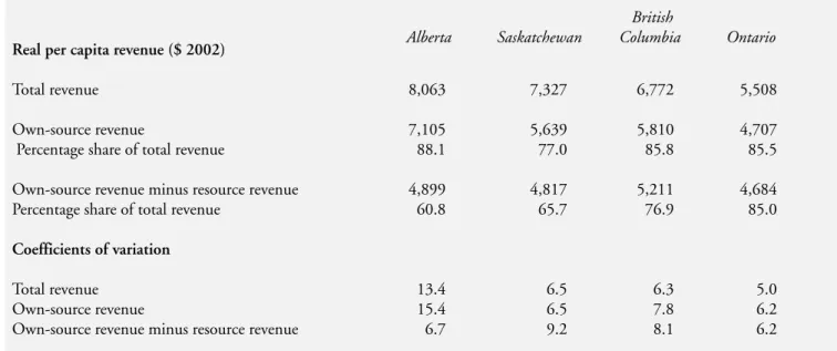
types. For the period 1981-2007, the coefficient of variation for Alberta government real per capita own-source revenues is 15.4, while for British Columbia, Saskatchewan, and Ontario the coefficients of variation are 7.8, 6.5, and 6.2, respectively (Table 1).6 Thus, Alberta’s own-source revenues were more than twice as variable as those of the other three provinces over that period. In dollar terms, these volatility values imply that a one standard deviation band around average real per capita own-source revenues for Alberta is $2,188, but only $906 for British Columbia.
5 Since government revenues grow through time, the standard deviation is calculated after de-trending. The ratio is also multiplied by 100 to put it in percentage terms.
6 Since the coefficients of variation are smaller for total revenues relative to those for own-source revenues, federal transfers have, on average over the period from 1981 to 2007, reduced revenue volatility.
-2000 -1500 -1000 -500 0 500 1000 1500 2000 2500 1981 1982 1983 1984 1985 1986 1987 1988 1989 1990 1991 1992 1993 1994 1995 1996 1997 1998 1999 2000 2001 2002 2003 2004 2005 2006 2007
Alberta Saskatchewan BC Ontario
Note: Values are in constant 2002 dollars.
Source: Authors’ calculations using Statistics Canada data; see the Data Appendix for more information.
The Causes of Alberta’s Revenue Volatility
The greater variability of Alberta government revenues is driven principally by the highly volatile energy sector resource component of revenues and, to a much smaller extent, by the volatility of corporate profits (see Figure 2 and Table 2). Volatility in these revenue sources, in turn, is driven mainly by movements in energy prices. The Magnitude and Volatility of Alberta’s Resource Revenues
For Alberta, the simple correlation between the growth rate (the year-to-year percentage change) of real per capita total own-source revenues and the growth rate of resource revenues was 0.90 over the period from 1982 to 2007 (Table 3).7 The growth rate of corporate tax revenues had the next highest correlation with own-source revenues, at 0.71. In contrast, for personal income taxes, the second-largest tax source in Alberta, the correlation with own-source revenues was only 0.42 over the period. In the other provinces, own-source
revenues were less correlated with resource revenues and, in general, more highly correlated with personal income tax revenues.
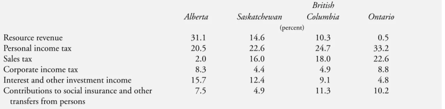
One reason for the large impact of resource revenue volatility on Alberta’s own-source revenue volatility is that resource revenues are the largest single component of the province’s own-source revenues, accounting, on average, for 31 percent of real per capita own-source revenues from 1981 to 2007; the next-largest revenue type, personal income taxes, accounted for only 20.5 percent. As Table 4 shows, the share of resource revenues in Alberta’s own-source revenues is large relative to other provinces. Resource revenues made up only 14.6 percent of Saskatchewan’s own-source revenues over the 1981 to 2007 period and were the province’s third-largest revenue source, after personal income taxes and the retail sales tax. In British Columbia, resource revenues were only 10.3 percent of revenues and the fourth-largest revenue type, while in Ontario resource revenues were an insignificant component of own-source revenues.
Not only are resource revenues by far the largest component of government revenues in Alberta, 7 To represent resource revenues here, we used "royalties" as designated by Statistics Canada; these revenues include Crown lease payments,
but not "miscellaneous taxes on natural resources."
Real per capita revenue ($ 2002)
Total revenue 8,063 7,327 6,772 5,508
Own-source revenue 7,105 5,639 5,810 4,707
Percentage share of total revenue 88.1 77.0 85.8 85.5 Own-source revenue minus resource revenue 4,899 4,817 5,211 4,684 Percentage share of total revenue 60.8 65.7 76.9 85.0
Coefficients of variation
Total revenue 13.4 6.5 6.3 5.0
Own-source revenue 15.4 6.5 7.8 6.2
Own-source revenue minus resource revenue 6.7 9.2 8.1 6.2
Table 1: Average Real Per Capita Revenue and Volatility, Selected Provinces, 1981-2007
Note: The coefficient of variation, a measure of volatility, is the ratio (multiplied by 100) of the standard deviation of the differences from an exponential trend to the average value of the series.
Source: Authors’ calculations using Statistics Canada data; see the Data Appendix for more information.
British
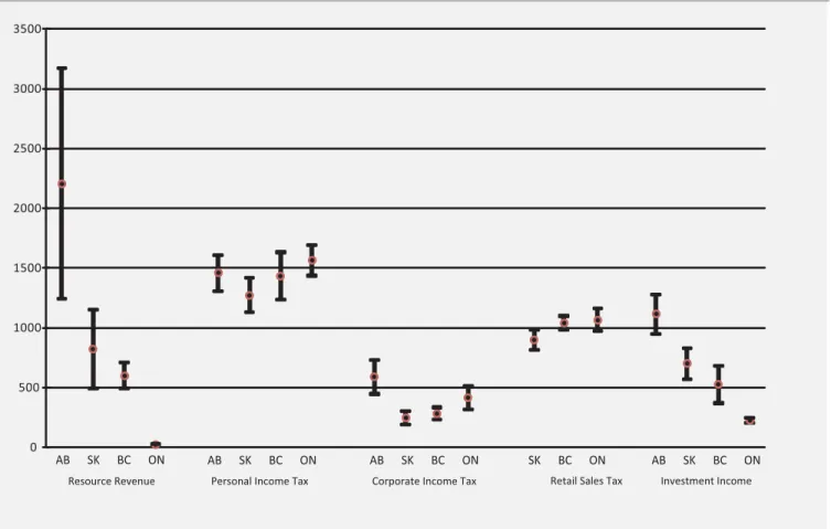
they are also the most variable. The coefficient of variation associated with resource revenues in Alberta over the period from 1981 to 2007 is 43.6 (Table 2).8 A one standard deviation band around $2,208 –the average value of real per capita resource revenues –ranges from $1,245 to $3,169. The magnitude of this band, $1,924, is equivalent to 27 percent of average own-source revenues. In comparison, corporate income taxes, the second-most-variable component of revenues, with a coefficient of variation of 24.2, have a one standard deviation band of only $284.
The volatility of resource revenues is due
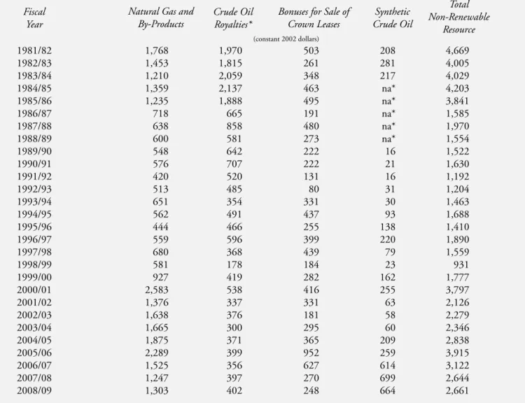
primarily to variation in energy prices, particularly the price of natural gas, which accounted for 45 percent of total resource receipts from 1981 to
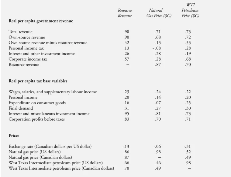
2009 and 54 percent over the past five years (Table 5). Over the period from 1982 to 2007, the correlation between the growth rate of real per capita resource revenues and the growth rate of the real Canadian dollar price of natural gas is 0.87. Changes in this price also drove changes in total real per capita own-source revenues: the correlation between the growth rate of real per capita own-source revenues and the real Canadian dollar natural gas price is 0.68. In comparison, the correlation between changes in real per capita own-source revenues less resource revenues and changes in the real natural gas price is only 0.13. The correlations for West Texas Intermediate (WTI) petroleum are similar to those for natural gas (Table 6). Given the volatility of energy prices 8 This level of variability is not unique to Alberta but is similar in magnitude to the export revenue volatility of 21 major petroleum exporters
reported in Borensztein, Jeanne, and Sandri (2009).
0 500 1000 1500 2000 2500 3000 3500 AB SK BC ON AB SK BC ON AB SK BC ON SK BC ON AB SK BC ON
Resource Revenue Personal Income Tax Corporate Income Tax Retail Sales Tax Investment Income
Note: Values are in constant 2002 dollars.
Source: Authors’ calculations using Statistics Canada data; see the Data Appendix for more information.
Figure 2: Average Real Per Capita Revenue and One Standard Deviation Band, Selected Provinces, 1981-2007
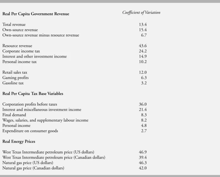
and the close relationship between resource revenues and energy prices, it is not surprising that resource revenues are quite volatile. The coefficients of variation over the period from 1981 to 2007 of the real Canadian dollar prices of natural gas and WTI petroleum are 42.0 and 39.4, respectively. This level of volatility is similar to that of resource revenues, while the volatility of other tax bases tends to be much smaller –for example, the volatility measure for personal income, the tax base for the personal income tax, is just 4.8 (Table 2).
Much of the volatility of Alberta government revenues has been driven by persistent movements
away from trend. As Figure 1 above shows, real per capita own-source revenues were above trend from 1981 to 1985, below trend from 1986 through 1999, above trend in 2000 and 2001, below in 2002, and above trend from 2003 through 2007. The longer-term movements in revenues away from trend are driven by
movements in resource revenues, as own-source revenues minus resource revenues move above and below trend twice as often as total own-source revenues (Figure 3). The persistence of revenue movements above and below trend are important because they imply that downturns in revenues might not be short lived, while upturns might
Table 2: Volatility of Government Revenue and Selected Tax Bases, Alberta, 1981-2007 Real Per Capita Government Revenue
Total revenue 13.4
Own-source revenue 15.4
Own-source revenue minus resource revenue 6.7
Resource revenue 43.6
Corporate income tax 24.2
Interest and other investment income 14.9
Personal income tax 10.2
Retail sales tax 12.0
Gaming profits 6.3
Gasoline tax 3.2
Real Per Capita Tax Base Variables
Corporation profits before taxes 36.0 Interest and miscellaneous investment income 21.4
Final demand 8.3
Wages, salaries, and supplementary labour income 8.2
Personal income 4.8
Expenditure on consumer goods 2.7
Real Energy Prices
West Texas Intermediate petroleum price (US dollars) 46.9 West Texas Intermediate petroleum price (Canadian dollars) 39.4 Natural gas price (US dollars) 46.3 Natural gas price (Canadian dollars) 42.0
Note: The coefficient of variation, a measure of volatility, is the ratio (multiplied by 100) of the standard deviation of the differences from an exponential trend to the average value of the series. The sample period for Alberta’s retail sales tax, gaming profits, and gasoline tax is 1994–2007, because the use of these taxes changed considerably in the late 1980s and early 1990s. The retail sales tax includes taxes on alcohol and tobacco only.
Source: Authors’ calculations using Statistics Canada data; see the Data Appendix for more information. Coefficient of Variation
seem permanent and, thereby, induce too great an increase in spending.
Considerable evidence suggests that movements in oil prices are persistent (Hamilton 2008). Given the dependence of resource revenues on energy prices, the long movements in own-source revenues away from trend can be attributed to this persistence. As a consequence, resource revenues have no tendency to converge quickly to some stable average value.
The Volatility of Non-Resource Revenues After resource revenues, corporate tax revenues are the most volatile revenue type in Alberta (Table 2). The coefficient of variation of Alberta’s real per capita corporate tax revenues for the period from 1981 to 2007 is 24.2, which is similar to the volatility of corporate tax revenues in both
Saskatchewan and Ontario. Although volatile, corporate tax revenues have not been a large driver of overall revenue volatility, since they accounted for only 8.3 percent of own-source revenues over the 1981-2007 period, or just one-quarter of the share of the more volatile resource component of revenues. In fact, the real per capita dollar value of the one standard deviation band around average corporate tax revenues is almost identical to that for the much less volatile revenues from personal income taxes because personal income taxes contributed a much larger share of total own-source revenues –20.5 percent on average. Nevertheless, both resource revenues and
corporate tax revenues are more highly correlated with energy prices than are personal income tax revenues.
Table 3: Correlation Coefficient between the Percentage Change in Total Own-Source Revenue and the Percentage Change in the Variable Indicated, Selected Provinces, 1982-2007
Note: Values for Alberta's retail sales tax and Ontario's resource revenue are not included because Alberta does not have a general retail sales tax that is comparable to the retail sales taxes in the other provinces, and Ontario's resource tax royalties are extremely small. Source: Authors’ calculations using Statistics Canada data; see the Data Appendix for more information.
Own-source revenue minus resource revenue .75 .86 .92 1.00
Resource revenue .90 .67 .59 –
Corporate income tax .71 .33 .46 .83
Personal income tax .42 .20 .66 .74
Retail sales taxes – .53 .49 .75
Table 4: Selected Revenue Types: Average Share of Real Per Capita Own-Source Revenue, Selected Provinces, 1981–2007
Note: Sales tax includes alcohol and tobacco taxes; Alberta has no general retail sales tax.
Source: Authors’ calculations using Statistics Canada data; see the Data Appendix for more information.
(percent)
Resource revenue 31.1 14.6 10.3 0.5
Personal income tax 20.5 22.6 24.7 33.2
Sales tax 2.0 16.0 18.0 22.6
Corporate income tax 8.3 4.4 4.9 8.8
Interest and other investment income 15.7 12.4 9.1 4.8 Contributions to social insurance and other 7.5 4.9 11.3 10.2
transfers from persons
British
Alberta Saskatchewan Columbia Ontario
British
Thus, movements in energy prices might cause synchronized movements in both types of tax revenues, accentuating the volatility
of total revenues (Table 6).
A comparison of the volatility of non-resource own-source revenues in Alberta and other provinces illustrates the importance of the role played by the volatility of resource payments in generating Alberta government revenue volatility. While the coefficient of variation of Alberta’s real per capita own-source revenues for the period from 1981 to 2007 is 15.4, the coefficient of variation of own-source revenues less resource
revenues is 6.7 (Table 1), only slightly higher than the corresponding measure for Ontario (6.2) and lower than those for British Columbia (8.1) and Saskatchewan (9.2). Hence, Alberta’s non-resource own-source revenues are, on average, similar in terms of volatility as those of the other provinces.
How to Reduce Revnue Volatility
Alberta government revenue volatility is driven primarily by resource revenue volatility, which, in turn, is driven by energy price volatility. Yet energy prices are determined in world or North
Table 5: Real Per Capita Natural Resource Revenue by Type, Alberta, Fiscal Years 1981/82-2008/09
*Crude oil royalties for 1984/85-1988/89 include synthetic crude products.
Sources: Revenues are from Alberta, Department of Energy, Annual Report, various issues. Data for population and the price index are from Statistics Canada as described in the Data Appendix. These population and price data are annual, so data are for the calendar year in which the fiscal year begins.
(constant 2002 dollars) 1981/82 1,768 1,970 503 208 4,669 1982/83 1,453 1,815 261 281 4,005 1983/84 1,210 2,059 348 217 4,029 1984/85 1,359 2,137 463 na* 4,203 1985/86 1,235 1,888 495 na* 3,841 1986/87 718 665 191 na* 1,585 1987/88 638 858 480 na* 1,970 1988/89 600 581 273 na* 1,554 1989/90 548 642 222 16 1,522 1990/91 576 707 222 21 1,630 1991/92 420 520 131 16 1,192 1992/93 513 485 80 31 1,204 1993/94 651 354 331 30 1,463 1994/95 562 491 437 93 1,688 1995/96 444 466 255 138 1,410 1996/97 559 596 399 220 1,890 1997/98 680 368 439 79 1,559 1998/99 581 178 184 23 931 1999/00 927 419 282 162 1,777 2000/01 2,583 538 416 255 3,797 2001/02 1,376 337 331 63 2,126 2002/03 1,638 376 181 58 2,279 2003/04 1,665 300 295 60 2,346 2004/05 1,875 371 365 209 2,838 2005/06 2,289 399 952 259 3,915 2006/07 1,525 356 627 614 3,122 2007/08 1,247 397 270 699 2,644 2008/09 1,303 402 248 664 2,661 Fiscal Year
Natural Gas and By-Products
Crude Oil Royalties*
Bonuses for Sale of Crown Leases Synthetic Crude Oil Total Non-Renewable Resource
American markets and effectively are out of the control of the Alberta government. How, then, could revenue volatility be reduced? Methods include limiting the influence of resource revenues on movements in overall revenues –say, by tax base “diversification” –hedging in futures or options markets, and using a stabilization fund. Tax Base Diversification
One method to reduce revenue volatility is to decrease the dependence of revenues on the more volatile energy-related tax bases through tax base diversification, which motivates suggestions that Alberta implement policies to diversify its
economy away from energy-related activities. Policies of this type, however, have three
shortcomings. First, such an approach could take a long time to yield results; second, it would run counter to Alberta’s comparative advantage – namely, the extraction of energy resources; and third, government-encouraged economic diversification relies on governments’ ability to pick successful non-energy-related industries, but there is little evidence that they can do this effectively.
Another way to reduce the dependence of total revenues on the energy sector is to collect less revenue from the more volatile energy-related tax bases: energy sector production (resource-based
Table 6: Correlation Coefficients between Annual Percentage Changes, Alberta, 1982-2007
Source: Authors’ calculations using Statistics Canada data; see the Data Appendix for more information.
Real per capita government revenue
Total revenue .90 .71 .73
Own-source revenue .90 .68 .72
Own-source revenue minus resource revenue .42 .13 .53
Personal income tax .13 - .08 .28
Interest and other investment income .26 .28 .19
Corporate income tax .57 .28 .68
Resource revenue – .87 .70
Real per capita tax base variables
Wages, salaries, and supplementary labour income .23 .24 .22
Personal income .20 .14 .20
Expenditure on consumer goods .16 .07 .25
Final demand .31 .27 .30
Interest and miscellaneous investment income .95 .81 .73 Corporation profits before taxes .83 .70 .71
Prices
Exchange rate (Canadian dollars per US dollar) -.13 -.06 -.31 Natural gas price (US dollars) .86 .98 .52 Natural gas price (Canadian dollars) .87 – .49 West Texas Intermediate petroleum price (US dollars) .66 .46 .98 West Texas Intermediate petroleum price (Canadian dollars) .70 .49 –
WTI
Resource Natural Petroleum Revenue Gas Price ($C) Price ($C)
revenues) and corporate profits. For example, suppose the Alberta government had set royalty rates and corporate tax rates at levels that would have collected 25 percent less revenue than was actually collected from these sources over the 1981 to 2007 period. Assuming no change in other tax revenues, the lower tax rates would have reduced own-source revenue volatility by just 14 percent –that is, the coefficient of variation of Alberta’s real per capita own-source revenues would have declined from 15.4 to 13.2, while average own-source revenues would have fallen by just under 10 percent. Thus, even with a
significant revenue sacrifice, revenue volatility would have remained high because resource revenues would have continued to constitute a large proportion of total own-source revenues. More important, it might be undesirable to reduce resource revenues on the grounds of economic efficiency since, to the extent that royalties are taxes on rents, they are likely to be less distortionary than other forms of taxation.
A Sales Tax
Another often-mentioned way to reduce revenue volatility through tax base diversification is to place greater emphasis on a sales tax, a revenue source that has been relatively underexploited in Alberta (see Table 4).9Including taxes on alcohol and tobacco, Saskatchewan collected $900 per capita in sales taxes on average from 1981 to 2007 (in constant 2002 dollars), Ontario collected $1,063, and British Columbia collected $1,043; in contrast, Alberta collected only $141. Thus, there seems ample opportunity for Alberta to raise revenues significantly through the imposition of a sales tax.10Further, Alberta’s potential sales tax base tends to be relatively stable: for the period from 1981 to 2007, the volatility measures of two possible definitions of the sales tax base –real per capita expenditure on consumer goods and real per capita final demand –were just 2.7 and 8.3, respectively. Thus, these tax bases are much less volatile than energy prices (Table 2) and have a low correlation with energy prices (Table 6). Sales tax revenues also have proved to be quite stable in
9 Among those who have suggested the introduction of a sales tax is Alberta MLA Doug Griffiths, the parliamentary secretary to the province's finance minister; see Archie McLean, "Boom-bust revenues prompt sales tax talk," Edmonton Journal, May 22, 2010. McKenzie (2000) also advocates a sales tax for Alberta, but for reasons other than the reduction of revenue volatility.
10 In the United States, median state sales tax revenue accounts for about 30 percent of total state revenues (Felix 2008).
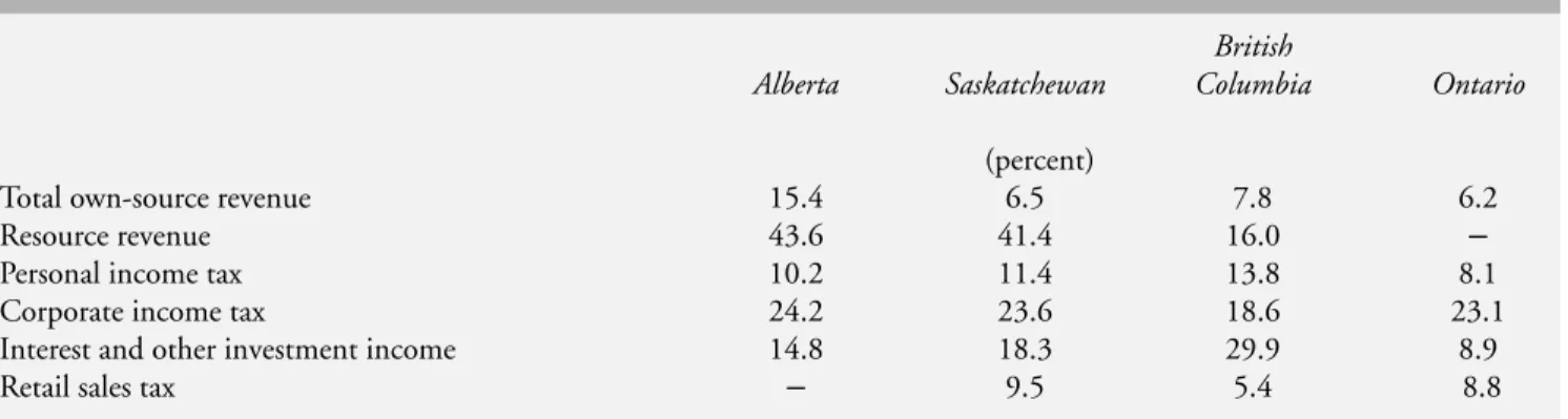
Table 7: Coefficients of Variation for Various Revenue Types, Selected Provinces, 1981-2007
Note: The coefficient of variation, a measure of volatility, is the ratio (multiplied by 100) of the standard deviation of the differences from an exponential trend to the average value of the series. Values for Alberta's retail sales tax and Ontario's resource revenue are not included because Alberta does not have a general retail sales tax that is comparable to the retail sales taxes in the other provinces, and Ontario's resource tax royalties are extremely small.
Source: Authors’ calculations using Statistics Canada data; see the Data Appendix for more information.
British
Alberta Saskatchewan Columbia Ontario
(percent)
Total own-source revenue 15.4 6.5 7.8 6.2
Resource revenue 43.6 41.4 16.0 –
Personal income tax 10.2 11.4 13.8 8.1
Corporate income tax 24.2 23.6 18.6 23.1
Interest and other investment income 14.8 18.3 29.9 8.9
other provinces: the coefficient of variation for real per capita sales tax revenue is only 5.4 for British Columbia and approximately 9 for both Saskatchewan and Ontario (Table 7).
A simple example illustrates the potential impact on Alberta’s revenue volatility of greater reliance on a sales tax.11This example is intended to give a general indication of the effect of the adoption of a sales tax on overall revenue
volatility, not to act as a policy prescription. While it is possible to estimate the tax revenues Alberta could have raised from a sales tax, we use the
more straightforward procedure of assuming that Alberta could have collected real per capita sales tax revenues equal to those levied by British Columbia during the 1981-2007 period.12 Rather than add a sales tax to the existing revenue base and, therefore, increase the total tax burden, we assess the impact on volatility of substituting the sales tax revenues raised by British Columbia for the revenues raised by the Alberta corporate tax. We chose the corporate tax because it yields volatile revenues that, on average, are similar in magnitude to the revenues raised from the British
11 This example differs from the proposal in McKenzie (2000) to replace Alberta's personal income tax with a sales tax, which is unlikely to have a significant impact on revenue variation since both personal income tax revenues and sales tax revenues are quite stable (see Table 7). 12 To make the level of revenues similar in the two cases, we use British Columbia's actual real per capita retail sales tax revenues to replace Alberta's
alcohol and tobacco tax revenues as well as its corporate tax revenues. With these changes, Alberta's real per capita own-source revenues would have averaged $7,419 over the period, as opposed to the actual value of $7,105. If Alberta were to introduce a sales tax, it would probably be in the form of a value-added tax rather than a typical retail sales tax. However, the available data are for a retail sales tax only, so our simulations employ these data.
-2000 -1500 -1000 -500 0 500 1000 1500 2000 2500 1981 1982 1983 1984 1985 1986 1987 1988 1989 1990 1991 1992 1993 1994 1995 1996 1997 1998 1999 2000 2001 2002 2003 2004 2005 2006 2007
Alberta Saskatchewan BC Ontario
Note: Values are in constant 2002 dollars.
Source: Authors’ calculations using Statistics Canada data; see the Data Appendix for more information.
Figure 3: Real Per Capita Own-Source Revenue minus Royalties, Difference from Trend, Selected Provinces, 1981-2007
Columbia sales tax. Holding everything else constant, the adoption of a sales tax yielding per capita revenues identical to those collected by British Columbia, along with the elimination of the volatile corporate profits tax, would cause the volatility of Alberta’s own-source revenues to fall by only 11.5 percent (from 15.4 to 13.6). Thus, even the complete replacement of volatile corporate tax revenues with much more stable sales tax revenues would yield only a relatively small drop in the volatility of own-source revenues. The reason for this small change in volatility is that sales tax revenues are fairly small compared with resource revenues and, thus, the volatility of revenues would continue to be driven by resource revenue volatility.13
Other Sources of Revenue
The opportunity to reduce revenue volatility by exploiting revenue sources other than the sales tax also appears limited. Personal income tax revenues tend to be relatively stable and are only weakly correlated with resource revenues and energy prices (Tables 2 and 6). On the other hand, in 2007, real per capita personal income tax revenues were already higher in Alberta than in British Columbia and Saskatchewan, although lower than in Ontario, and a similar comparison holds, on average, for the whole period from 1981 to 2007 (Figure 2). Thus, there might be little room to increase revenues from this source by enough to reduce overall revenue volatility, particularly without significantly increasing the level of tax-induced distortions.
Some of the smaller provincial tax bases are quite stable. For example, gasoline taxes have a coefficient of variation of only 3.2 over the period from 1994 to 2007, while the coefficient of variation for gambling revenues is 6.3. Payroll taxes have been a stable source of revenues in Ontario, with a coefficient of variation of only 2.1 over the period from 1992 to 2007,14and health care premiums were a stable source of revenues for Alberta. Nevertheless, greater use of these taxes to reduce overall revenue volatility would have only a minor impact; in some cases, greater use of these taxes might even have undesirable consequences. Alberta already exploits gambling revenues to a greater extent than do the other provinces, so it is unclear whether there is much opportunity for further diversification into this tax base.15There may also be little room for further expansion of alcohol and tobacco taxes, while greater reliance on property tax revenues could crowd out local government tax revenues. The introduction of a payroll tax (as used by Ontario) might raise the cost of labour and, potentially, have a negative impact on employment and other tax revenues. Finally, given the large share of resource revenues in total revenues and the magnitude of resource revenue volatility, none of the prospective tax bases is large enough or has enough room for further expansion to have an appreciable effect on overall revenue volatility.
In summary, tax base diversification likely would have a relatively minor effect on Alberta’s revenue volatility because its resource revenues are large and volatile relative to the alternatives. Tax base diversification could reduce revenue volatility
13 If, alternatively, we add British Columbia's sales tax revenues to Alberta's total own-source revenues less alcohol and tobacco taxes, leaving resource and corporate tax revenues unchanged, the coefficient of variation falls to only 13.8, while the total own-source tax burden rises by 13 percent. A further alternative is to use a sales tax to replace the proportion of resource revenues that is, on average over the 1981-2007 period, of equal magnitude to the revenues from the sales tax. In this case, the coefficient of variation in Alberta falls to 9.4, a level that is only about 40 percent greater than the average volatility in British Columbia, Saskatchewan, and Ontario. The larger decline in own-source revenue volatility in this case results because revenues from the most volatile revenue type –resource revenues –are cut almost in half. This would represent a large fall in the size of the payment for the resource and, thus, a large transfer from the residents of Alberta to the owners of resource firms. Further, to the extent that resource revenues arise from taxes on rents, the replacement of these revenues with revenues from another tax might not be efficient.
14 Ontario collects approximately $300 per capita in payroll taxes, measured in constant 2002 dollars.
15 In 2007, measured in per capita 2002 dollars, Alberta collected $434 in gaming profits, while British Columbia, Saskatchewan, and Ontario collected $223, $280, and $105, respectively.
only if the revenues collected from the unstable energy and corporate tax bases were significantly reduced as a proportion of total revenues. This would entail a significant increase in taxes from other sources and, thus, in the overall tax burden, or a significant decrease in the revenues collected from resources and corporate taxes.
Revenue Volatility and Stabilization from Exchange Rate Movements
Movements in the Canadian dollar tend to reduce the volatility of movements in Alberta government resource revenues. This occurs because there is a generally positive relationship between the value of the Canadian dollar and the US dollar prices of oil and natural gas (Bayoumi and Mühleisen 2006).16For example, a rise in the US dollar price of oil raises the US dollar value of oil revenues. However, since the Canadian dollar appreciates with the increase in the US-dollar-denominated oil price, there is less of an increase in the Canadian dollar value of resource revenues. Similarly, a fall in the US dollar oil price leads to a depreciation of the Canadian dollar, causing a smaller decline in the Canadian dollar value of oil revenues. In this way, the exchange rate acts as a “natural hedge” that cushions oil price movements (Frankel 2005).
Canada’s exchange rate policy is beyond the control of the Alberta government. However, the Bank of Canada’s policy of inflation targeting is likely to increase the smoothing effect of exchange rate movements on the Canadian dollar value of energy revenues. Ragan (2005) argues that, to reduce inflationary pressure following a
commodity price rise, the central bank tightens monetary policy, which leads to an appreciation of the Canadian dollar. In this way, inflation targeting tends to accentuate the positive oil price-Canadian dollar correlation, thus increasing the
smoothing effect of exchange rate movements on Canadian-dollar-denominated energy revenues.
The exchange rate moves for many reasons other than changes in energy prices, so
movements in the exchange rate only partly offset movements in US-dollar-denominated energy prices. Thus, while exchange rate movements have reduced Canadian dollar oil and gas price volatility, the volatility of both commodity prices in Canadian dollars remains high. Measured over the period from 1981 to 2007, the volatility of the real price of oil in Canadian dollars was 16 percent smaller than the volatility in US dollars, while the volatility of natural gas was 9 percent smaller, but the coefficients of variation of the prices of both commodities in Canadian dollars are still quite large, at 39.4 for oil and 42.0 for natural gas (Table 2).
Smoothing with Futures Options
Revenue volatility and uncertainty can be reduced with financial instruments specifically designed for this purpose. For example, it is possible to pre-sell commodities at a known price in futures markets or to purchase “put options” –contracts that give the purchaser the option, but not the obligation, to sell a commodity at a stated price for a fixed period of time.17
Futures Market
In Alberta, conventional crude oil royalties are paid in-kind (Alberta 2008, 7). If these in-kind royalties are sold in the spot market as they are received, the revenue stream associated with the royalties will depend on the uncertain and volatile path of oil prices. An alternative to selling in-kind royalties on the spot market is to pre-sell these royalties, at some time prior to receipt, in the futures market. This would eliminate uncertainty with respect to the revenues received from the 16 A similar positive co-variation between currencies and the price of export commodities is found for other countries, including Australia,
New Zealand, Chile, and South Africa (Chen and Rogoff 2003; Cashin, Céspedes, and Sahay 2004). This co-variation is consistent with a rise in the world demand for a commodity that then causes a rise in demand for the currencies of the countries that export the commodity. 17 The use of such "hedging" strategies by Alberta is raised as a possibility in Tuer (2002, 66). See also Fildes, Koziol, and Riddell (1993); and
royalty payments since the price would be fixed by the futures contract. Further, futures prices, at least for contracts that are sold 12 months or more in advance, have been found to be less volatile than spot prices (Daniel 2001; Domanski and Heath 2007), so pre-selling in futures markets also might reduce volatility.
While futures markets can reduce revenue uncertainty and volatility, several potential shortcomings are associated with their use. First, the majority of transactions in futures markets involve relatively short-term contracts (one or two months), but to have a significant impact on uncertainty and revenue volatility, the government would need to enter into futures contracts that cover at least the current budget year. As futures markets are not generally very liquid at longer maturities, the sale of the longer-term contracts needed to reduce volatility is likely to be more costly (see Larson, Varangis, and Yabuki 1998; Domanski and Heath 2007; Borensztein, Jeanne, and Sandri 2009). Second, futures contracts cannot eliminate all revenue volatility since new contracts will be sold through time and the price locked in by these contracts will vary with changes in the futures price. Third, while the direct
transaction costs of futures contracts are relatively small, these contracts generally require the
commitment of significant assets to cover margin payments, and the magnitude of these payments can change by a large amount at short notice with changes in the price of the underlying
commodity.18Finally, it is practical to use futures contracts only to reduce the volatility of royalties received in-kind,19but such royalties form a relatively small part of total resource revenues –
conventional oil accounted for only 12.8 percent of total non-renewable resource revenues during
the 2005-09 period, or about 4 percent of total own-source revenues (Table 5).20
Options Market
The purchase of put options is an alternative method of reducing revenue uncertainty and volatility. Put option contracts provide insurance against price declines by giving the purchaser of the contract the option, but not the obligation, to sell a commodity at a price fixed by the contract –
the “strike” price –if the market price falls below this price. The purchase of options contracts has two key advantages over futures contracts. First, while a futures contract removes the downside risk of a price decline by fixing the future price, it also eliminates the potential benefit from a price rise. The purchase of an options contract, on the other hand, lets the purchaser benefit from price rises, but protects against a price fall. Second, options contracts, unlike futures contracts, do not restrict hedging to in-kind royalty payments only. For example, Alberta could insure itself against a resource revenue decline by purchasing options; then, if the market price of oil fell below the price specified in the option, the government would earn the difference between this price and the market price. These profits would counterbalance any fall in the value of royalties, both cash and in-kind, associated with the fall in the market price of oil.
A number of oil-exporting jurisdictions –
Ecuador, Mexico, and Texas, for example –have used option contracts to hedge against price declines. Nevertheless, despite the potential benefits of hedging with options contracts, it is not common for energy-exporting countries to hedge (see Blas 2009; Borensztein, Jeanne, and Sandri 2009). Alaska, New Mexico, Oklahoma, 18 Daniel (2001) suggests that margin payments can amount to 5 to 10 percent of the value of the contract.
19 While it is possible to hedge royalty payments other than those paid in-kind using futures contracts, this could expose the province to a potentially large liability. For example, suppose Alberta were to sell a greater number of petroleum futures contracts than the quantity of its in-kind royalty payments and the price of petroleum rose relative to the price stipulated in the futures contracts. The province would then be responsible for making up the difference between the spot price and the contracted futures price without necessarily having a counterbalancing rise in its own revenues, since energy prices and royalty revenues, although highly correlated, do not necessarily move one for one.
20 Hotz and Unterschultz (2009) use simulations to assess the benefit of using futures markets to reduce budget forecast errors. Using data from the 1995-2004 period, they conclude that the benefits for Alberta are unlikely to outweigh the costs.
and Louisiana have all examined the costs and benefits of options and decided not to proceed in this direction.
One reason jurisdictions might have hesitated to use options markets to reduce the volatility of revenues is political (see Daniel 2001; Caballero and Cowan 2007; Frankel 2010). If the market price remains above the strike price for the duration of the contract, the jurisdiction that purchased the put option does not reap an explicit benefit, but still bears the cost of purchasing the option. While this is a characteristic of every insurance contract, a government might find it difficult to explain to the public why it committed significant resources to the purchase of options contracts that were worthless ex post (Caballero and Cowan 2007). This type of outcome has been used to accuse governments of using public money to “speculate” in commodity markets –
in Ecuador, for example, it led to allegations of corruption (Daniel 2001). In contrast, if the government does not hedge, it can blame any budgetary problems on the vagaries of the international oil market or speculators.
Another problem with the use of put options to insure against a revenue fall is that these options are generally expensive. Mexico’s 2010 hedge of 230 million barrels of oil cost US$1.2 billion, a little over US$5 per barrel. Alaska (2002)
estimates that a three-year put option with a strike price US$1 below the three-year futures price would have cost US$3 per barrel, or 11 percent of the spot price at the time (US$26). Simulations for the case of Texas show that the ex post net insurance premium associated with the use of options was equal, on average, to 2.6 percent of oil revenues (Swidler, Buttimer, and Shaw 1999). Thus, the cost of hedging can amount to a significant proportion of total revenues.
Several other potential shortcomings are associated with the use of options as a method of smoothing revenues, most of which are similar to the shortcomings of futures contracts. First, put options insure against a fall in prices only during
the length of the contract, but since contract lengths are not indefinite, full insurance cannot be obtained. Second, the purchase of longer-term contracts is likely to be more expensive, as most of the liquidity in the options market is at very short horizons. Borensztein, Jeanne, and Sandri (2009) note that most hedging through NYMEX is for maturities of less than three months’ duration and that the risk premium becomes very large for longer maturities. It is possible to buy longer-term options in the over-the-counter market, but these contracts are illiquid and involve greater
counterparty risk than options traded on an exchange. Third, a government that follows a hedging program, particularly one using over-the-counter instruments, must possess sufficient expertise to run the program, understand the risks, and monitor the activities of the hedging unit in order to protect against trading losses.21 Finally, while options can eliminate downside price risk, options do not reduce revenue volatility on the upside, and the reduction in downside risk may even encourage excessive spending when prices are high.
Revenue Volatility with a Stabilization Fund The analysis above makes clear that revenue volatility in Alberta is driven by resource revenue volatility. On average, over the period from 1981 to 2007, the volatility of real per capita own-source revenues excluding reown-source revenues has been similar in Alberta, Saskatchewan, British Columbia, and Ontario; accordingly, stabilization of the revenue from resources is the key to
stabilizing Alberta government revenues. An effective method to achieve revenue
stabilization would be through the establishment of a resource revenue stabilization fund. While Alberta has the Alberta Heritage Savings Trust Fund (AHSTF), the objective of this fund is not the reduction of revenue volatility per se. In a report commissioned by the Alberta Minister of Finance, Tuer (2002) proposes that the AHSTF be 21 As Larson and Varangis (1996, 28) note, the "cases of Codelco (a copper producer in Chile), MG Corp. (a unit of Germany's
Metallgesellschaft AG), Procter and Gamble Co., Orange County in California, Sumitomo, and Barings Bank have shown that the lack of internal controls and systems to monitor the exposure from using derivative markets can result in very serious losses."
redesigned to stabilize the impact of volatile resource revenues on the province’s budget, but this has not been done. There is also the Alberta Sustainability Fund, created in 2003 and designed to stabilize revenues but it, along with the AHSTF, has been subject to considerable discretion in terms of
contributions and withdrawals (Busby 2008). Key Features of a Stabilization Fund
The two key design elements of the stabilization fund we propose are the commitment of a fixed percentage of volatile current resource revenues to the fund, and the withdrawal –the transfer to current government revenues –of the long-term real earnings of the fund and a fixed percentage of the total assets in the fund.22A fund with these characteristics would reduce volatility in three ways. First, a proportion of the most volatile component of revenues, resource revenues, would be deposited in the fund and, therefore, excluded from current government revenues. This would leave the more stable components of revenues, plus withdrawals from the fund, available for current spending. The ability of the fund to reduce volatility would be greater the larger were the share of resource revenues deposited in it.23
Second, fund withdrawals would be based on a long-term average real interest rate. An average would reduce the volatility of this component of transfers to government revenues, since returns
vary considerably from year to year. In general, the longer the averaging period, the smaller would be the volatility of real returns.
Third, withdrawals each year would be a constant fraction of the fund’s stock of assets. This would reduce revenue volatility because the revenue paid out by the fund in a particular year would be based on an unchanging fraction of contributions from all previous years.24A withdrawal formula of this type also would effectively eliminate the possibility of zero
transfers from the fund during a year –in contrast to the experience of the AHSTF, where no
transfers to general revenues were made in fiscal years 2002/03 and 2008/09, when the value of the fund declined.25
The stabilization fund we describe here would not be a “rainy day” fund, as extra funds would not be withdrawn when there was a negative disturbance to revenues. Rather, the fund would smooth revenues by weakening the link between current resource revenues and current budgetary revenues. Further, the proposed fund would not require the government to identify the conditions under which contributions and withdrawals should be made. An added benefit of fixed contribution and withdrawal rates is that they likely would limit discretion, which can contribute to revenue volatility. As well, this type of fund would be transparent and easy to understand.26
22 One way to make the fund even simpler and easier to understand, with little impact on the degree of stabilization, would be to dispense with the withdrawal of real earnings and raise the fixed percentage of total assets withdrawn each year.
23 Fixed savings-fund contribution rates are used by both Alaska (25 percent) and Norway (100 percent).
24 It is typical for stabilization funds to incorporate discretionary withdrawals (Davis et al. 2003, 282-3). Some funds rely on price forecasts or moving averages of prices to determine contributions and withdrawals, but energy price forecasts are often inaccurate (Ossowski et al. 2008, 6) and, given the persistence of energy price movements, a moving average might give too much weight to recent prices. Even when spending depends on a five-year moving average of resource revenues, a spike in resource prices can cause a large spike in expenditures (Kneebone 2006b, 7).
25 With the current design of the AHSTF, revenue payouts into general revenues from the fund are equal to all current income of the fund, less an amount required for inflation proofing (Alberta 2010a, 5).
26 Another budgeting method that has been used to reduce the risk of a revenue shortfall and the need to cut expenditures is to underestimate revenues. Tying expenditures to a downward-biased revenue forecast would not change the degree of revenue volatility, but would provide a buffer against an unexpected fall in revenue. This type of policy could also be used as a backdoor method of creating a “rainy day” fund, if the “unexpected” surpluses were saved, but it likely would be difficult to create a sizeable fund in this way. A policy of this type also has two other shortcomings. First, the ex post budget surpluses that result on average could be easily identified and might induce demands for increased spending; for example, at the federal level, Robson (2006) argues that “padding” the bottom line in budget projections has led to extra fiscal room and spending hikes. Second, this type of policy would quickly make budget forecasts non-credible and could lead to a political backlash and calls for tax reductions, which would defeat the purpose of the buffer.
A related benefit of this type of stabilization fund is that it would reduce revenue uncertainty, as current and future revenues would depend on past contributions and the long-term earnings of the fund. As a result, the government would have considerable information on the future path of transfers from the fund and could use this
information to plan expenditures, which, in turn, might encourage the province to take a longer term view of budgeting. An added advantage is that, since the fund would be backward-looking, forecasts of future energy prices, which tend to be highly uncertain, would not be required. In particular, the government need not estimate whether a shock to energy prices was transitory or permanent.
While such a stabilization fund is designed to address revenue volatility, it would also create a store of wealth for future generations, which makes it similar to a savings fund. Proponents of savings funds take the view that, since resource revenues arise from the conversion of physical assets into financial assets, governments should treat resource revenues as wealth and, therefore, should spend only the annuity value of this wealth, leaving the balance in a savings fund to support the provision of services to future generations.27The fund we propose here would differ, however, from a pure savings fund in terms of the payout rule, which, in general, would be greater than the real rate of interest. Nevertheless, as the stabilization fund smooths revenues over long periods, it likely would transfer resources between generations.28
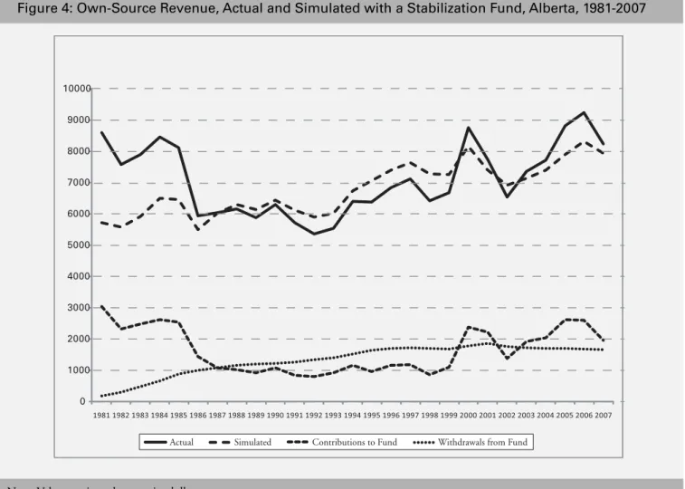
An Example of Revenue Stabilization with a Fund
Using data on actual revenues over the past 30 years, a simple example shows the extent to which a stabilization fund could reduce revenue
volatility.29In this simulation, 75 percent of Alberta’s resource revenues are committed to a fund each year; if all non-renewable resource revenues were added to the fund, as Tuer (2002, 51) recommends, there would be even greater revenue stabilization.30Each year, the fund pays out to general revenues the average real earnings of the fund plus 5 percent of the total assets in the fund. Since real interest rates vary considerably, greater smoothing is achieved with the use of an average return over a long period, so the
simulation employs the average medium term real Government of Canada bond yield over the previous 20 years. Five percent, or one-twentieth, of total assets is withdrawn each year in order to smooth earnings over many years.31A long time frame assists in revenue smoothing since Alberta revenue downturns and upturns tend to be long lived, often lasting five to ten years, as we showed in Figure 1.32
Under this scheme, the volatility of own-source revenues, net of contributions to and withdrawals from the fund, falls from 15.4 to 5.9, a decline of over 60 percent. This level of volatility is lower than the revenue volatility of British Columbia, Saskatchewan, and Ontario (Table 7). Figure 4 illustrates the simulated contributions to the fund and withdrawals from the fund as well as the
27 Studies that discuss savings funds and the related issues of intergenerational equity and fiscal sustainability include Engel and Valdes (2000); Barnett and Ossowski (2002); Davis et al. (2003); Kneebone, McKenzie, and Taylor (2004); and Mintz (2007).
28 In the extreme case in which payments into the stabilization fund ceased, payments out of the fund also would eventually end. For the example presented below, however, if payments into the fund stopped completely, it would take approximately 14 years for the value of the fund to fall by half.
29 This example is intended for the purposes of illustration and does not adjust for the actual savings of the Alberta government during the sample period, such as saving through the AHSTF and other provincial government funds.
30 When the AHSTF was established in 1976, it received only 30 percent of non-renewable resource revenues. The contribution rate was later reduced to 15 percent and then in 1987 to zero. The government chose to deposit over $1 billion in the AHSTF from general revenues in each of fiscal years 2005/06, 2006/07, and 2007/08, part of which was allocated for inflation-proofing (Alberta 2010b).
31 The average real return is 3.4 percent, so withdrawals from the fund average 8.4 percent per year.
32 Tuer (2002, 52) recommends that the amount withdrawn should be the lesser of the average of resource revenues for the previous three years, or $3.5 billion (the 20-year average of resource revenues). Given the large and often long-lived swings in resource revenues, Tuer's proposed rule, based as it is on revenues from just the previous three years, likely would lead to greater volatility than the 5 percent rule we propose.
actual and simulated levels of own-source
revenues. The smoothing effect of the fund is clear from a comparison of the smooth path of
withdrawals with the volatile path of contributions.33
Implementation and Other Issues
The experiences of Alberta and other jurisdictions reveal that a fiscal rule alone, such as the creation of a stabilization fund, cannot ensure compliance (see O’Brien 2010; Ossowski et al. 2008). Key characteristics of a stabilization fund that may increase the probability of success are simplicity,
transparency, and a gradual transition to full implementation.
The establishment of a stabilization fund would require a start-up period in which contributions to the fund initially exceeded withdrawals. To avoid a sharp rise in taxes or fall in current expenditures during this period, the contribution rate could be gradually increased to the target level. Since it would lower the required maximum net savings rate out of resource revenues, a contribution rate transition period could increase the likelihood that policymakers adhere to the fixed contribution and 0 1000 2000 3000 4000 5000 6000 7000 8000 9000 10000 1981 1982 1983 1984 1985 1986 1987 1988 1989 1990 1991 1992 1993 1994 1995 1996 1997 1998 1999 2000 2001 2002 2003 2004 2005 2006 2007
Actual Simulated Contributions to Fund Withdrawals from Fund
Note: Values are in real per capita dollars.
Source: Authors’ calculations using Statistics Canada data; see the Data Appendix for more information.
Figure 4: Own-Source Revenue, Actual and Simulated with a Stabilization Fund, Alberta, 1981-2007
33 Average per capita own-source revenues available to the government, net of contributions to and withdrawals from the stabilization fund, would have been only 4.5 percent lower than actual average real per capita own-source revenues for the period from 1981 to 2007. This lower average level of revenues follows because, in the initial years, the government makes contributions to the fund, but the fund has few assets to disburse. Real per capita own-source revenues, net of contributions to and withdrawals from the fund, would have still been 25 percent higher than the average for Saskatchewan, British Columbia, and Ontario. In addition, the total assets in the fund would have been close to $75 billion by 2007. Thus, this fund, in combination with the Alberta government's other funds, would have yielded a stock of assets similar in size to the $100 billion savings fund proposed by Mintz (2007).
withdrawal rules.34Meeting targets would be particularly important in the fund’s early years, as this would generate credibility with the public.35 Of course, the longer the transition period, the longer it would take to attain the full volatility-reducing benefit of the stabilization fund.
Mintz (2007, 26) states that Alberta saved 30 percent of resource revenues between 1993 and 2007, while Kneebone (2006a) provides evidence that the province saved almost 50 percent of resource revenues between 1995 and 2005. Simulations, illustrated in Figure 5, indicate that the creation of a stabilization fund with a gradual
transition to the maximum contribution rate would require net savings rates that are generally below these levels. These simulations assume a fixed withdrawal rate of 10 percent, real earnings on the assets in the fund of 2 percent, and, for simplicity, a constant stream of resource revenues. If the stabilization fund were established with a transition period during which the contribution rate was gradually increased to 75 percent in annual increments of 15 percentage points, the net savings rate would exceed 50 percent in only one year (the fifth). Alternatively, if the
contribution rate were gradually increased in 34 Norway eased the transition when establishing its savings fund by not commencing contributions to the fund until the government's
budget was in surplus.
35 Kneebone (2006b) argues that the pre-announced and feasible deficit targets introduced by Alberta in the 1990s helped build credibility for the deficit reduction plan, which contributed to its success.
-20 -10 0 10 20 30 40 50 60 70 1 2 3 4 5 6 7 8 9 10 11 12 13 14 15 16 17 18 19 20 21 22 23 24 25 26 27 28 29 30 31 32 33 34 35 36 37 38 39 40
Immediately to 75 To 75 in increments of 5 To 75 in increments of 15
Note: Transition to a 75 percent deposit rate with constant resources revenue, a 10 percent withdrawal rate, and a 2 percent yield on assets Source: Authors’ calculations.
increments of 5 percentage points to 75 percent, the net savings rate out of resource revenues would exceed 30 percent during four years, although only by a small percentage.36
While shocks to resource revenues could put pressure on the budget and lead to calls for the fixed deposit and withdrawal rates to be abandoned, this would be largely a transition issue. Once the stabilization fund was fully in place, the budget would be insulated from
resource shocks as volatile revenues were deposited in the fund and an average of all previous
contributions withdrawn. Even large movements in non-renewable resource revenues would have a relatively minor impact on revenues net of contributions and withdrawals from the fund.37
One drawback of such a fund is that, as the fund grows in size, pressure might mount for taxes to be cut or the proportion of assets withdrawn from the fund to be increased, making it difficult to maintain contributions to the fund and prevent ad hoc withdrawals. A purpose of simple,
transparent, and fixed contribution and withdrawal rules would be to counter this tendency by making changes to the operation of the fund obvious and easily understood. Frankel (2010, 30-1) stresses the importance of a rule that dictates a cap on spending out of a fund “to insure that politicians will not raid the fund when it is flush.” However, even if the government maintained fixed contribution and withdrawal rates, it could circumvent the fund by financing expenditures through debt accumulation. Ossowski et al. (2008, 24) suggest that “greater focus on the non-oil balance in budget
documents…may foster an informed debate of fiscal policy choices.”38Thus, if budget papers treated government revenues as net of
contributions to and withdrawals from the
stabilization fund, deficits would be transparent to both the public and policymakers.
Former deputy treasurer of Alberta Al O’Brien (2010) notes that a key lesson from the “Klein revolution” during the 1990s is that, to be successful, a policy must enjoy the understanding and support of the public and key stakeholders. Further, he argues that the policy must be
characterized by simple and open communication, as well as clear targets, accompanied by the
meaningful measurement of results. Unlike savings funds, which are focused on the more distant goals of intergenerational equity and fiscal sustainability, a stabilization fund would have a short-term goal: the stabilization of revenues to support stable expenditures.
As many Albertans have experienced the real costs associated with boom-and-bust spending paths, it might be easier to build public support for a stabilization fund. In contrast to Alberta’s Sustainability Fund, which has complex rules for contributions and withdrawals that have been changed frequently, the stabilization fund we propose would be simple, transparent, and straightforward, which would make it easy to understand, communicate, monitor, and evaluate. Given Alberta’s fiscal history, these features likely would be critical to the success of such a fund.
Conclusion
Volatile revenues can lead to the inefficient provision of government services, stop-go
procyclical fiscal policies, and, potentially, slower growth. Alberta’s government revenues are volatile relative to those of other provinces, a volatility associated principally with that of energy sector revenues. Indeed, Alberta’s own-source revenues less resource revenues are no more volatile than the corresponding revenues of other provinces. One problem with revenue volatility is that it usually leads to volatile government expenditures. Revenue volatility is likely to be less of a problem
36 If the contribution rate out of resource revenues is set to 75 percent immediately upon establishment of the fund, net savings out of resource revenues would be 67.5 percent in the first year, but the savings rate would fall below 50 percent by the fourth year and below 25 percent in year ten.
37 Norway's contribution rate of 100 percent effectively insulates its budget from oil price shocks (Ossowski et al. 2008). 38 This is also consistent with the recommendations in Barnett and Ossowski (2002).