Evidence from Germany

Estimating Dynamic Income Responses to Tax Changes

Evidence from Germany

Nima Massarrat-Mashhadi

Clive Werdt

School of Business & Economics

Discussion Paper

FACTS

Estimating Dynamic Income Responses to Tax Changes:

Evidence from Germany

Nima Massarrat-Mashhadi1

Department of Finance, Accounting and Taxation, Freie Universität Berlin

Clive Werdt

Institute for Public Finance and Social Policy, Freie Universität Berlin

December 13, 2012

Abstract

This paper provides new empirical insights on the elasticity of taxable income to the net-of- tax rate. Using a panel of German income tax return data, we followed taxpayers from 2001 to 2006 to analyze the effects of the German tax reforms of 2004 and 2005. Implementing a dynamic model as proposed by Holmlund and Söderström (2011), we are able to disentangle short-term and long-term responsiveness. These estimates allow us to distinguish between different dimensions of behavioral changes: short-term income reactions in contrast to ‘real’ changes in (reporting) behavior. We compare our results with recent German estimates from the established approach by Gruber and Saez (2002) applied by Gottfried and Witzcak (2009). Following Chetty`s (2009) theoretical considerations, we use multiple (tax code related) income concepts and alternative sample choices. We provide several robustness and validity analyses of the most common income concept, i.e. taxable income excluding capital. Our preferred specification yields (very) high short-term yet small long-term elasticites. The latter range from 0 to 0.16, implying none or only modest persistent behavioral changes to marginal tax rate cuts.

Keywords: Long-term income responses, taxable income elasticity, dynamic panel data estimation, income tax return data

JEL codes: C26, H21, H53

1_{Author of correspondence: Department of Finance, Accounting and Taxation, Free University Berlin,}

Garystraße 21, 14195 Berlin, Germany. E-mail: [email protected]. We are grateful to Timm Bönke, Giacomo Corneo, Frank Fossen, Bertil Holmlund, Jochen Hundsdoerfer and Victor Steiner for valuable discussions. Earlier drafts were presented at the Wirtschaftspolitisches Seminar at the Free University Berlin. We would like to thank all participants for their comments. The usual disclaimer applies.

1 Introduction

For the evaluation of tax reforms the elasticity of taxable income to net-of-tax rate (ETI) has emerged as the central fiscal policy parameter (Feldstein 1995, 1999) over the last years. It is defined as the percentage change in taxable income that results from a percentage change in the net-of-tax rate (NTR). ETI has been established to capture more dimensions of behavioral responses to income tax reforms than labor supply elasticity estimates.

Since Feldsteins’ (1995) seminal contribution, a massive body of ETI literature has emerged. A very comprehensive overview of empirical results and econometric methodology is provided by Saez et al. (2012). The review can be further considered a guideline for proper research on ETI. The authors survey the most common estimation strategies; discuss possible drawbacks and identification issues. They highlight that dynamic panel estimation strategy is a promising complement and improvement of estimation methodology for future research. The majority of previous empirical results on ETI have focused on immediate income responses to tax changes, based on a prominent specification by Gruber and Saez (2002). Most US studies suggest an ETI within a range of 0.3 and 0.6.2 German findings tend towards a similar size.

Gottfried and Witczak (2009) were first to adopt Gruber and Saez’ approach using German income tax return data. Their preferred specification reports an elasticity of taxable income of 0.6. Empirical findings for Germany and Europe are still scarce.3 Relying on the dynamic approach by Holmlund and Söderström (2011), we do not only contribute to the literature by delivering further ETI estimates: (1) We distinguish between immediate and persistent behavioral changes, resulting from the tax reforms. (2) By applying alternative income concepts and different sample choices, we provide a wide range of ETI estimates and test their sensitivity. We analyze the German tax reforms of 2004 and 2005 and use the most recent and very rich German income tax return data (assessment years 2001 to 2006). This major reform is characterized by both tax base broadening and a reduction of all marginal tax rates. Our approach differs in several aspects from the prevalent approach in the literature: (1) Our data allow us to observe not only cuts in tax rates for some taxable incomes, but for the

2 _{Auten and Carroll (1999) & Gruber and Saez (2002) provide important estimates for US tax reforms.}

3 _{Two other studies exist for the German case. Gottfried and Schellhorn (2004) analyse the 1990 change in}

personal income tax schedule for taxpayers in Baden-Wuertemberg. Their results suggest an average ETI of 0.4. Controlling for business income and high-income households, they find values up to 1.0. Müller and Schmidt (2012) contribute in German language by their analysis of the German income tax reforms of 2004 and 2005. Relying on the common approach by Gruber and Saez (2002), they find small elasticities, ranging from 0.2 to 0.4.

whole distribution of taxable income. (2) Contrary to other tax schedules, the German Income Tax Code assigns varying marginal tax rates between and within brackets as taxable income rises. (3) Behavioral responses to marginal tax rate changes are likely to be not only immediate but rather gradual; we pioneer with providing short- and long-term estimates of taxable income elasticity for Germany. Providing separate estimates for single and married taxpayers, we also control for immense differences in tax planning potential between married and single taxpayers. Moreover, married taxpayers benefit from a splitting boon, which heavily discriminates between these two groups. Single taxpayers differ in various socio economic aspects from married taxpayers, implying different utility functions. In the regressions we use only taxpayers which do not change from single filing to joint taxation. This causes a possible selection bias for sample with the single taxpayers. This is a fairly long time given that our sample comprises mainly of middle aged income earners.

These differences are likely to be non-linear and hard to control for properly in (linear) regressions. Regression results approve the empirical need for the separation. Results are drawn from a balanced panel of income data, using years 2001 to 2005. We do not only find substantial differences in responses between single and married taxpayers but also between income concepts, pointing to a cautious and thorough evaluation of the German income tax reform. Controlling for the influence of taxpayers at the top end of the income distribution, we find that estimates are (very) sensitive to sample selection and observation periods. Our empirical findings indicate that long-term behavioral changes are considerably smaller than short-term reactions, while single taxpayers tend to be less short-term responsive than married taxpayers. Relying on our preferred specification, the latter show a significant and pretty robust short-term reaction, amounting to 1.07 with a considerably small long-term reaction of 0.14. For single taxpayers, the short-term elasticity of 0.62 is much lower and similar to the long-term responsiveness, amounting to 0.49. Using three alternative tax-code related income definitions, our robustness analysis enables us to interpret special tax responses from different income sources. While income from capital does not drive the elasticity estimates, income from rent & lease exhibits significant influence on long-term estimates. The general pattern shows a strong short-term reaction to the German income tax reform, exceeding unity for married taxpayers and 0.6 for single taxpayers. Long-term responsiveness are harder to identify precisely, ranging from -0.40 to 0.49.

Following Chetty’s (2009) objections on the validity of ETI for welfare analysis, we also estimate elastiticities based on an alternative income concept, relying mostly to the ideas of Bach et al. (2009). These findings suggest an unintuitive and strong(er) short-term and

long-term behavioral response for single taxpayers, accentuating the sensitivity of estimates, when “more realistic” income measure is derived.

The paper proceeds as follows. Section 2 gives a short overview of the German tax system and describes the German tax reforms. Section 3 presents the data and its preparation. The empirical strategy is discussed in Section 4. Section 5 presents our empirical findings and compares with recent German results. Section 6 concludes.

2 The German Income Tax System and Recent Reforms

The German income tax schedule is directly progressive, marginal tax liability increase with taxable income. Income above the basic tax allowance is divided into several brackets. Contrary to most other progressive tax systems, the German tax schedule is not a step system. The German tax schedule substantially discriminates between single and married taxpayers.4 Married taxpayers can opt for the splitting tax schedule to decrease their joint taxation and marginal tax rates.5

The change of government in Germany in 1998 was associated with intensive discussions about tax reforms. The new red-green government agreed upon several reforms of income and corporate taxation starting in 1999. It has been the biggest bundle of income tax reforms in Germany’s history since World War II. Prior to our observation period, two major parts of that reform bundle were implemented. One was a reform affecting personal income taxation indirectly.6 The other part of the reform was directly related to personal income taxation and aimed at reducing all marginal tax rates of the German tax schedule. Between 1999 and 2001 the bottom marginal tax rate was cut from 25.9% to 19.9%, whereas the top marginal tax rate was reduced by 4.5 percentage points from 53% to 48.5%. Marginal tax rates in-between were reduced accordingly. The most prominent tax reform was passed in 2000 and consisted of a further gradual reduction of personal income tax schedule, accompanied by modest tax

4 _{Steiner and Wrohlich (2007) provide their theoretical as wells as empirical evidence how different forms tax}

splitting affects economic dimension, e.g. household welfare and work incentives.

5 _{Marginal tax rates for married couples are determined as if one single taxpayer would earn the average}

taxpayers income. Accordingly, the tax burden is calculated as twice as much the single taxpayer with the average income would have to pay. Given the progressive schedule, married couples with uneven distributed incomes can reduce their overall tax burden, thus marginal tax rate. O´Donoghue and Sutherland (1999) discuss how joint taxation affects the incentives of the spouse of the main earner to earn income. They point out that “the earnings of one spouse [the secondary earner] may be taxed at a higher marginal rate than if they were single, or if they were the main earner. “

6 _{It was a significant paradigmatic change in corporate taxation, taking place between 2000 and 2001. Its main}

attribute was the reduction of the corporate tax rate from 45% to 25% combined with simultaneous corporate tax base broadening. The reform of corporate taxation also included several adjustments regarding the income taxation.

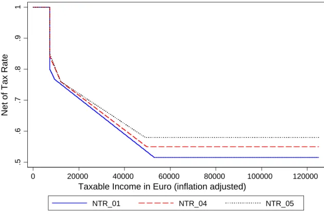
base broadening. It was implemented in our survey period from 2001 to 2005 and was by no means designed to be income tax revenue neutral but to foster economic growth.7 The reform combines several steps which lower the income tax schedule in 2001, 2004 and 2005. Besides the reduction of all marginal tax rates, the basic tax allowance was slightly increased from 7,206 EUR in 2001 to 7,664 EUR in 2005. Figure 1 depicts the NTR for single assessed tax units in 2001, 2004 and 2005 depending on taxable income. Since the tax base broadening had only little effect on the actual definition of taxable income, we are able to construct a time consistent taxable income. Estimation results are based on marginal tax rates from this income definition.8 .5 .6 .7 .8 .9 1

Net of Tax Rate

0 20000 40000 60000 80000 100000 120000

Taxable Income in Euro (inflation adjusted)

NTR_01 NTR_04 NTR_05

Fig 1. Net of Tax Rate for a single assessed tax unit in prices of 2005

7 _{Parallel to the income tax reform, the German government implemented another comprehensive set of labor}

markets reforms so called Hartz Reforms during our observation period between 2003 and 2005. These reforms fundamentally changed institutional and legal framework of the labor market and the benefit system. Merging unemployment assistance and social welfare transfers, restricting the rights of unemployed were cornerstones of the Hartz Reforms. Since the reduction of employment protection in some labor market segments is only a minor part of the Hartz Reforms, we do not expect significant interferences with the analysis and evaluation of the income tax reform.

8 _{We take the definition of taxable income in 2001 as our benchmark. We are able to control for the most}

important tax base broading measures: annual child allowances were modified from 2556 € to 2904 € per child, most loss offsetting rules were cancelled in 2004, allowable expenses for non-itemizing employees were reduced from 1044 € to 920 €, allowances for single parents were lowered from 2871 € to 1308 €, exemptions for capital gains of 1550 € were cut to 1370 €. Gruber and Saez (2002) point out that this procedure might underestimate the responsiveness of taxable income.

3 Data and data processing

Relevant information generated in the process of taxation is documented in the income tax return: information on the family situation, declaration of income from different sources, granted deductions and exemptions, calculation of taxable income, and personal income tax payment. The German Federal Statistical Office collects the official income tax returns electronically as Income Tax Statistics, providing the basis for a balanced panel, the German Taxpayer Panel. Individual taxpayer’s IDs are used to link annual cross section income tax returns over time to create the panel. However, this procedure might be problematic. In cases of marriage, divorce or moving to another federal state, individual tax ID will be given up, created new or changed. Additionally, German wage earners are not forced to file a tax return unless they have other sources of income. Moreover, the incentive for wage earners of filing a tax return depends on the expectation of a possible tax refund. The German Taxpayer Panel does not include tax returns, which are only available for a subset of years and not consistently linkable. It contains income tax returns of approximately 19 million observations out of possible 31 million taxpayers included in the Income Tax Statistics. Several socio-economic characteristics of taxpayers such as age, number of children, church membership and marital status are observable. On basis of four stratifications criteria, i.e. federal state, assessment type, main type of income and total income, a 5% sample is drawn and made available for scientific purposes. The stratification procedure aims to optimize the sample with regard to standard errors of total income over time. Observation weights are generated accordingly. For our analysis, we consider taxpayers who are fully liable to income tax, pay taxes and whose marital status does not change between 2001 and 2005. We also exclude taxpayers whose (time consistent) respective (taxable) income concept does not exceed the basic free allowance in 2001 and 2002.9

By pooling the years 2005, 2003 and 2001 as well as 2004, 2003 and 2002, we impose two different lag structures.10 To keep as many observations and information as possible, we choose a loose and unrestrictive selection approach. Referring to the full samples and our preferred specification, our selection approach leaves us 897,826 observations, which is divided into two subsamples for married (631,370 cases) and single taxpayers (266,456 cases).11

9 _{2001 and 2002 serve as pre-base years in our estimation procedure.}

10 _{The estimation strategy is based on calculating growth rates between three subsequent years, for details see}

section 4.

11 _{Due to selection we exclude approximately 48% of the taxpayers. Most of them are excluded because they}

either have non positive harmonized income (22%) , their statutory taxable income is below the free allowance (14%) or their marital status changes (10%). The remaining 6 % are due to the change into retirement, taxpayers

We try to capture estimation results on the largest sample possible. Accounting for the influence of richer taxpayers on our estimates, we apply different cutoff rules at the upper end of the income distribution.12

By including income source specific covariates and socio-demographic covariates, we control for possible sources of heterogeneity among taxpayers. Table A1 in the Appendix describes the socio-demographic and income source specific covariates in greater detail.

4 Econometric Specification

Following Gruber and Saez (2002), the uncompensated ETI equals

1 (1 ) z z







where z _{denotes the income before taxes and} (1) _{the net-of-tax rate. ETI is estimated by}

using a log-log specification. The most common approach is introduced by Auten and Carroll (1999) and their extension by Gruber and Saez (2002). The standard income growth model can be expressed as:

1 ( 1) 1

t t t t t

z  n f z_ W_ 

       (2)

with z_tas the growth rate of income between post reform year t _{and pre reform year} t1

and ntas the net-of-tax growth rate. Socio-demographic characteristics are contained in Wt1

and contain time consistent and invariate (dummy) variables such as age, gender, main income source etc. The inclusion of f z( _t1)controls for mean reversion and is specified as either a logarithm of the lagged income or in higher non-linear form.14

[Table 1 about here]

who are not fully liable to (German) income taxation, or taxpayers with (high) exceptional income from selling her own company.

12 _{Lower and upper cutoff rules are based on the definition of the respective income concept.}

13 _{Although some studies specify possible income effects of a change in tax rates, there is still no consensus on}

the magnitude of income effects. Gruber and Saez (2002) are the first to address the problem and found only small and mainly insignificant income effects of tax reforms.

14 _{Where Auten and Carrol (1999) were first to include such a control with a linear coefficient, Gruber and Saez}

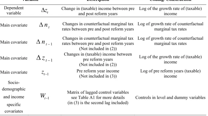
Table 1 gives an overview of the main variables included in the models (2) and (3). Holmlund and Söderström (2011) are the first to emphasize that the common specification in (2) possibly ignores severe econometric problems. The error term in (2) is a first difference, while z_{t1 and} _{t are likely to be correlated. Moreover, the conventional approach does not}

allow for the computation of long- and short-term estimates, estimating only some unknown combination of the two. Even when one controls for the lag structure, results depend on the base year and could be biased. Their approach generalizes conventional empirical specifications by explicitly separating possible short- and long term behavioral responses.15 Following their notation, our first-differenced final dynamic estimation equals:

2

1 1 2 1 1 2

z_t    n_t  (   ) n_t   z_t  W _t   _{t (3).}

Contrary to the Gruber and Saez (2002) model, consistent estimates of (3) are challenged by more than one endogenous variable in 2SLS: 2

t

n

 _, n_t1 and z_t1 . 16 We instrument

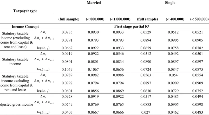
them by constructing counterfactual growth rates for the first steps.17 We use income type specific and aggregate growth rates to derive counterfactual incomes based on the years 2001 and 2002. Relying on sufficient high partial R² values, our instruments for the NTR and lagged income growth are strong in the first stage (See Table A4 in the Appendix for further details). Following Holmlund and Söderström`s notation, we interpret the ₁ coefficient as the short-term elasticity, while the compounded coefficients 1 2

1

  



 determine the long-term

responsiveness.

5 Results

Our estimations are computed by using the income growth between 2003 and 2004 as well as 2003 and 2005. Before we depict regression results, we highlight descriptive statistics for income growth in Table 2. Taxpayers are sorted according to their pre-base year income and are split into different income ranges. Table 2 confirms that standard deviations increase while lagged income decreases (heavily) with increasing income. It indicates high negative

15 _{The complete derivation of the model is given in the Appendix.}

16 _{Possible pitfalls with 2SLS and a discussion of the weak instrument problem can be found in Staiger and Stock}

(1997).

17 _{We follow the common approach in the literature by constructing counterfactual net-of-tax rates from}

counterfactual incomes. Counterfactual incomes are computed by inflated pre reform year income with income-source specific or aggregate growth rates. For the lagged income growth, we derive a counterfactual lagged income growth as instrument.

growth rates among richest taxpayers, even over the whole observation period. In particular, the log of lagged taxable income for married (single) taxpayers with a pre-base year income above 1,000,000 (500,000) EUR reveals unusual growth rates in both lag structures. From 2000 to 2001 the first significant reform step on the marginal tax rates was implemented. Since our data start with assessment year 2001, we are not able to control for the potential bias, resulting from this reform component. However, this might cause a substantial influence on our regression results, especially on the ones of the top income earners.18

[Table 2 about here]

We try to capture estimation results on the largest sample possible. Accounting for the influence of richer taxpayers on our estimates, we apply different cutoff rules at the upper end of the income distribution.19 To account for the top income group’s potential influence we perform additional robustness checks without the top income earners. For married taxpayers we sequentially exclude observations exceeding a taxable income higher than 1,000,000 EUR (800,000 EUR) in 2001 or 2002, cutting nearly 1.1% (4.6%) of the full sample. For single taxpayers we perform robustness checks excluding incomes higher than 500,000 EUR (400,000 EUR) cutting about 2.1% (2.6%) of the single taxpayers observations.20

By including income source specific covariates and socio-demographic covariates, we control for possible sources of heterogeneity among taxpayers. Table A1 in the Appendix describes the socio-demographic and income source specific covariates in greater detail.

Slemrod (1992, 1994 and 1995) derives a hierarchy for behavioral reactions, indicating that ‘real’ behavior is least responsive and closest to long-term estimates.21 For the sake of lucidity, we depict shortened regression output, including the short-term, the long-term elasticity and the coefficients necessary to compute the long-term elasticity.22 We interpret immediate (short-term) responses rather as short-term tax planning than ‘real’ behavioral reactions; while long-term responses are interpret as ‘real’ behavioral changes. Our understanding is the short-term response aims to save income taxes, whereas ‘real’ behavioral changes indicate real individual income growth induced by tax reforms.

18 _{Our panel allows us to identify “the richest taxpayers” on basis of few years only. Since the pre-base years are}

the only years without potential endogeneity, we use them for our cut-off rules.

19 _{Lower and upper cutoff rules are based on the definition of the respective income concept.}

20 _{Since we estimate the income growth 2003 to 2004 and 2003 to 2005, our pre-base years are 2002 and 2001}

respectively.

21 _{According to Slemrod´s considerations, short-term reactions are likely to be driven by a change in reporting}

behavior and/or the timing of transactions. The distinction between long-term and short-term elasticities is of particular interest to compute the impact of habit persistence (see Johnson and Pencavel, 1984). Additionally, taxpayers might not be perfectly informed and need some time to adjust.

Regressions are performed in three dimensions. First, we compute different results for samples, applying the aforementioned cutoff rules. Second we investigate elasticities for four different (tax code related) income aggregates. Third, we split regressions for married and single taxpayers. Main results are presented in section 5.1 (Table 3) and rely on the two most common income concepts. These results are compared with other recent German findings from Gottfried and Witczak (2009). Finally, a sensitivity analysis with two alternative income concepts is given in section 5.2 (Table 4).

5.1 Results for Taxable Income Concepts

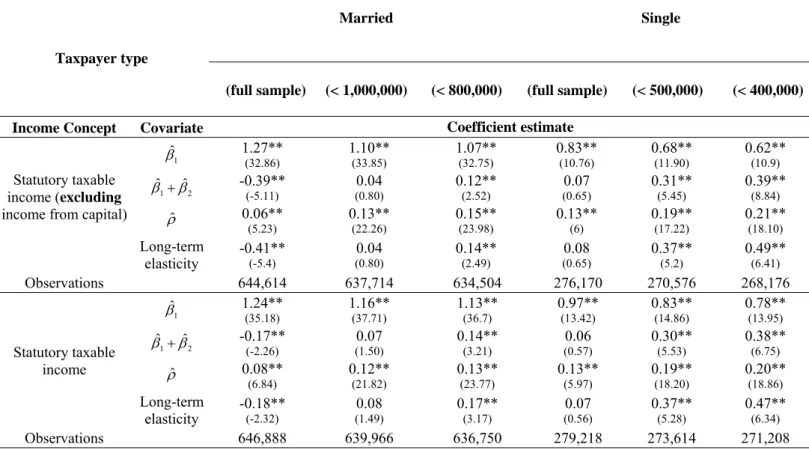
Table 3 depicts regression results in four blocks. The upper two blocks present estimates based on the taxable income excluding income from capital. Results for married taxpayers are shown on the left and for single taxpayers on the right side. The lower two blocks are sorted the same way, but based on the statutory taxable income.

Presented results summarize coefficients of interest, namely the short-term elasticity ˆ1 and

necessary coefficients to derive the long-term elasticity ( ˆ1ˆ2) and ˆ.

Short-term elasticities for married taxpayers are fairly high, significant and robust to cutoff rules exceeding unity with mean 1.14. There is only little variation between the different sample sizes. Moreover, there are no considerable differences for the short-term estimates, when income also includes capital. Long-term elasticities for married taxpayers are (much) smaller and significantly sensitive to income cutoffs at the top. The long-term elasticity is negative for both full samples: -0.41 and -0.18. The lower the top income cutoff is, the stronger the long-term responsiveness. This is observable for both groups of taxpayers. When the cutoff applies for incomes exceeding 800,000 EUR, the long-term elasticity becomes significantly positive, ranging between 0.14 and 0.16. Again, differences between the income concepts are very small.

For single taxpayers short-term reactions are dependent of the sample selection and vary between 0.62 and 0.97. The short-term responsiveness decreases, the lower the cutoff income is. Results are insensitive to the underlying income concepts. For the whole sample long-term elasticties are insignificant, but become statistically significant and increase to approximately 0.50 with cutoff. Overall, the difference between short-term and long-elasticities is more pronounced for married taxpayers than for single taxpayers, while single taxpayer show stronger long-term reactions.

Feldstein (1999) derived a formula to calculate the excess burden of income taxation by ETI. In his setting, the deadweight loss is directly proportional to the ETI with respect to the net-of -tax share.23 Assuming a long-term elasticity of 0.5, the deadweight loss is approximately cut in half, implying only a modest or at least a substantially lower deadweight loss by income taxation than found in previous studies.

We are able to derive several important implications from our findings:

(1) Single and married taxpayers react differently to the income tax reform, supporting separate estimations. This is true for short-term as well as long-term elasticities. The obvious fact is that most jointly assessed taxpayers generate more (taxable) income, resulting in higher economic resources and more allocation flexibility with regard to working time in the long-run. They also benefit from the opportunity of intrapersonal transfers affecting short-term behaviour.

(2) Our results emphasize the useful separation of short-and long-term elasticities. Moreover it supports the hypothesis that short-term responsiveness is heavily influenced by tax planning motives and cannot be regarded as real behavioral changes. This seems to be especially pronounced for married taxpayers.

(3) Long-term behavioral responses are substantially smaller than short-term responses. Estimates for married taxpayers are much smaller than for single taxpayers. In case of the full sample for married taxpayers, we even find negative long-term elasticities. This seems to be mainly driven by high income earners as restricted samples provide another picture, indicating modest positive behavioral responses. Since high income earners should have high tax planning possibilities, these taxpayers seem to pull results below zero.24

(4) Short-term estimates are robust to sample selection, whereas long-term elasticities are very sensitive to the inclusion of richer taxpayers. Gottfried and Witczak (2009) were first to present empirical estimates of the ETI for Germany, applying the approach by Gruber and Saez (2002). Their preferred specification pools single and married taxpayers, controlling with a dummy variable for joint filing. They report an average ETI of 0.6, which is in range of our short-term estimates for single taxpayers but rather in between the short-and long-term elasticities for married. Gottfried and Witczak`s (2009) perform only estimations based on the statutory taxable income, but do not deliver results for the commonly used statutory taxable income without income from capital. They also include some interaction term with the elasticity coefficient in their favored specification. We are not sure how to interpret results based on the described specification. Thus, we believe that our estimation strategy is helpful

23 _{See Feldstein (1999), p. 677.}

to improve the evaluation of the German income tax reform by disentangling one-time from more persistent increases in taxable income. The application of the dynamic approach allows us to control for potential announcement effects. Since the whole reform was well known to taxpayers in advance, our estimation method is eligible to identify more dimensions (immediate and gradual) of behavioral responses for different types of taxpayers.25

5.2 Results for Alternative Income Concepts

For robustness of our estimates and a wider understanding of ETI as a measure for welfare analysis, we vary the underlying income concept in two more ways. First, we compute an alternative taxable income excluding both income from capital and from rent and lease. One can argue that income from rent and lease is also a rather capital intense component and thus very similar to income from capital itself. Moreover, income from capital intense sources possesses more tax planning potential than labor intense sources. Therefore, these incomes are likely to react differently to cuts in marginal tax rates.

Furthermore, we follow Chetty`s (2009) theoretical considerations by estimating behavioural responses to the tax reform with other than purely tax code related income concepts. The construction of a ‘real’ economic income from income tax return data is challenging but still promising.26 Similarly to the approach from Bach et al. (2009),we derive an aggregate gross income, the AGI, from information contained in the income tax returns. 27 _{It differs in a}

whole range of aspects from the taxable income. The construction comprises the sum of all gross incomes, tax reliefs, allowances, specific depreciations, as well as several tax free earnings. This income concept is designed to be a better proxy for the actual consumption possibilities than the (tax code based) income aggregates provided in the data. It allows a more reasonable interpretation of ‘real’ behavioural responses to tax reforms. Table 4 depicts estimates for these alternative income concepts. First we depict results from the taxable income excluding income from capital and rent & lease. Comparing the results from this income definition with estimates from the standard concepts allows investigating the influence of exclusion of the two most capital intense income sources on coefficient estimates. For further robustness check we exclude the same taxpayers, when applying the same cut off rules as described above.

25 _{Due to the flooding of River Oder in 2002, one of the reform steps in 2003 was postponed for one year and}

added to the (planned) reform step in 2004, potentially upwardly biasing elasticities estimates.

26 _{See for example Gruber and Saez (2002) and Giertz (2004, 2010).}

27 _{Since Bach et al. (2009) control for various negative incomes and classify them as pure tax savings; we do not}

incorporate all of their adjustments. Further information on the adjusted gross income construction is given in Table A7 in the Appendix.

Results for the taxable income excluding income from capital and rent & lease differ partially from our preferred specification, i.e. statutory taxable income, depending on the sample size and coefficient estimate. Results for the full samples for married and singles are quite similar in magnitude to the results from the taxable income excluding income from capital. Even results for the short-term elasticities are hardly distinguishable over all samples. However, long-term elasticities are significantly smaller for all of the restricted samples. For married taxpayers long-term elasticities do neither show significant estimates for the two restricted samples. The long-term elasticities for single taxpayers are significantly different from zero. They vary around 0.3 but are also significantly smaller than results from taxable income excluding capital. This is especially interesting because it suggests that income growth, in the long-term, seems to depend highly on the income from rent & lease. Given that this type of income is a common tax planning tool to reduce tax burden, long-term results appear to be driven by this factor. Incomes from rent & lease on average is negative, thus it looks like that negative incomes decline according to the tax reform.

While the estimates for different taxable income concepts show high sensitivity to the inclusion of the richest taxpayers, it is remarkable that coefficients for the AGI are less affected by sample selection. Short-term elasticities are always above unity with pretty similar patterns for married and single taxpayers. Estimates range from 1.27 to 1.23 and 1.21 to 1.34 respectively. Contrary to more tax-code related income measures, there is no clear distinction between immediate responses between these two groups of taxpayers.

With regard to the long-term elasticities, it is remarkable that all estimates are positive and significantly different from zero while still having a substantial difference to the short-term estimates. Comparing results to our preferred specification (in the full sample, Table 3), immediate responses of the married taxpayers are economically not distinguishable: 1.27 versus 1.26, whereas the short-term reactions are severely different: -0.41 versus 0.13. For single taxpayers the long-term elasticity exceeds our preferred long-term elasticity: 0.47 versus 1.01.

It is surprising that the estimates for the AGI concept imply rather higher ‘real’ responses than for the statutory taxable income concept. The AGI tries to comprise income components that are economically more relevant than the taxable income only. While a broad range of applied economic research relies on AGI as an important variable, we are only able to construct our AGI on tax code related data. Since tax code data provide rather a small range of non-tax code related information, our AGI might lack central income components. Moreover, income tax return data just provide vague and implicit details on important aspects such as taxpayers´ wealth, tax-sheltering activities and the consumption of tax-favored goods. We believe that

these missing pieces are decisive and especially affect the growth rate of our AGI, explaining the discrepancies between our empirical findings and expected results from theory. From our sensitivity analysis with the AGI concept we are able to derive two findings: (1) Elasticity estimates are (slightly) bigger than estimates which are based on tax-code related income. We raise doubt if these results reflect real behavioral changes. However, given that AGI comprises more information, these results are nevertheless important for a careful distinction between more economic dimensions and just tax code related. (2) We find that the magnitude of our estimates is more robust, when we control for the influence of taxpayers at the upper end of the income distribution. Results are less sensitive to sample selection, indicating that tax planning potential is not equally distributed among taxpayers but affected by the size of their overall taxable income and its composition.

6 Conclusion

There is still no consensus in literature on the size and influence of marginal tax rate changes on reported taxable income. While ETI holds promises to capture more dimensions of behavioral responses to (income) taxation, its importance for welfare analysis is doubtful. Nevertheless it retains “… the promise of more accurately summarizing the marginal efficiency cost of taxation than a narrower measure of taxpayer response such as the labor supply elasticity.” (See Saez et. al, 2012). Moreover, Slemrod (1998) emphasizes "[ETI] ... is more important than all others, because it summarizes all of what needs to be known for many of the central normative questions of taxation." ETI is still the central parameter for assessment of tax reforms. Disentangling long-term from short-term elasticities also promises to deliver results that are more related to real behavioral responses, serving as an adequate potential proxy for calculation of deadweight losses of progressive taxation.

Our approach is a promising tool to evaluate income tax reforms more profoundly. We contribute to the existing empirical literature on ETI by providing short- and long-term elasticity estimates for Germany. Moreover we derive results from four different income concepts, confirming the common view that only some income sources features considerable taxable income planning potential.

Our findings support the view that there are at least two behavioural effects resulting from an income tax reform: (1) Short-term changes in reporting behaviour. (2) Long-term responsiveness as economic adjustments by taxpayers.

Although the current empirical literature favours the distinction and highlights its importance, the vast majority of previous approaches do not distinguish between long- and short-term reactions. For the German case we pioneer in providing benchmark short-term and long-term

estimates. Results exhibits high sensitivity to the underlying income concepts, cut off rules at the upper end of the income distribution and between married and singles.28 The short-term elasticity of married taxpayers of taxable income to the net-of-tax rate is fairly high, while short-term estimates for single are significantly lower.

Following Giertz (2010), we can confirm that empirical results depend considerably on the concrete empirical model and possible innocuous control variables.29 Chetty (2009) highlights alternative explanations for the wide range of estimates found in the literature. Both the income concepts as well as taxpayers ability to plan and shift income complicates interpretation of ETI. Moreover, Chetty provides a detailed critical discussion, and argues that ETI as the only central measure of welfare analysis is at least not unproblematic. He concludes that high elasticities might result from tax planning and tax avoidance. As robustness check, Chetty proposes the use of other income concepts (in combination with taxable income) to calculate real marginal excess burden of taxation.30 We perform estimations on an alternative income concept and obtain strong(er) results compared to ETI. This finding does not come by surprise since we are using income tax return data, which is only conclusive for some of the income sources. While data quality on income sources like income from employment is very comprehensive, detailed data on other taxable income components is not always available.31 _{Thus, we interpret our AGI results with caution but still}

agree with Chetty.

His vote for theoretical and empirical rigor, i.e. the proper empirical application of theory based multiple alternative income concepts to determine a range of ETI estimates, provides a solid basis for the estimation of short-term and long-term ETI. Future research should also concentrate on the inclusion of sophisticated income control in a dynamic estimation framework to account for divergence within the income distribution and the impact of richer taxpayers. We also believe that there is a substantial need to distinguish between different responses to tax reforms, e.g. increasing real income, changes in reporting behavior, income shifting between spouses, the willingness to itemize and to donate. With more years of

28 _{Long-term elasticities are very sensitive to the exclusion of taxpayers with higher taxable incomes. Short-term}

estimates are similar to the elasticity results from Gottfried and Witczak (2009). Their result is only little smaller than our short-term estimates for married taxpayers. With regard to long-term responses, our findings indicate that persistent behavioral changes are rather modest and imply that marginal tax rate reductions do not significantly increase taxpayers´ (taxable) income. Tax induced permanent income changes appear to be rather small, implying only modest deadweight losses of progressive taxation, raising doubts about tax revenue neutral tax reforms.

29 _{Giertz votes for the need of empirical rigor. However, the literature demonstrates the lack of consistency in}

estimation modeling.

30 _{For example, Gruber and Saez (2002) use a wider income concept than taxable income for robustness analysis.} 31 _{Data for income sources like self-employment or business are limited to profits subject to taxation. Necessary}

observations available, these will be promising steps to identify exogenous economic trends affecting (the components of) ETI.

Table 1. Dependent variable and variables of interest

Variable Description Coding/ Construction

Dependent

variable



z

Main covariate



n

rates between pre and post reform years Log of growth rate of counterfactual marginal tax rates Main covariate



n

Changes in counterfactual marginal tax rates between pre and post reform years

(Not included in (2))

Log of growth rate of counterfactual marginal tax rates

Main covariate



_z

Log of the growth rate of (taxable) income

Main covariate

z

Log of pre reform years (taxable) income Socio- demographic and income specific covariates 1 t

W

Table 2. Growth rates for taxpayers, sorted by pre base year income Lag structure 2001 – 2003 – 2005 2002 – 2003 - 2004 Log of taxable income Log of lagged taxable income Log of taxable income Log of lagged taxable income Taxpayer type Income class (€) N Mean Std-Dev. Mean Std-Dev. N Mean Std-Dev. Mean Std-Dev. Married ≤200,000 6,531,961 0.018 0.272 0.031 0.278 6,532,295 0.010 0.215 0.010 0.216 200,001 – 400,000 44,980 0.030 0.562 -0.013 0.543 44,095 0.023 0.460 -0.069 0.473 400,001 – 600,000 7,035 0.054 0.689 -0.032 0.666 7,199 0.031 0.550 0.539 0.689 600,001 – 800,000 2,455 0.094 0.725 -0.088 0.752 2,443 0.023 0.637 -0.109 0.583 800,001 – 1,000,000 1,131 0.047 0.764 -0.049 0.757 1,219 0.048 0.625 -0.120 0.668 > 1,000,000 2,484 0.088 0.821 -0.142 0.878 2,795 0.075 0.697 -0.122 0.742 Single Income class (€) N Mean Std-Dev. Mean Std-Dev. N Mean Std-Dev. Mean Std-Dev. ≤ 100,000 3,850,706 0.035 0.285 0.074 0.304 3,853,428 0.021 0.234 0.026 0.233 100,001 – 200,000 33,515 -0.007 0.590 0.026 0.578 31,099 0.020 0.490 -0.064 0.479 200,001 – 300,000 5,507 0.004 0.666 -0.003 0.675 5,152 0.036 0.532 -0.083 0.606 300,001 – 400,000 1,890 0.03779 16 0.695 -0.007 0.686 1,831 0.021 0.582 -0.066 0.570 400,001 – 500,000 903 0.023 0.757 -0.065 0.763 831 0.061 0.532 -0.061 0.565 > 500,000 2,087 0.078 0.846 -0.046 0.882 2,257 0.052 0.675 -0.105 0.729 Note: Growth rates are computed using observation weights delivered by the Federal Statistical Office

Table 3. 2SLS estimates for main income concepts, pooled full and restricted samples

Taxpayer type

Married

Single

(full sample) (< 1,000,000) (< 800,000) (full sample) (< 500,000) (< 400,000)

Income Concept Covariate Coefficient estimate

Statutory taxable income (excluding

income from capital)

1 ˆ  1.27** _(32.86) 1.10** _(33.85) 1.07** _(32.75) 0.83** _(10.76) 0.68** _(11.90) 0.62** _(10.9) 1 2 ˆ ˆ   -0.39** _{(-5.11) (0.80)} 0.04 0.12** _{(2.52) (0.65)} 0.07 0.31** _(5.45) 0.39** _(8.84) ˆ  0.06** (5.23) 0.13** (22.26) 0.15** (23.98) 0.13** (6) 0.19** (17.22) 0.21** (18.10) Long-term elasticity -0.41** (-5.4) (0.80) 0.04 0.14** (2.49) (0.65) 0.08 0.37** (5.2) 0.49** (6.41) Observations 644,614 637,714 634,504 276,170 270,576 268,176 Statutory taxable income 1 ˆ  1.24** _(35.18) 1.16** _(37.71) 1.13** _(36.7) 0.97** _(13.42) 0.83** _(14.86) 0.78** _(13.95) 1 2 ˆ ˆ   -0.17** _{(-2.26) (1.50)} 0.07 0.14** _{(3.21) (0.57)} 0.06 0.30** _(5.53) 0.38** _(6.75) ˆ  0.08** (6.84) 0.12** (21.82) 0.13** (23.77) 0.13** (5.97) 0.19** (18.20) 0.20** (18.86) Long-term elasticity -0.18** (-2.32) 0.08 (1.49) 0.17** (3.17) 0.07 (0.56) 0.37** (5.28) 0.47** (6.34) Observations 646,888 639,966 636,750 279,218 273,614 271,208 Note: T values of coefficient estimates in brackets. ** denote a significant level at 99%. Observation numbers vary between income concepts due to technical requirements of the estimation procedure: sub-aggregates of the statutory taxable income might be negative, implying a marginal tax rate of 0. Results are shortened to two decimal places but rely on the un-shorted result.

Table 4. 2SLS estimates for alternative income concepts, pooled full and restricted samples

Taxpayer type

Married

Single

(full sample) (< 1,000,000) (<800,000) (full sample) (< 500,000) (< 400,000)

Income Concept Covariate Coefficient estimate

Taxable income (excluding income

from capital & rent

and lease) 1 ˆ  1.18** _(32.87) 1.05** _(33.23) 1.10** _(32.59) 0.91** _(12.42) 0.70** _(12.74) 0.68** _(12.37) 1 2 ˆ ˆ   -0.37** _{(-5.44) (-0.17)} -0.01 _(1.03) 0.05 _(-1.18) -0.13 0.22** _(3.96) 0.26** _(4.76) ˆ  0.05** (4.24) 0.13** (20.79) 0.14** (21.95) 0.10** (4.40) 0.20** (16.81) 0.21** (16.93) Long-term elasticity -0.39** (-5.74) (-0.17) -0.01 (1.02) 0.05 (-1.21) -0.13 0.27** (3.82) 0.33** (4.53) Observations 631,370 624,484 621,282 266,456 260,988 258,916 Adjusted Gross Income 1 ˆ  1.27** _(32.83) 1.23** _(40.41) 1.26** _(42.33) 1.34** _(15.5) 1.21** _(19.67) 1.20** _(20.19) 1 2 ˆ ˆ   0.27** _(6.74) 0.29** _(8.42) 0.25** _(7.33) 0.75** _(18.81) 0.67** _(18.17) 0.70** _(19.60) ˆ  0.13** (13.89) 0.12** (21.41) 0.13** (23.90) 0.27** (10.16) 0.22** (17.04) 0.26** (19.59) Long-term elasticity 0.31** (6.97) 0.33** (8.50) 0.28** (7.39) 1.01** (16.57) 0.85** (17.67) 0.95** (18.49) Observations 644,622 637,722 634,512 276,180 270,586 258,670 Note: T values of coefficient estimates in brackets. ** denote a significant level at 99%. Observation numbers vary between income concepts due to technical requirements of the estimation procedure: sub-aggregates of the statutory taxable income might be negative, implying a marginal tax rate of 0. Results are shortened to two decimal places but rely on the un-shorted result.

Appendix

Derivation of the dynamic model.

The basic model:

1 2 1 2 1

z_t     n_t   n_t







First differencing of the basic model leads to:

1 2 1 2 1 2

z_t  











 

The rearrangement of the specification gives us the final model specification:

1 1 2 1 2 1

2

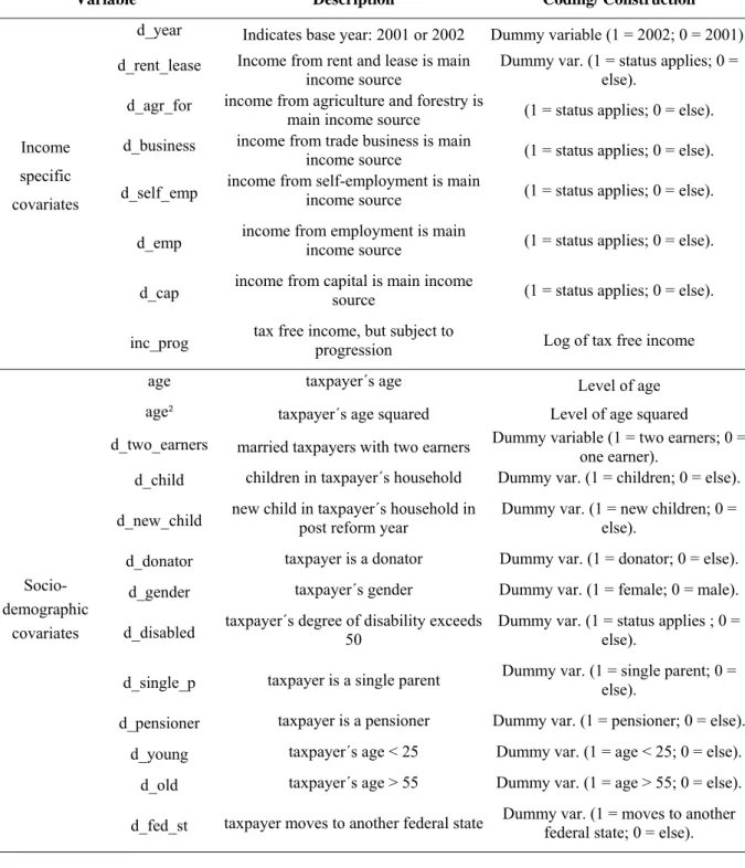
Table A1. Independent covariates

Variable Description Coding/ Construction

Income specific covariates

d_year _{Indicates base year: 2001 or 2002 Dummy variable (1 = 2002; 0 = 2001).} d_rent_lease Income from rent and lease is main

income source Dummy var. (1 = status applies; 0 = else). d_agr_for income from agriculture and forestry is

main income source (1 = status applies; 0 = else). d_business income from trade business is main

income source (1 = status applies; 0 = else). d_self_emp income from self-employment is main _{income source} (1 = status applies; 0 = else). d_emp income from employment is main _{income source} (1 = status applies; 0 = else). d_cap income from capital is main income _source (1 = status applies; 0 = else). inc_prog tax free income, but subject to _progression Log of tax free income

Socio- demographic

covariates

age taxpayer´s age _{Level of age} age² _{taxpayer´s age squared Level of age squared}

d_two_earners _{married taxpayers with two earners} Dummy variable (1 = two earners; 0 = one earner).

d_child children in taxpayer´s household Dummy var. (1 = children; 0 = else). d_new_child new child in taxpayer´s household in _{post reform year} Dummy var. (1 = new children; 0 = _else).

d_donator taxpayer is a donator Dummy var. (1 = donator; 0 = else). d_gender taxpayer´s gender Dummy var. (1 = female; 0 = male). d_disabled taxpayer´s degree of disability exceeds ₅₀ Dummy var. (1 = status applies ; 0 = _else). d_single_p taxpayer is a single parent Dummy var. (1 = single parent; 0 = _else). d_pensioner taxpayer is a pensioner Dummy var. (1 = pensioner; 0 = else).

d_young taxpayer´s age < 25 Dummy var. (1 = age < 25; 0 = else). d_old taxpayer´s age > 55 Dummy var. (1 = age > 55; 0 = else). d_fed_st taxpayer moves to another federal state Dummy var. (1 = moves to another _{federal state; 0 = else).}

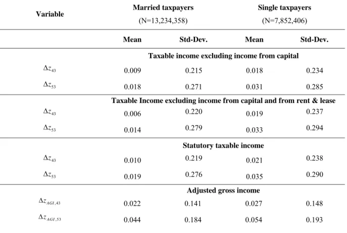
Table A2. Mean growth rates, Weighted Observations

Variable Married taxpayers

(N=13,234,358)

Single taxpayers

(N=7,852,406)

Mean Std-Dev. Mean Std-Dev. Taxable income excluding income from capital

43 z  _{0.009 0.215 0.018 0.234} 53 z  _{0.018 0.271 0.031 0.285}

Taxable Income excluding income from capital and from rent & lease

43 z  _0.006 0.220 _0.019 0.237 53 z  _{0.014 0.279 0.033 0.294}

Statutory taxable income

43 z  _0.010 0.219 _0.021 0.238 53 z  _0.019 0.276 _0.035 0.290

Adjusted gross income

,43 AGI z  _{0.022 0.141 0.027 0.148} ,53 AGI z  _{0.044 0.184 0.054 0.193}

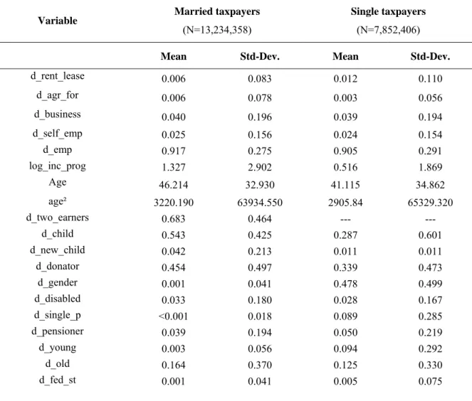
Table A3. Socio-demographic variables, Weighted Observations

Variable Married taxpayers

(N=13,234,358)

Single taxpayers

(N=7,852,406)

Mean Std-Dev. Mean Std-Dev.

d_rent_lease _{0.006 0.083 0.012 0.110} d_agr_for _{0.006 0.078 0.003 0.056} d_business _{0.040 0.196 0.039 0.194} d_self_emp 0.025 0.156 0.024 0.154 d_emp 0.917 0.275 0.905 0.291 log_inc_prog 1.327 2.902 0.516 1.869 Age _{46.214 32.930 41.115 34.862} age² 3220.190 63934.550 2905.84 65329.320 d_two_earners _{0.683 0.464 --- ---} d_child 0.543 0.425 0.287 0.601 d_new_child 0.042 0.213 0.011 0.011 d_donator 0.454 0.497 0.339 0.473 d_gender 0.001 0.041 0.478 0.499 d_disabled 0.033 0.180 0.028 0.167 d_single_p <0.001 0.018 0.089 0.285 d_pensioner _{0.039 0.194 0.050 0.219} d_young _{0.003 0.056 0.094 0.292} d_old _{0.164 0.370 0.125 0.330} d_fed_st 0.001 0.041 0.005 0.075

Table A4. First stage partial R²

Taxpayer type

Married

Single

(full sample) (< 800,000) (<1,000,000) (full sample) (< 400,000) (< 500,000)

Income Concept First stage partial R²

Statutory taxable income (excluding income from capital &

rent and lease)

t n  0.0935 0.0930 0.0933 0.0529 0.0512 0.0521 1 t t n n_    0.0791 0.0793 0.0793 0.0894 0.0905 0.0905 1 lo g(zt ) 0.0662 0.0922 0.0933 0.0659 0.0758 0.0782 Statutory taxable income t n  0.0919 0.0922 0.0546 0.0512 0.0492 0.0501 1 t t n n_    0.0801 0.0801 0.0834 0.0890 0.0897 0.0897 1 lo g(zt ) 0.1059 0.1067 0.0656 0.0724 0.0847 0.0875 Statutory taxable income excluding income from capital &

rent and lease

t n  0.0989 0.0982 0.0986 0.0563 0.054 0.0554 1 t t n n_    0.0792 0.0794 0.0794 0.0897 0.0909 0.0909 1 lo g(zt ) 0.0601 0.0856 0.0869 0.0630 0.0729 0.0752

Adjusted gross income

t n  0.0928 0.0919 0.0922 0.0517 0.0485 0.0494 1 t t n n_    0.0749 0.0769 0.0765 0.0883 0.0905 0.0898 1 lo g(zt ) 0.0405 0.0667 0.0666 0.027 0.0462 0.0483

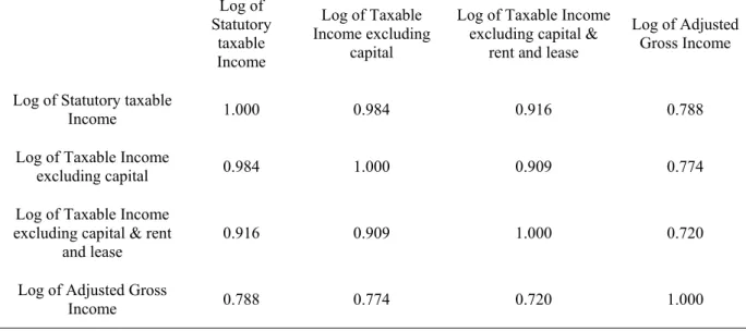
Table A5. Correlation Matrix, Pooled Married Taxpayers (N=13,234,358) Log of Statutory taxable Income Log of Taxable Income excluding capital

Log of Taxable Income excluding capital &

rent and lease

Log of Adjusted Gross Income Log of Statutory taxable

Income 1.000 0.984 0.916 0.788

Log of Taxable Income

excluding capital 0.984 1.000 0.909 0.774 Log of Taxable Income

excluding capital & rent

and lease 0.916 0.909 1.000 0.720

Log of Adjusted Gross

Income 0.788 0.774 0.720 1.000 Single taxpayers (N=7,852,406) Log of Statutory taxable Income Log of Taxable Income excluding capital

Log of Taxable Income excluding capital &

rent and lease

Log of Adjusted Gross Income Log of Statutory taxable

Income 1.000 0.976 0.915 0.772

Log of Taxable Income

excluding capital 0.976 1.000 0.904 0.757 Log of Taxable Income

excluding capital & rent

and lease 0.915 0.904 1.000 0.707

Log of Adjusted Gross

Table A6. Adjusted gross income

Income from business activity

(including income from agriculture and forestry, from unincorporated business enterprise and from self-employed activities) + wage income, income from renting and leasing and other income

+ earnings from capital investments (imputation of missing data on an average level) + all tax reliefs and tax allowances for income from business activity as far as identifiable

+ allowable expenses for wage and other income (consumptive character) + age relief

+ tax-exempted income from foreign countries + loan and income indemnification

+ life annuity income less income component (flat 70% of life annuity income) + tax shelters: losses from equity holdings

+ losses from business activity income and renting and leasing income, if the modified income class and the sum of income until this point is still negative (negative consumption is not possible)

- fixed income tax and solidarity surcharge - alimony / child support

+ child benefit

Table A7. 2SLS estimates for statutory taxable income excluding income from capital

Taxpayer type

Married Single

(full sample) (<1,000,000) (<800,000) (full sample) (<500,000) (<400,000)

Income Concept Covariate Coefficient estimate

Statutory taxable income (excluding

income from capital)

Constant _(26.148) 0.187** _(26.901) 0.191** _(27.406) 0.195** _(22.417) 0.193** _(22.581) 0.191** _(22.887) 0.193** 1 ˆ  _(32.863) 1.271** _(33.845) 1.104** _(32.753) 1.066** _(10.762) 0.827** _(11.900) 0.681** _(10.897) 0.622** 1 2 ˆ ˆ   -0.387** _{(-5.114) (0.803)} 0.038 0.119** _{(2.516) (0.654)} 0.072 0.306** _(5.451) 0.390** _(8.844) ˆ  0.055** (5.225) (22.263) 0.133** (23.982) 0.146** 0.125** (5.995) (17.223) 0.187** (18.102) 0.207** Long-term elasticity -0.405** (-5.395) (0.800) 0.043 0.139** (2.488) (0.645) 0.082 0.371** (5.197) 0.485** (6.405) d_year -0.022** (-11.923) -0.017** (-9.960) -0.015** (9.258) -0.004 (-1.419) -0.001 (-0.364) <0.001 (0.351) d_rent_lease -0.001 (0.228) (-0.277) -0.001 (-0.637) -0.004 -0.038** (-5.115) -0.034** (-4.109) -0.030** (-4.020) d_agr_for -0.070** (9.802) 0.067** (9.548) 0.065** (9.184) 0.058** (5.227) 0.065** (5.923) 0.063** (5.751) d_business -0.026** (-4.652) -0.025** (-4.293) -0.026** (-4.573) -0.042** (-6.159) -0.034** (-5.043) -0.035** (-5.222) d_self_emp -0.059** (-10.349) -0.053** (-9.308) -0.054** (-9.399) -0.048** (6.867) -0.039** (-5.640) -0.039** (-5.617) d_emp -0.059** (-10.349) -0.055** (9.902) -0.057** (-10.285) -0.085** (13.240) -0.080** (-12.455) -0.081** (-12.611) inc_prog 0.006** (26.622) (25.788) 0.006** (25.487) 0.005** (11.605) 0.006** (11.355) 0.005** (10.899) 0.005** age -0.003** (-38.928) (-39.633) -0.003** (-39.889) -0.003** (-23.489) -0.002** (-23.459) -0.002** (-23.246) -0.002** age² <0.001** (39.004) <0.001** (39.707) <0.001** (39.962) <0.001** (23.460) <0.001** (23.451) <0.001** (23.250) d_two_earners -0.034** (-31.429) (-30.652) -0.032** (-30.516) -0.032** --- --- --- d_child 0.015** (22.758) (23.567) 0.015** (23.729) 0.015** 0.009** (6.683) 0.009** (6.753) 0.009** (6.558) d_new_child -0.008** (-2.669) -0.009** (-3.300) -0.009** (-3.171) -0.020** (-3.276) -0.020** (-3.358) -0.019** (-3.137) d_donator 0.006** (5.760) 0.008** (7.376) 0.008** (7.761) 0.003** (2.047) 0.004** (2.364) 0.003** (2.166) d_gender -0.047** (-4.081) -0.055** (-4.756) -0.054** (-4.659) -0.013** (-7.236) -0.013** (-7.810) -0.014** (-8.127) d_disabled 0.013** (4.206) 0.010** (3.500) 0.010** (3.497) (-0.347) -0.001 (-0.605) -0.003 (-0.060) -0.003 d_single_p -0.017 (-0.716) (-0.686) -0.016 (-0.675) -0.016 (10.010) 0.033** 0.031** (9.636) 0.032** (9.754) d_pensioner -0.036** (-10.067) -0.033** (-9.275) -0.033** (-9.370) 0.033** (6.647) 0.037** (7.464) 0.036** (7.169) d_young -0.056** (-4.478) -0.057** (-4.648) -0.059** (-4.822) -0.010** (-2.625) -0.012** (-3.401) -0.013** (-3.566) d_old -0.014** (-7.547) -0.012** (-6.903) -0.012** (-6.724) -0.012** (-3.195) -0.012** (-3.337) -0.013** (-3.481) d_fed_st 0.027 (1.677) 0.023 (1.416) 0.022 (1.415) 0.038** (3.519) 0.035** (3.344) 0.034** (3.269) Observations 644,614 634,504 637,714 276,170 270,576 268,176 Note: T values of coefficient estimates in brackets. ** denote a significant level at 99%.

Table A8. 2SLS estimates for statutory taxable income

Taxpayer type

Married Single

(full sample) (<1,000,000) (<800,000) (full sample) (<500,000) (<400,000)

Income Concept Covariate Coefficient estimate

Statutory taxable income Constant _(27.232) 0.178** _(27.739) 0.181** _(28.085) 0.183** _(21.877) 0.190** _(21.567) 0.185** _(21.395) 0.184** 1 ˆ  _(35.177) 1.243** _(37.713) 1.158** _(36.698) 1.125** _(12.419) 0.913** _(11.988) 0.661** _(12.714) 0.704** 1 2 ˆ ˆ   -0.168** _{(-2.264) (1.500)} 0.067 0.144** _{(3.207) (-1.176)} -0.128 0.285** _(5.130) 0.221** _(4.031) ˆ  0.076** (6.835) (21.817) 0.121** (23.771) 0.134** 0.100** (4.400) (17.412) 0.212** (16.916) 0.196** Long-term elasticity -0.181** (-2.319) (1.491) 0.075 0.166** (3.165) (-1.209) -0.134 0.361** (4.868) 0.274** (3.883) d_year -0.017** (-9.604) -0.014** (-8.823) -0.013** (-8.132) -0.010** (-3.264) -0.003 (-1.308) -0.005 (-1.871) d_rent_lease 0.007 (1.248) (1.319) 0.007 (1.109) 0.006 -0.042** (-3.333) (1.673) -0.020 (-1.801) -0.022 d_agr_for 0.077** (11.731) (11.707) 0.076** (11.478) 0.074** 0.058** (5.247) 0.064** (5.894) 0.067** (6.093)

d_business -0.012** (-2.361) -0.012** (-2.346) -0.013** (-2.541) -0.036** (-5.144) -0.028** (-4.002) -0.026** (-3.838) d_self_emp -0.044** (-8.678) -0.039** (-8.149) -0.042** (-8.141) -0.048** (-6.610) -0.037** (-5.226) -0.037** (-5.168) d_emp -0.040** (-8.080) -0.039** (-7.976) -0.041** (-8.244) (-11.741) -0.079** (-11.096) -0.074** (-10.859) -0.072** inc_prog 0.006** (26.189) 0.005** (26.249) 0.005** (25.994) 0.006** (13.285) 0.005** (12.485) 0.006** (12.832) age -0.003** (-42.378) (-43.080) -0.003** (-43.256) -0.003** (-25.578) -0.003** -0.002** (24.535) (-24.965) -0.002** age² <0.001** (43.354) <0.001** (43.053) <0.001** (43.229) <0.001** (25.472) <0.001** (24.461) <0.001** (24.881) d_two_earners -0.033** (-32.147) (-31.523) -0.032** (-31.341) -0.032** --- --- --- d_child 0.015** (23.945) (24.563) 0.015** (24.775) 0.015** 0.011** (7.954) 0.010** (7.379) 0.010** (7.694) d_new_child -0.010** (-3.567) -0.011** (-3.933) -0.011** (-31.341) -0.020** (-3.429) -0.019** (-3.255) -0.020** (-3.424) d_donator 0.006** (6.120) 0.007** (6.948) 0.079** (7.336) (0.612) 0.001 (1.093) 0.001 (1.256) 0.002 d_gender -0.045** (-4.064) -0.050** (-4.459) -0.048** (-4.354) -0.009** (-5.575) -0.011** (-6.809) -0.011** (-6.456) d_disabled 0.001** (3.738) 0.009** (3.227) 0.009** (3.232) 0.001 (0.218) -0.001 (-0.229) -0.001 (-0.226) d_single_p -0.013 (-0.556) (-0.599) -0.014 (-0.591) -0.013 (10.867) 0.035** (10.580) 0.034** (10.411) 0.033** d_pensioner -0.027** (-8.087) -0.026** (-7.682) -0.026** (-7.721) 0.023** (4.261) 0.027** (4.942) 0.027** (4.972’) d_young -0.061** (-5.062) -0.062** (-5.145) -0.063** (-5.313) -0.010** (-2.841) -0.013** (-3.839) -0.013** (-3.869) d_old -0.012** (-7.098) -0.062** (-5.145) -0.011** (-6.403) (-1.412) -0.005 -0.007** (-2.039) -0.007** (-1.988) d_fed_st 0.021 (1.325) 0.018 (1.212) 0.017 (1.163) 0.040** (3.785) 0.035** (3.416) 0.035** (3.466) Observations 646,888 639,966 636,750 266,456 258,916 261,174 Note: T values of coefficient estimates in brackets. ** denote a significant level at 99%.

Table A9. 2SLS estimates for statutory taxable income excluding income from capital and

rent and lease

Taxpayer type

Married Single

(full sample) (<1,000,000) (<800,000) (full sample) (<500,000) (<400,000)

Income Concept Covariate Coefficient estimate

Statutory taxable income (excluding

income from capital

& rent and lease)

Constant _(26.386) 0.192** _(26.693) 0.194** 0.199** (27.389) (21.877) 0.190** 0.184** (21.386) (21.485) 0.185** 1 ˆ  _(32.872) 1.177** _(33.226) 1.046** 1.021** (32.590) 0.913** (12.419) 0.705** (12.738) (12.369) 0.682** 1 2 ˆ ˆ   -0.374** _{(-5.442) (-0.173)} -0.008 0.046 (1.025) (-1.176) -0.128 0.218** (3.958) 0.263** (4.757) ˆ  0.046** (4.235) 0.130** (20.791) 0.140** _(21.945) 0.100** _(4.400) 0.196** (16.808) 0.206** (16.935) Long-term elasticity -0.392** (-5.735) -0.250** (-4.302) (1.021) 0.053 (-1.209) -0.134 0.271** (3.815) 0.331** (4.534) d_year -0.023** (-12.683) (-11.235) -0.019** -0.018** (-10.828) -0.010** (-3.264) -0.005 (-1.888) (-1.538) -0.004 d_rent_lease <-0.001 (-0.098) 0.009 (1.002) 0.007 _(0.810) -0.042** _(-3.333) -0.022 (-1.764) -0.022 (-1.751) d_agr_for 0.077** (10.473) 0.074** (10.151) 0.070** _(9.651) 0.058** _(5.247) 0.068** (6.151) 0.066** (5.98) d_business -0.020** (-3.434) -0.022** (-3.652) -0.026** _(-4.342) -0.036** _(-5.144) -0.026** (-3.703) -0.027** (-3.853) d_self_emp -0.055** (-9.246) -0.053** (-8.962) -0.057** _(-9.511) -0.048** _(-6.610) -0.036** (-5.026) -0.037** (-5.168) d_emp -0.046** (-7.941) -0.048** (-8.281) -0.053** _{(-9.046) (-11.741)} -0.079** -0.072** (-10.79) -0.074** (-11.023) inc_prog 0.006** (26.320) (26.010) 0.005** 0.006** _(25.85) (13.285) 0.006** 0.006** (12.866) (12.605) 0.006** age -0.003** (-43.637) -0.004** (-43.746) -0.004** _{(-43.936) (-25.578)} -0.003** (-25.083) -0.003** (-24.673) -0.003** age² <0.001** (46.691) <0.001** (43.808) <0.001** _(43.999) <0.001** _(25.472) <0.001** (24.998) <0.001** (24.595) d_two_earners -0.030** (-29.005) -0.029** (-28.109) -0.029** _(-27.951) --- --- d_child 0.015** (23.874) 0.016** (24.4481) 0.016** _(24.71) 0.001** _(7.954) 0.011** (7.646) 0.010** (7.396) d_new_child -0.009** (-3.195) -0.011** (-3.762) -0.011** _(-3.69) -0.020** _(-3.429) -0.020** (-3.433) -0.019** (-3.25) d_donator 0.004** (3.780) 0.005** (5.197) 0.006** _(5.478) (0.612) 0.001 0.002 (1.226) 0.0019 (1.084) d_gender -0.066** (-5.412) 0.006** (5.245) -0.07** _(-5.710) -0.009** _(-5.575) -0.011** (-6.422) -0.011** (-6.689) d_disabled 0.013** (4.428) -0.071** (-5.798) 0.012** _{(3.951) (0.218)} 0.001 (-0.078) <-0.001 (0.111) 0.001 d_single_p -0.015 (-0.649) 0.012** (3.860) -0.017 _{(-0.738) (10.867)} 0.035** (10.463) 0.034** (10.613) 0.034** d_pensioner -0.038** (-10.347) -0.017 (-0.7231) -0.033** _(-8.97) 0.023** _(4.261) 0.027** (5.0185) 0.028** (5.181)

d_young -0.060** (-4.949) -0.033** (-8.966) -0.062** _(-5.16) -0.010** _(-2.841) -0.014** (-3.894) -0.013** (-3.745) d_old -0.015** (-8.200) -0.06** (-5.001) -0.014** _{(-7.56) (-1.412)} -0.005 (-1.908) -0.007 -0.008** (-2.012) d_fed_st 0.029 (1.869) 0.028 (1.775) 0.027 _(1.746) 0.004** _(3.785) 0.036** (3.466) 0.036** (3.453) Observations 644,622 637,722 634,512 276,180 270,586 258,670 Note: T values of coefficient estimates in brackets. ** denote a significant level at 99%.

Table A10. 2SLS estimates for adjusted gross income

Taxpayer type

Married Single

(full sample) (<1,000,000) (<800,000) (full sample) (<500,000) (<400,000)

Income Concept Covariate Coefficient estimate

Adjusted gross income Constant _(25.334) 0.160** _(27.299) 0.161** _(27.091) 0.159** _(11.488) 0.116** _(16.034) 0.121** _(15.154) 0.113** 1 ˆ  _(32.827) 1.269** _(40.413) 1.227** _(42.331) 1.261** _(15.495) 1.343** _(19.665) 1.205** _(20.193) 1.202** 1 2 ˆ ˆ   0.274** _(6.741) 0.287** _(8.420) 0.245** _{(7.329) (18.808)} 0.745** _(18.172) 0.669** _(19.601) 0.702** ˆ  0.125** (13.889) (21.410) 0.120** (23.900) 0.134** (10.158) 0.273** (17.038) 0.217** (19.593) 0.261** Long-term elasticity 0.313** (6.970) 0.326** (8.502) 0.282** (7.389) (16.567) 1.010** (17.671) 0.854** (18.486) 0.949** d_year -0.009** (-4.486) -0.010** (-6.237) -0.010** (-6.237) -0.014** (-3.191) -0.008** (-2.645) -0.009** (-3.197) d_rent_lease -0.012** (-2.352) -0.011** (-2.095) -0.011** (-2.095) -0.042** (-6.996) -0.031** (-5.342) -0.030** (-5.073)