Off-farm income: evaluating the effects of off-farm income on debt repayment capacity

(1)

Off-farm income: evaluating the effects of off- farm income on debt repayment capacity

by

AARON A. CLING B.S., Iowa State University, 2013

A THESIS

Submitted in partial fulfillment of the requirements for the degree

MASTER OF AGRIBUSINESS Department of Agricultural Economics

College of Agriculture KANSAS STATE UNIVERSITY

Manhattan, Kansas 2017

Approved by:

Major Professor Dr. Allen Featherstone

(2)

ABSTRACT

This thesis examines the effect of off-farm income on a farming operation’s ability to repay their debt. The thesis develops a regression model that includes net farm income, debt repayment capacity with carryover working capital, off-farm income sources and a number of other independent variables that help define each individual borrower. The model provides an evaluation of the current farming environment and examines various income opportunities available to borrowers affects repayment capacity.

This study found that the presence of off-farm income can increase the probability that the operation will be able to repay their debts. The model indicates that if off-farm income is present, the borrower’s debt repayment capacity ratio increases. This thesis further explores the model and the results produced from not only off-farm income but several different variables within the borrower’s scope of business.

Results suggest that many other factors that are not available in the sample also play a large role in predicting an operation’s ability to repay debt. The study determined that the presence of one source of off-farm income was positive and statistically

significant in explaining repayment capacity. An operation with a strong outside income source and one spouse working full time on the farm is more financially stable and will likely be more successful at repaying their debts.

(3)

iii

LIST OF FIGURES

Figure 5.1 Number of Off-farm jobs in 2016 ... 15

Figure 6.1 Debt Repayment Capacity Ratios ... 21

Figure 6.2 Cumulative Density of Debt Repayment Capacity ... 22

Figure 6.3 Debt Repayment Capacity with Carryover Ratio ... 24

Figure 6.4 Cumulative Density of Debt Repayment Capacity with Carryover ... 26

(5)

v

LIST OF TABLES

Table 4.1 Variables Included in the Regression Model of Repayment Capacity ... 11 Table 5.1 Summary Statistics of Southeast Iowa Farm Borrowers ... 16 Table 5.2 Regression Variable Description and Expected Signs for Capacity Model . 17 Table 5.3 Regression Variable Description and Expected Signs for Carryover

Model ... 18 Table 6.1 Regression Output for Capacity Model, Debt Repayment Capacity ... 20 Table 6.2 Regression Output for Carryover Model, Debt Repayment with

(6)

vi

ACKNOWLEDGMENTS

I would like to thank Dr. Allen Featherstone for guidance and reinforcement throughout this entire MAB program and the thesis writing process. Additionally, I appreciate the time and input from Dr. Elizabeth Yeager and Dr. Brian Briggeman. I would also like to thank Deborah Kohl, Mary Emerson-Bowen, and Gloria Burget for all of their encouragement and advice throughout this project and the entire MAB program. Each of them have had a positive impact on my MAB experience and continue to be champions of the program. Kansas State University is lucky to have each of these individuals as part of their organization.

Additionally, I appreciate the support of my employer. They have supported me through the MAB program, and this thesis would not have been possible without their cooperation. This thesis will provide support for our current agricultural portfolio, and guidance when evaluating potential borrowers.

Furthermore, I appreciate the support from the classmates, friends, and family throughout the thesis writing, and every step of the MAB program. I would like to

specifically thank two close friends and classmates, Skylar Rinker and Andrew Lauver. We started this journey together and I have been able to count on them every step of the way, which I am very grateful for. Finally, I owe many thanks to my wife, Abby. Her love, support, and continual encouragement has been vital in my completion of this program.

(7)

1

CHAPTER I: INTRODUCTION

Agricultural income at the farm gate has significantly decreased along with commodity prices over the last four years. Input prices have stayed high and family living expenses remained high as well. Corn and soybean prices reached record levels during 2012, a drought year (Adonizio, Kook and Royales 2012). This led to high input prices, high machinery costs, high cash rent and high land prices. Expenses have not fallen as fast as commodity prices have following a few high production years. This has resulted in low incomes for producers in the United States and many farmers are needing to return to profitability.

Previously, it was rare for a farmer to have an off-farm job. The tasks around the farm were so labor intensive that the entire family would work to complete the necessary tasks. With the modern mechanization of farming and farm equipment, an individual can accomplish much more in a day than an entire family could fifty years ago. However, mechanization comes at a cost. Farmers must generate more cash flow to cover machinery costs. Some new combines and tractors are more than $400,000, land prices are near $10,000 per acre and other nonland costs are also high.

There are two ways to generate more revenue: get bigger or generate income from alternative sources. One way to generate more cash flow is to increase the number of acres in the operation. To make room for a son, daughter, son-in-law, or other family member, the farm often expands. However, obtaining land to expand is not always easy. There’s a finite amount of land available, and if one farm is getting larger that means that another farm is getting smaller or exiting. Taking an off farm job has also been a way for farm families to increase income. This option was important during the farm crisis of the 1980s.

(8)

2

Farm spouses took jobs outside of the house and many farmers did too. Today off-farm income is more common. Often the wife or both the husband and wife work off-farm to bring in an income and to give the family access to healthcare. This generates funds that can be used for debt service and other expenses, but it takes a considerable amount of time away from the farm operation.

In this thesis, financial performance and ratios of farms with off-farm income is compared to farms with no off-farm income. These farms are located in Southeast Iowa and are customers of ABC Bank and Trust. The purpose is to provide loan officers at ABC Bank and Trust and farm client’s information that will aid them in making long-term decisions about their farm operations. The clients have three options: both husband and wife work on the farm; one spouse works full time off the farm; or, both husband and wife work full time off the farm while maintaining the farming operation.

The objective of this thesis to evaluate the importance an off-farm job is to a farming enterprise and help lenders and farmers make long-term decisions about their farming operation. This thesis will evaluate the current ratio, debt repayment capacity, debt repayment capacity with carryover, and several other financial ratios to compare the

(9)

3

CHAPTER II: LITERATURE REVIEW

Debt repayment capacity is a key component when making a loan. The agricultural lending process can be more complex than a traditional consumer loan due to a variety of income sources and expense categories. Before extending a loan to a borrower, the lender must conduct due diligence to ensure the borrower is capable of generating the income required to service that debt. Over the last half century in agriculture, off-farm income has increased in terms of total farm household income (Briggeman 2011). Therefore, it can be assumed that farm households have become increasingly dependent on off-farm income to service their debt.

The three major factors that contribute to debt repayment capacity are income, expenses, and total debt commitment. Of those three segments, this thesis examines the income portion: how it is comprised, and how that affects an operation’s bottom line. The income for a farming operation is derived from: crops, livestock, custom work, and off-farm income. Levels of income from each of these segments varies from operation to operation, but the general theme is the same throughout the United States.

Off-farm income accounts for a larger percentage of income than farm income in many operator households. Every year, USDA reports a large number of operator

households have negative farm income and attribute more than 100% of their annual earnings to off-farm income. Over two million operator households were surveyed and approximately seventy-five percent of them reported that less than one quarter of household income was from farming (USDA 2015). A review of these statistics should encourage lenders to consider the importance of off-farm income when calculating the debt

(10)

4

repayment capacity. The agricultural sector pays close attention to the markets and growing conditions, however off-farm income may play a large role in debt service.

A projected cash flow model can be used as an indicator of client performance and debt repayment capacity over the course of a business cycle. There are many variables that must be considered when developing a cash flow because of unforeseen shocks throughout the life of a loan. These changes could occur in either the expense or income column, but both have an affect on debt repayment capacity. Most farm expenses such as crop inputs are often known at planting with the exception of repairs or unexpected costs that may arise during the year. Farm income can be much more difficult to project. Fluctuating markets, drought, disease, floods, foreign markets, government policy, and many other variables have a large impact on a farm’s income during just one growing season. These variables, among others, make it difficult to develop an accurate cash flow statement to determine if a client is capable of servicing a certain level of debt. If a farm client has off-farm income, it can provide some stability to the annual projections. While an off-farm job can bring its own risk, the income from an annual salary is easier to predict than the income from a corn crop or a herd of cattle. In addition to stability, most farm households depend on off-farm income to service their debt. Nearly all operations with less than $1 million in annual farm receipts require off-farm income to service farm debt (Briggeman 2011).

When evaluating an operation’s annual expenses, it is important to use accurate family living expenses when developing a cash flow. When building a cash flow model for a large operation, living expenses may not have an effect on the bottom line. However, living expenses are not insignificant. A survey of over one thousand farm families that are members of the Illinois Farm Business Farm Management Association showed the average

(11)

5

family living expense in 2015 was $84,779 (Zwilling, Krapf and Raab 2016). While this average may be useful as a starting point, the cost of living varies greatly from operation to operation. The size of family, entertainment, quality of life, and healthcare are all factors to be considered when calculating family living. Of the expenses listed, one that can

significantly affect off-farm employment is health care. If one of the earners of a household has an off-farm job that provides the family with health insurance, it can significantly reduce family living expenses. Other benefits from off-farm employment may need to be considered as well when calculating profit available for debt service. A company vehicle, cell phone, internet access, and many other benefits are common with some off-farm employment that could all positively affect debt repayment capacity.

Those factors and have an impact on an operation’s debt repayment capacity ratio (DRC). Debt repayment capacity is calculated as net income divided by total principal and interest payments due in that time period. The debt repayment capacity ratio does not look at a borrower’s history, but instead it measures their ability to service debt, or potential debt, in current market conditions. Throughout the thesis, debt repayment capacity is calculated with and without off-farm income to show the average operation’s ability to service their debt and how that can be adversely affected with the loss of off-farm employment.

This literature review concentrated on off-farm income, debt repayment capacity, and family living expenses. In general, the size of the farm, age of the producer, and level of diversification affect how dependent the operation is on off-farm income. Additionally, research conducted by other individuals and organizations were beneficial when

(12)

6

CHAPTER III: DEBT REPAYMENT

The main objective of the thesis is to examine the effect of off-farm income on the capital debt repayment capacity of a farming operation. Off-farm employment can

supplement the debt repayment capacity of a farming operation, by increasing liquidity from the added stream of revenue . This chapter will integrate the concepts of off-farm diversification and imperfect knowledge of the future to assess the benefit of off-farm income in a farming operation.

Repayment capacity is determined by an operation’s ability to service debt. Market conditions have a large affect on an operation’s sustainability. While annual cash flow should be predicted as accurately as possible, it can change by the end of a business day with an unexpected move in the commodity markets. Weather, unexpected expenses, and the fluctuation of input costs can all have an impact on a cash flow model and ultimately that borrower’s ability to service their debt.

A borrower’s debt repayment capacity is measured as a ratio and can be calculated as the borrower’s net income divided by total principal and interest payments due in the time period the cash flow encompasses. Debt is defined as the sum of all principal and interest payments that are required in the time period of the cash flow. The balance available is then divided by the total debt payments due to calculate the debt repayment capacity ratio. For example, an operation with a net income of $150,000 and a total debt load of $100,000 would have a repayment ratio of 1.5. This ratio suggests that if the cash flow is accurate, the borrower will be able to make all their required payments for the year, and will have an additional 50% in net working capital.

(13)

7

A borrower’s debt repayment capacity with carryover working capital (DRCC) is a ratio and that is calculated as the borrower’s net income plus current working capital divided by total principal and interest payments due in the time period the cash flow encompasses. For example, an operation with a net income of $150,000 and carryover working capital of $50,000 and a total debt load of $100,000 would have a DRCC of 2.0.

The framework for the model consists of a borrower’s net farm income, debt repayment capacity, and debt repayment capacity with carryover. This allows examination of the stability of an operation and their ability to service debt. While the model does not include categories for expenses or specific debt loads, the direction of the thesis focuses on off-farm income generation. The expenses a household or operation may incur throughout a year vary from household to household and year to year. Furthermore, the amount of debt each household has varies. This will vary not only based on off-farm income generation, but also from each specific household’s risk tolerance. Therefore, rather than extrapolating this model to evaluate each operation’s debt load and risk tolerance, the model assesses each operation’s ability to generate enough income to service the debt load. Fundamentally, the model analyzes the income stream generated from off-farm diversification, if

applicable, and determines if that additional income provides stability in the operation’s ability to repay their debt.

An important element is the contribution of a spouse, whether it be labor or

monetary. Amidst the farm crisis of the 1980s, farm spouses took jobs outside of the house and many farmers did too. Taking an off farm job has been an important way for farm families to make ends meet. Often the wife or both husband and wife will work in town full-time to bring in an income and to give the family access to healthcare (Prager 2016).

(14)

8

When evaluating the data used for this thesis, the spousal contribution comes in two forms: income generation and/or cost reduction. If the spouse is employed off the farm, they are generating an income that may increase the farm’s liquidity and improve the debt

repayment capacity. In another scenario, the spouse replaces hired labor by being directly involved in the farming operation doing book work or other labor and management. They are reducing costs and improving the debt repayment capacity in a different way. Not every operation has a spouse and with the nature of this model focusing on larger operations, aggregate incomes and expenses are used.

In summary, this chapter describes the model that integrates off-farm earnings with net farm income and how that affects an operations ability to service debt. The additional income stemming from off-farm diversification has the potential to reduce the risks of taking on debt. This model can be used to explore the implications of increasing or decreasing off-farm income and help determine how crucial it is to debt repayment capacity.

(15)

9

CHAPTER IV: METHODS

Many factors must be considered when extending a loan. This thesis is based on the hypothesis that off-farm income increases the debt repayment capacity and the debt repayment capacity with working capital carryover of a farming operation to a level that would otherwise not be profitable. Several factors that impact these ratios are modeled with regression analysis. Regression analysis is used to evaluate an operation’s ability to repay their debt and identify the variables that play a significant role.

4.1 Variable Selection

Key criteria used in determining an operation’s ability to repay debt are used as independent variables in the calculation. The variables that are directly related to the final repayment ratio include: debt repayment capacity, net farm income, number of off-farm income sources, and dummy variables that identify if the operation has cattle or a contract confinement hog barn. Information for these variables was accessed from the bank’s customer loan files. The borrowers in the data set are all customers of ABC Bank and Trust located in Southeast Iowa. This data were used due to the fact that all the information was from one lender’s portfolio. Using data from multiple banks and loan officers may add firm specific information into the analysis. Banks and different loan officers may have different lending practices. Perhaps a specific lender has relationships with only large operations. For these reasons the data used in this thesis are from ABC Bank and Trust’s agricultural portfolio, a single institution.

(16)

10 The variables are defined as:

Off-farm Income- a borrower’s total off-farm income generated from employment other than their farming operation. This can include an off-farm job, social security, dividends, or other off-farm income sources.

Net Farm Income- a borrower’s gross farm income, or total farm receipts minus

expenses. Income includes what is derived from cash crops, livestock, confinement barn contracts, cash rent, custom farm work, or other farm related income. Expenses are any and all expenses the operation may incur, other than term debt payments.

Debt Repayment Capacity- the measure of a borrower’s ability to repay their debt. A borrower’s debt repayment capacity is calculated as a ratio and is a borrower’s net income, which is the balance available for debt service in the time period the cash flow

encompasses divided by debt. Debt is the sum of all principal and interest payments that are required in the time period of the cash flow.

Debt Repayment Capacity with Carryover- the measure of a borrower’s ability to repay their debt. A borrower’s debt repayment capacity with carryover working capital is

calculated as a ratio and is a borrower’s net income plus current working capital divided by debt. Debt is the sum of all principal and interest payments that are required in the time period of the cash flow.

Dummy variable for off-farm income sources- two dummy variables are constructed. One takes on a value of 1 if both spouses have an income from off-farm employment, the other takes on a value of 1 if one spouse has income from off-farm employment. Both equal zero if there is no off-farm income.

(17)

11

Dummy variable for confinement hog barn contract- takes on a variable of 1 if the operation has income from a hog confinement contract, otherwise equals 0.

Dummy variable for cattle- takes on a value of 1 if the operation has income from cattle, otherwise equals 0.

The variables listed above focus on the future earning potential of an operation. While some lending institutions evaluate a borrower’s repayment history, many lenders view this as less useful information. It is more common to evaluate a client’s earning potential and their ability to repay new debt, rather than the debt they repaid in the past. Therefore, the model does not take into account past debt of the borrower. Instead, the explanatory variables are used in the development of a cash flow model that can project an operation’s ability to repay their debt. The explanatory variables are listed and identified below, in Table 4.1.

Table 4.1 Variables Included in the Regression Model of Repayment Capacity Category Variable

Income Net Farm Income Capacity

Other

Capital Debt Repayment Capacity Capital Debt Repayment Capacity with Carryover working capital

Dummy for one off-farm income Dummy for two off-farm incomes Dummy variable for hog barn contract Dummy variable for cattle

4.2 Regression Model

The selection of independent variables and functional form are the first steps of developing a regression model. After the model is identified, data are collected, and the equation estimated. In this analysis, the dependent variable for the capacity model is the debt repayment capacity of an operation and the dependent variable for the carryover

(18)

12

model is the debt repayment capacity with carryover working capital. The independent variables include net farm income, one source or two sources of off-farm income as dummy variables indicating the number of off-farm incomes the borrower has, cattle is a dummy variable indicating if the borrower raises cattle, and hogs is a dummy variable indicating if the borrower has a contract hog confinement.

4.2.1 Capacity Model

DRC=f(NFI, ONE, TWO, CATTLE, HOGS) (4.1)

DRC is the debt repayment capacity of the operation, NFI is the net farm income, ONE is a dummy variable indicating the operation has one source of off-farm income, TWO is a dummy variable indication the operation has two sources of off-farm income, CATTLE is a dummy variable indicating the operation has beef cattle, and HOGS is a dummy variable indicating the operation has a hog confinement barn.

4.2.2 Carryover Model

DRCC=f(NFI, ONE, TWO, CATTLE, HOGS) (4.2)

DRCC is the debt repayment capacity plus current carryover working capital of the operation, NFI is the net farm income, ONE is a dummy variable indicating the operation has one source of off-farm income, TWO is a dummy variable indication the operation has two sources of off-farm income, CATTLE is a dummy variable indicating the operation has beef cattle, and HOGS is a dummy variable indicating the operation has a hog confinement barn.

After the model has been developed, the signs of the coefficients are

hypothesized. Next, a computer regression package (Gretl 2017) is used to estimate the equation. Finally, the statistical significance of the independent variables are reviewed

(19)

13

using the adjusted R-squared value. The independent variables’ ability to explain differences in the dependent variable are determined by these measures.

4.3 Summary

In summary, this section identified the variables used for models in this thesis and defined their use. Also, it explained the regression equations for the repayment model. Finally, the chapter emphasized the method of regression analysis.

(20)

14

CHAPTER V: DATA 5.1 Introduction

The data for this model were gathered from the agricultural loan portfolio of ABC Bank and Trust. The data represent the calendar year 2016 for these borrowers. The data include agricultural lines of credit for borrowers in three counties in Southeast Iowa. The farming operations that have requested a line of credit are mainly focused on row crop production, beef cattle, and confinement hog operations. The debt service ratio was calculated using the borrower’s ability to repay the line of credit, plus interest, as well as

their other term notes.

5.2 Data

The data include 39 individuals or entities, all of which were selected for the extensiveness of their financial information. In terms of income sources with this set of borrowers, 10 have no farm income, 14 have one farm job, and 15 have two off-farm jobs. In this same data, 38 borrowers had row crop income, 15 borrowers had a cattle operation, and 4 borrowers had confinement hog barns. These borrowers are located in Southeast Iowa and nearly all of the borrowers have an operating loan or line of credit. The operating loan is made available to the borrower for them to draw on to cover expenses incurred while raising crops. Once the crops are harvested, the borrower pays back any principal that was borrowed and all interest that was incurred.

(21)

15 Figure 5.1 Number of Off-farm jobs in 2016

Aside from their farming operation, many of the borrowers have some source of off-farm income. In fact, 38% of the observations had two sources of off-farm income (Figure 5.1). Typically, this would be the case of a husband and wife farming operation and both spouses work off the farm. It is hypothesized that in the case that one or two sources of off-farm income the farming operation is productive enough to support itself, but not an entire family. Many small farm operators take a job off the farm not to support their farming operation, but to cover family living expenses and gain access to health insurance. Other factors measured are whether the operation has beef cattle or if they have a

confinement hog operation. It is common in the Midwest for a producer to be a contract hog finisher. The farmer will build a confinement barn and a large hog producer will rent that farmer’s space to raise hogs. In most cases, the hog producer supplies the animal, medicine, and feed. The farmer is responsible for the maintenance of the building and labor involved in raising the hogs. This can add additional revenue and cash flow to a farming operation. Contracts vary in price, but some farmers can make as much as $100,000 per barn per year. Four operations in this data set have confinement hog barns. Of the 39

26%

36%

38% No Off Farm Income

One Off Farm Job Two Off Farm Jobs

(22)

16

borrowers in the data, 15 have beef cattle. Beef cattle can often be a symbiotic source of revenue for a row crop operation. Many operations have marginal land that they cannot raise row crops on, but they can make use of those acres as cattle pasture or hay ground. Additionally, these row crop producers may use their own corn as feed for the cattle. This allows them to have an end use for some of their crop, and provides a low cost source of feed for the cattle operation.

Table 5.1 provides a summary of some key statistics on the borrowers. The average net farm income was $34,540 and the minimum and maximum were $(-143,840) and $524,680 respectively. The average debt service ratio was 1.36 and the average debt service ratio including carryover working capital was 2.25.

Table 5.1 Summary Statistics of Southeast Iowa Farm Borrowers

Variable Avg. Deviation Standard Min. Max.

Net Farm Income ($) 34,540 114,526 -143,840 524,680

Debt Repayment Capacity Ratio 1.36 0.56 0.94 4.26

Debt Repayment Capacity with Carryover 2.25 1.24 0.87 7.12

No Off Farm Income (%) 26

One Off Farm Income Source Dummy (%) 36

Two Off Farm Income Sources Dummy (%) 38

Beef Cattle Dummy (%) 38

(23)

17 5.3 Test Procedures

Upon review of the data, all 39 observations were complete. After the model was developed, the dependent variable was regressed on the independent variables. The use of the model evaluates the impact that the independent variables have on an impact on the borrower’s ability to repay their loans.

5.4 Capacity Model

The expected signs and descriptions of the coefficients for the capacity model equation are identified in Table 5.2 as follows:

Table 5.2 Regression Variable Description and Expected Signs for Capacity Model

Variable Expected Sign Variable Description

RCc N/A Debt Repayment Capacity

β1NF + Net Farm Income

β2ONE + One Source Off-Farm Income

β3TWO + Two Sources Off-Farm Income

β4 CATTLE + Operation Has Beef Cattle

β5HOGS + Operation Has Hog Confinement

The coefficient β1, net farm income, is expected to be positive because the operation

would have more total funds to service their debt with. However, a farm with high net income could still have a large debt load, making it difficult to service.

The coefficients β2 and β3, for one off-farm income and two off-farm incomes are

expected to be positive because the borrower has a more stable income from an off-farm source to help service their debt and cover family living expenses. However, this added

(24)

18

stability and income could lead the borrower to take on more debt and can take time away efficiently operating the farm.

The coefficients on β4 and β5 for the cattle and hogs dummy variables indicate if the

operation has beef cattle or a hog confinement barn. Both variables are expected to be positive based on the diversity of added revenue they generate.

5.5 Carryover Model

The expected signs and descriptions of the coefficients for the capacity model equation are identified in Table 5.3 as follows:

Table 5.3 Regression Variable Description and Expected Signs for Carryover Model

Variable Expected β Sign Variable Description

DRCCc N/A Debt Repayment Capacity with Carryover

β1NF + Net Farm Income

β2ONE + One Source Off-Farm Income

β3TWO + Two Sources Off-Farm Income

β4 CATTLE + Operation Has Beef Cattle

β5HOGS + Operation Has Hog Confinement

The coefficient β1, net farm income, is expected to be positive because the

operation would have more total funds to service their debt with. However, a farm with high net income could still have a large debt load, making it difficult to service.

The coefficients β2 and β3 for one off-farm income and two off-farm incomes are

expected to be positive because the borrower has a more stable income from an off-farm source to help service their debt and cover family living expenses. However, this added

(25)

19

stability and income could lead the borrower to take on more debt and can take time away from efficiently operating the farm.

The coefficients on β4 and β5, for the cattle and hogs dummy variables indicate if

the operation has beef cattle or a hog confinement barn. Both variables are expected to be positive based on the added revenue they generate.

5.6 Summary

In this section, the model was reviewed and key data were summarized. Additionally, the linear equation was identified and predictions and hypotheses were made about the signs of the coefficient of each variable.

(26)

20

CHAPTER VI: RESULTS 6.1 Introduction

The regression results are reported in this chapter. As stated, the regression equations were estimated using (Gretl 2017).

6.2 Capacity Regression Analysis

This section discusses the results of the capacity regression model. The model tests one independent continuous variable and four independent dummy variables against the dependent variable, debt repayment capacity.

The regression output for the model is found in Table 6.1. Debt repayment capacity was used as the dependent variable and net farm income was used as an independent continuous variable. Additionally, independent dummy variables included one source of off-farm income, two sources of off-farm income, beef cattle, and hog barn dummies. All of the actual signs were consistent with expectations, with the exception of the beef cattle and confinement hog barn dummy variables that are negative. The model indicates the constant, an operation with $0 net income, no off farm income, no beef cattle, and no hog barns has a debt repayment capacity of 0.99. Most borrowers had a debt repayment capacity ratio higher than the constant, which is consistent with the model (Figure 6.1).

Table 6.1 Regression Output for Capacity Model, Debt Repayment Capacity

Coefficient Std. Error t-ratio p-value

const 0.9940 0.2312 4.300 0.0001 ***

NFI 1.333e-06 9.942e-07 1.341 0.1890

OneSource 0.6469 0.2456 2.634 0.0127 **

TwoSource 0.4442 0.2722 1.632 0.1122

Cattle −0.1179 0.1908 −0.618 0.5407

HogBarn −0.3212 0.3189 −1.007 0.3212

(27)

21 Figure 6.1 Debt Repayment Capacity Ratios

The net farm income coefficient was positive and indicates that for every $10,000 increase in net farm income, the borrower’s debt repayment capacity ratio will increase by 0.013 (Table 6.1). The coefficient for the one source of off-farm income dummy variable was positive, and indicates that if the borrower has one source of off farm income their debt repayment capacity ratio will increase by 0.65. The coefficient for two sources of off-farm income dummy variable was positive as hypothesized. The model explains that if the operation has two sources of off-farm income, the borrower’s debt repayment capacity will go up by 0.44. It is conceivable that the two sources of off-farm income operations would have a lower debt repayment capacity. Although those operations likely have more total income, both spouses are away from the farming operation for a considerable amount of time. Those operations with one spouse off the farm and one working full time on the farm are perhaps more efficient producers.

The coefficient for the beef cattle dummy variable was negative, which was not hypothesized (Table 6.1). The model indicates that if the operation has beef cattle their debt repayment capacity ratio will decrease by 0.12. The coefficient for the hog barn dummy

0 2 4 6 8 10 12 14 16 18 1 1.25 1.5 1.75 2 2.25 More

(28)

22

variable was negative, which was not hypothesized. Perhaps the intense capital necessary to build a confinement hog barn has caused this variable to have a negative impact on the borrower’s ability to repay their debt. Although the hog barns can generate a significant income, perhaps the debt service is more demanding than that income. The model explains that if the borrower has a hog barn as part of the operation, their debt repayment capacity ratio will decrease by 0.32. While these results were not expected, they are not statistically significant and may not have a large impact on the operation’s ability to repay their debt.

Figure 6.2 Cumulative Density of Debt Repayment Capacity

Figure 6.2 displays the cumulative density of the debt repayment capacity of the data with and without off-farm income. The off-farm income was eliminated from each observation and the ratio was recalculated. As shown in the graph, when debt repayment

0 0.1 0.2 0.3 0.4 0.5 0.6 0.7 0.8 0.9 1 -3 -2 -1 0 1 2 3 4 5

DRC with Off-Farm Income DRC without Off-farm Income

(29)

23

capacity is calculated with off-farm income, only 10% of borrowers are at or below a ratio of 1.0 (blue line). However, when off-farm income is removed as a source of revenue, that number approaches 90%. In fact, when off-farm income is removed approximately 10% of borrowers fall below a debt coverage ratio of zero (red line). This would indicate operation had a shortfall of income that all debt could be serviced. Figure 6.2 illustrates the

importance of off-farm income for nearly all operations in the data set to meet their debt requirements.

Table 6.1 and the statistical measures provide an understanding of the strength of the model. The adjusted R-squared value of 0.08 indicates that 8% of the variability in debt repayment capacity is explained by the independent variables. This would mean that approximately 90% of the variability in a borrower’s ability to repay their debt is not explained by factors in the model.

The only variable in the model that is statistically significant at the 90% level is the one source of off-farm income dummy variable.

6.3 Carryover Regression Analysis

This section discusses the results of the carryover regression model. The model tests one independent continuous variable and four independent dummy variables against the dependent variable, debt repayment capacity with carryover working capital. The model indicates the constant, an operation with $0 net income, no off farm income, no beef cattle, and no hog barns, has a debt repayment capacity of 2.22 (Table 6.2). Most borrowers had a debt repayment capacity with carryover working capital similar to the constant, some being higher and some being lower (Figure 6.2).

(30)

24

Figure 6.3 Debt Repayment Capacity with Carryover Ratio

The regression output for the model can be found in Table 6.2. Debt repayment capacity with carryover working capital was used as the dependent variable and net farm income was used as a continuous independent variable. Additionally, independent dummy variables included one source of off-farm income, two sources of off-farm income, beef cattle, and hog barn dummy variables. The signs of net farm income and one source of farm income were consistent with expectations, however, the signs for two sources of off-farm income beef cattle, and confinement hog barn dummy variables were negative.

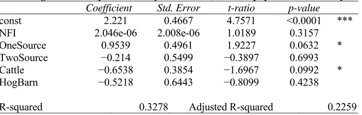
Table 6.2 Regression Output for Carryover Model, Debt Repayment with Carryover

Coefficient Std. Error t-ratio p-value

const 2.221 0.4667 4.7571 <0.0001 ***

NFI 2.046e-06 2.008e-06 1.0189 0.3157

OneSource 0.9539 0.4961 1.9227 0.0632 *

TwoSource −0.214 0.5499 −0.3897 0.6993

Cattle −0.6538 0.3854 −1.6967 0.0992 *

HogBarn −0.5218 0.6443 −0.8099 0.4238

R-squared 0.3278 Adjusted R-squared 0.2259

0 2 4 6 8 10 12 14 1 1.5 2 2.5 3 3.5 More

(31)

25

The net farm income coefficient was positive and explains that for every $10,000 increase in net farm income, the borrower’s debt repayment capacity ratio will increase by 0.02 (Table 6.2). The coefficient for the one source of off-farm income dummy variable was positive, and indicates that if the borrower has one source of off farm income their debt repayment capacity ratio will increase by 0.954. A family that does not have off-farm income could expect their debt coverage ratio to increase by near 1 by taking an off-farm job. A farm that has current off-farm income could expect their debt repayment coverage with ratio to fall by 1 if that off-farm job was lost.

The coefficient for two sources of off-farm income dummy variable was negative, which was not hypothesized. The model suggests that if the operation has two sources of off-farm income, the borrower’s debt repayment capacity will decrease by 0.214. The coefficient for the beef cattle dummy variable was negative, which was not expected. The model explains that if the operation has beef cattle their debt repayment capacity ratio will decrease by 0.654. The coefficient for the hog barn dummy variable was negative, which was not expected. Perhaps the intense capital necessary to build a confinement hog barn has caused this variable to have a negative impact on the borrower’s ability to repay their debt. Although the hog barns can generate a significant income, perhaps the debt service is more demanding than that income. The model explains that if the borrower has a hog barn as part of the operation, their debt repayment capacity ratio will decrease by 0.522.

Table 6.2 and the statistical measures provides an understanding of the strength of the model. The adjusted R-squared value of 0.22 explains that 22% of the variability in debt repayment capacity is explained by the independent variables. This would mean that

(32)

26

approximately 78% of the variability in a borrower’s ability to repay their debt is credited to factors outside of this model.

A review of the statistics explains that two variables in the model were statistically significant at the 90% level, the one source of off-farm income and beef cattle dummy variables.

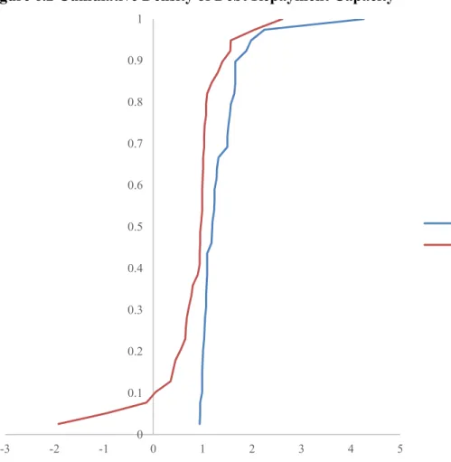
Figure 6.4 Cumulative Density of Debt Repayment Capacity with Carryover

Figure 6.4 displays the cumulative density of debt repayment capacity with carryover of the data set with and without off-farm income. As shown in the graph, when debt repayment capacity with carryover is calculated with off-farm income, only 5% of borrowers are at or below a ratio of 1 (blue line) and nearly 35% of borrowers have a ratio greater than 2. However, when off-farm income is removed as a source of revenue only 30% of borrowers reach the a coverage ratio of 1 (red line) and less than 20% of operations have a ratio over 2. Additionally, when off-farm income is removed approximately 5% of

0 0.1 0.2 0.3 0.4 0.5 0.6 0.7 0.8 0.9 1 -2 -1 0 1 2 3 4 5 6 7 8

DRCC with Off-farm Income DRCC without Off-farm Income

(33)

27

borrowers fall below a debt coverage ratio of zero. This would indicate the operation had such a shortfall of income and working capital that no debt could be serviced and not all operating expenses could be covered. Figure 6.4 illustrates the necessity of off-farm income for nearly all operations in the data to fully meet their debt repayment requirements.

6.4 Summary

The capacity and carryover models were estimated using regression analysis to understand which independent variables had a statistical impact on the dependent variable. The regression model used information collected and calculated during loan reviews and evaluations. Additionally, the model included dummy variables to help better understand the demographics of each borrower and their ability to repay their debt. Regression results from the capacity model yielded rather low adjusted R-squared values that is indicative of debt repayment capacity being explained by factors not present in this model. Regression results from the carryover model yielded slightly better adjusted R-squared values, but were still quite low. The one independent dummy variable that was statistically significant in both models was one source of off-farm income. The significance of that particular variable is understandable. It’s conceivable that an operation with one source of off-farm income and one spouse working full time on the farm is both financially stronger and a more efficient operation. A financially strong and efficient operation would likely be capable of generating cash, and cash is needed to service debt. Additionally, the cumulative density analysis illustrates the importance of off-farm income. Most borrowers in the data set would not be able to repay all their debts without off-farm income.

(34)

28

CHAPTER VII: CONCLUSION & FUTURE ANALYSIS 7.1 Further Analysis

Following the research, data collection, and modeling conducted for this study, it is apparent that there are other areas that can be addressed in future research. The data for this study and the model within it were acquired from one institution’s portfolio. Perhaps a larger, broader set of data would have yielded different results. However, by using data from only one portfolio, the study removes one important variable, the human factor. If the study had gathered data from multiple institutions, the data would have included loans made by various institutions and lenders. Each lender may have different requirements of their borrowers, or may have a higher or lower risk tolerance.

The study determined that the dummy variable for one source of off-farm income was the only statistically significant variable in both models estimated. This was part of the hypothesized outcome, and the hypothesis had hypothesized a positive coefficient for this variable. An operation with a strong outside income source and one spouse working full time on the farm is likely more financially stable and efficient. It can be theorized that an operation that is good at generating revenue and keep costs low has the ability to repay their debts. The generation of cash is a crucial requirement for an operation to repay their debt.

Further research could be conducted to determine if other factors are statistically significant. For example, gross farm income might be statistically significant at certain thresholds. It could be hypothesized that operations with a gross farm income under $100,000 would have a higher debt repayment ratio because they are not relying on that farm income to service debt. Additionally, it could be hypothesized that farms with gross

(35)

29

income over $1,000,000 would have a higher debt repayment capacity because they are larger and may be more stable, and can generate adequate revenue to pay their debts. Operations that fall in the in-between category would be considered medium sized farms and could be trying to expand, or may not have the total revenue necessary to support the farm, family, and their debts.

7.2 Summary and Conclusion

The objective of this thesis was to find if off-farm income positively affected debt repayment capacity enough to keep some operations profitable. Additionally, the thesis was searching to identify other key variables that may impact a borrower’s debt

repayment capacity. Regression analysis was used to identify these key factors. The aim of this research was to examine the hypothesis that certain attributes of a loan borrower directly affects their ability to repay debt. Specifically, it was hypothesized that off-farm income allows operations to repay their debt when farm income alone would not be sufficient for debt coverage. In conclusion, the hypothesis was not rejected and it was determined that a borrower’s ability to repay their debt can be affected by off-farm income.

This study contains findings that will assist ABC Bank and Trust in the future when making decisions on accounts with clients in their current portfolio and when evaluating potential borrowers. Off-farm income substaintially improves the coverage ratios and conversely, if that off-farm job is lost, the ability to repay debt is affected substantially. Responsible lending, based on a borrower’s ability to repay their debt, is absolutely vital to a successful lending institution. This study should provide

(36)

30

decisions on how much exposure they would be willing to incur with a certain borrower. Other financial information should be used when making a final lending decision such as tax returns, current ratios, and debt-to-equity, among others. This study is not an all-encompassing decision making tool, but rather an additional tool for a lending institution to evaluate their portfolio.

The discoveries of this model suggest there are many variables that affect a borrower’s ability to service their debt. A low R-squared model value was found as a result of the regression analysis of the models. This indicated that the independent variables within the models explained the dependent variable to some extent, but there are many other factors not available in this data. In closing, the key factors used in the model contribute to the borrower’s ability to repay their debt, but cannot accurately predict the borrower’s debt repayment capacity.

(37)

31

REFERENCES

Adonizio, Kook, and Royales. 2012. Impact of the drought on corn exports: paying the price. U.S. Bureau of Labor Statistics.

Briggeman, Brian C. 2011. "The Importance of Off-Farm Income to Servicing Farm Debt."

Federal Reserve Bank of Kansas City.

Dobbs, Kevin. 2016. "Farm income is the lowest since 2002. Here's why you should care."

Deseret News, July 11.

Fernandez-Cornejo, Jorge. 2007. "Off-Farm Income, Production Decisions, and Farm Economic Performance." https://naldc.nal.usda.gov/catalog/20582.

Gretl. 2017. January 15.

Jette-Nantel, Simon. 2013. Implications of Off-Farm Income for Farm Income Stabilization Policies. PhD Thesis, University of Kentucky.

McMillan, Tracie. 2016. "Farmers Work a Second Shift to Supplement Income." National Geographic, February 25.

Prager, Daniel. 2016. United States Department of Agriculture. December 21. Accessed

January 15, 2017. https://www.ers.usda.gov/topics/farm-economy/farm-household-well-being/health-insurance-coverage/.

USDA. 2015. "ARMS Farm Financial and Crop Production Practices."

https://www.ers.usda.gov/data-products/arms-farm-financial-and-crop-production-practices/.

Zwilling, Krapf, and Raab. 2016. "How Will Family Living Affect My 2017 Budgets."

Off-farm income: evaluating the effects of off-farm income on debt repayment capacity