Evaluating Alternative Safety Net Programs in Alberta: A Firm-level Simulation Analysis
Scott R. Jeffrey and Frank S. Novak Staff Paper 99-03
Department of Rural Economy
Faculty of Agriculture, Forestry and Home Economics
University of Alberta Edmonton, Canada
R
URAL
E
CONOMY
Evaluating Alternative Safety Net Programs in Alberta: A Firm-level Simulation Analysis
Scott R. Jeffrey and Frank S. Novak Staff Paper 99-03
Scott Jeffrey is Associate Professor, Department of Rural Economy. Frank Novak was formerly, Associate Professor, Department of Rural Economy and is presently, Managing Director, Alberta Pig Company.
The financial support of AARI and SSHRC for this project is gratefully acknowledged.
The purpose of the Rural Economy “Staff Papers” series is to provide a forum to accelerate the presentation of issues, concepts, ideas and research results within the academic and professional community. Staff Papers are published without peer review.
EVALUATING ALTERNATIVE SAFETY NET PROGRAMS IN ALBERTA: A FIRM-LEVEL SIMULATION ANALYSIS
Scott R. Jeffrey and Frank S. Novak
Department of Rural Economy, University of Alberta Edmonton, Alberta, Canada
ABSTRACT
This paper examines alternative risk management strategies in terms of their effectiveness for three representative Alberta farm operations. Stochastic dynamic simulation methods are used to model financial performance for these farms, and alternative risk management programs are compared in terms of their ability to stabilize returns, support income and reduce the probability of bankruptcy. The results suggest that government programs such as the Net Income
Stabilization Account (NISA) program or the Farm Income Disaster Program (FIDP) in Alberta have some benefits in terms of supporting income levels and reducing the chances of farm failure. Neither program is very effective, however, in stabilizing year to year income or cash flow for the farm operations. As a risk management program, FIDP is more effective than NISA but this improved performance comes at the price of higher government costs. Performance of NISA and FIDP, relative to alternative risk management programs and strategies such as forward contracting or crop insurance, is mixed. In some cases, NISA does not seem to provide benefits beyond those available from other strategies, while FIDP tends to perform better than the alternatives. Finally, while increased debt load weakens firm financial performance, NISA and FIDP still provide some benefits in terms of supporting income and reducing the probability of bankruptcy.
INTRODUCTION
Canadian agriculture has a long history of government involvement in programs designed to stabilize prices and incomes. These programs have come under renewed scrutiny due to the combined effects of government budget constraints and international trade negotiations. The result has been a move from commodity specific and price based programs towards programs that are intended to stabilize farm gross margin1 or net income. These are often referred to as safety
net programs. This fundamental policy reform is consistent with shifts in attitudes concerning government intervention in agriculture (Agriculture Canada 1989).
In Alberta, two public safety net programs currently available to agricultural producers are the Net Income Stabilization Account (NISA) program and the Farm Income Disaster Program (FIDP). While the two programs differ in terms of the rules governing program “mechanics”,
each is intended to stabilize producer returns. There is currently little information on the potential effectiveness of NISA or FIDP in stabilizing income or improving financial performance (e.g., wealth enhancement).2 It is also unknown whether either of these programs is any more effective
than alternative risk management or stabilization strategies available to Alberta farmers. Given the importance of risk and risk management in agriculture, and the long term implications of NISA and FIDP in terms of the potential cost to taxpayers, these are important issues.
The objectives of this paper are to a) evaluate NISA and FIDP in terms of their ability to stabilize returns or otherwise improve financial performance over time for different types of farming operations in Alberta; and b) compare the two programs to alternative risk management programs and strategies currently available to Alberta farmers. The “effectiveness” of any particular
program or strategy is evaluated on the basis of three criteria; the ability to stabilize returns over time, the ability to improve financial performance, and the ability to reduce the risk of business failure (i.e., bankruptcy).
These objectives are achieved through the use of dynamic stochastic simulation for representative Alberta farm operations. Participation in NISA and FIDP is evaluated, relative to
non-participation, using three criteria; ending wealth levels, the ability to support and stabilize income and cash flow over the relevant time horizon, and the probability of bankruptcy. In addition, alternative risk management strategies are modelled for the representative farms. These alternatives are evaluated using the same three criteria.
SAFETY NET PROGRAMS
The term safety net is used to describe public programs that are intended to support and/or stabilize producer incomes. NISA is an example of a safety net program. Two other safety net programs are also considered in this paper; the Farm Income Disaster Program (FIDP) and crop insurance. A brief description of these three programs is provided below.
The Net Income Stabilization Account (NISA) program is a voluntary program jointly
administered by the federal and provincial governments. The objective of NISA is to provide a mechanism by which participating agricultural producers may stabilize revenues over time. As currently structured, NISA is essentially a savings account. Farmers make contributions in years of high income and draw from their account in low income years, based on certain program triggers.
Producers may contribute up to 20 percent of net sales into a program account each year. Net sales are total farm sales minus purchases of all agricultural products, and represent the net value of agricultural production for the farm operation. The federal and provincial governments match farmer contributions up to a level of three percent of net sales. Unused non-matching eligible deposits may be carried forward by the farmer. Interest is paid on the program account at a rate consistent with market interest rates. Farmer contributions earn a three percent bonus as well. There are dollar value limits placed on annual contributions and account balances.
NISA withdrawals are “triggered” by shortfalls in either of two performance measures. If gross margin for the farm falls below the five-year historical average, the farmer may withdraw an amount up to the difference between the two values. If net income for the farm falls below $10,000, the farmer may withdraw an amount up to the difference between the two values. Gross margin is equal to net sales minus eligible expenses (i.e., most farm expenses excluding interest, depreciation, lease or rental payments, and improvement costs). Net income is equal to net sales minus operating and fixed costs for the farm operation (i.e., before-tax profit). The farmer may withdraw the larger of the two amounts indicated by the triggers. The withdrawal may not exceed the NISA program account balance.
Farm Income Disaster Program (FIDP)4
FIDP is a voluntary support program initiated and funded by the Alberta provincial government. The objective of FIDP is to lessen extreme income reductions occurring because of circumstances that are beyond the control of the producer. The mechanics of the program are relatively simple.
In any given year, an application for a program payment may be made if the producer’s program margin is less than 70 percent of his/her average program margin for the previous three years. The payment is equal to the difference between these two values. The program margin for FIDP calculations is basically the same as gross margin for NISA; that is, net sales minus the same eligible expenses. If the program margin is negative, the payment will be equal to the 70 percent of the three year historical average value; that is, there is no support for negative program margins. The program caps annual payments at $100,000 per individual or $500,000 per
corporation. Finally, FIDP payments are reduced by the amount of any government contributions to producers’ NISA accounts.
Crop Insurance
Crop insurance is a well-established risk management tool for crop producers. Typically, crop insurance is a voluntary program designed to provide some protection against yield risk for crop producers. In Alberta, crop insurance is jointly funded by participating producers (50 percent) and the provincial (25 percent) and federal (25 percent) governments. The producers’
contributions arise from premiums paid for insurance coverage.
Producers enrol in crop insurance by paying a per acre premium. This premium varies by crop and by risk area. Crop insurance risk areas are determined by climate, soil type, etc. The
insurance coverage received by the producer is equal to 70 percent of the long-term area yield for the specific crop, adjusted by a factor that reflects the producer’s average yields relative to the area average. If the actual crop yield obtained by the producer is below the coverage level, a crop insurance payment is generated. The payment is equal to the yield shortfall (i.e., coverage level minus actual yield) multiplied by the relevant crop price.
METHODOLOGY
The methodology used for this study consists of three parts; identification of representative farms, simulation procedures, and risk management program analysis. Representative firm analysis is used to model the effectiveness of alternative risk management options and programs for Alberta
farm operations. Three representative farms are defined for this purpose; a beef feedlot, a cropping operation and a farrow-to-finish hog operation. The financial performance for each of these farming operations, assuming different risk management scenarios, is modelled using stochastic, dynamic simulation procedures. The results from the simulation analysis are then examined in order to evaluate the risk management options. Each of these aspects is discussed in more detail below.
Representative Farms
The three representative farms (i.e., beef, crop and hog) defined and used in the simulation
analysis are not intended to be “average” farms. Instead, they are representative in that they could be considered as being “typical” of many commercial farm operations in Alberta. For each farm, production and technical characteristics are developed using historical data. These characteristics include capital structure (i.e., dollar values for land, buildings, equipment, etc.), production levels and patterns (e.g., crop acreage and yields), costs and returns for the different enterprises (e.g., feed costs, machinery expenses, output prices, crop yields), as well as marketing patterns.
The beef operation is a feedlot that markets 5000 head of cattle per year. There are no crop enterprises and all inputs are purchased including cattle and feed. The feedlot operator utilizes seasonal marketing, with one-half of the animals being marketed in June and July and the other half being marketed in the period from November to January. The asset base for this operation (i.e., land, buildings and equipment) is approximately $950,000. Data used to develop the production and financial characteristics for this farm operation are obtained from Novak and Viney (1995).
The cropping operation is a 1600 acre farm that is located near Trochu, Alberta. The farm makes use of conventional tillage systems, and has a crop rotation of wheat-barley-canola. The asset base for this operation (i.e., land, buildings and equipment) is approximately $1,285,000. Data used to develop the production and financial characteristics for this farm operation are obtained from Bauer et al (1995).
The hog farm is a farrow-to-finish operation with 350 sows. The farm does not have any crop enterprises and purchases all feed and breeding stock replacements. The operation utilizes a uniform marketing strategy, marketing 132 pigs per week. The asset base for this operation (i.e., land, buildings, equipment and breeding stock) is approximately $1,200,000. Data used to
develop the production and financial characteristics for this farm operation are obtained from Bresee (1997).
Rather than assume a particular debt level for the farms, the simulation analysis is carried out for two alternative debt scenarios. This provides an opportunity to examine the effects of debt level (i.e., financial risk) on the effectiveness of alternative risk management strategies. In each case, the debt scenario is characterized by a particular debt-to-asset ratio (i.e., D/A). Low debt is represented by a D/A of 0.25 and high debt is represented by a D/A of 0.50.5 The particular D/A
ratio is then multiplied by total assets for the farm to obtain the initial debt level.
Simulation Analysis
The representative farms are modelled using multi-period stochastic simulation. Each
combination of representative farm, debt level and risk management option is simulated over a ten year time horizon. The simulation is stochastic in that 5000 iterations are used for each
combination. Annual costs and returns are drawn from specified probability distributions, which are based on historical data (same sources as for representative farm characteristics). The only exception for this is the crop farm for which crop yields and prices, rather than gross revenue, are drawn from separate distributions. This is done due to the necessity of being able to identify crop yields for the purposes of modelling participation in crop insurance.
The simulation model itself is basically a set of accounting equations. The model calculates annual sales and expenses, debt servicing requirements, depreciation, etc. It tracks income and cash flow measures, and calculates ending financial position (i.e., ending wealth) on a year by year basis. The model also incorporates the possibility of financial failure, as the farm operation is declared bankrupt if ending wealth becomes negative at any point in the simulation. Finally,
depending on the particular risk management scenario, the model includes calculations for variables such as program margins, contributions/withdrawals for NISA accounts, FIDP payments, crop insurance payouts, etc. The model is programmed using GAUSS (Aptech Systems Inc. 1996).
Risk Management Alternatives: Identification and Assessment
For each representative farm/debt level combination, alternative risk management options or strategies are modelled. The default scenario in each case is non-participation in any risk management program or strategy, referred to as the BASE scenario. Participation in the NISA program is the NISA scenario. It is assumed that producers make the maximum matchable NISA contribution in each year (i.e., two percent of net sales), even if borrowing is necessary to obtain the funds.6 Participation in the provincial FIDP program is referred to as the FIDP scenario.
Finally, a “combination scenario” is modelled for each farm, involving participation in both NISA and FIDP. This is referred to as the BOTH scenario.
An additional risk management strategy is modelled for the beef farm and the cropping operation. This is done to assess the performance of NISA and FIDP relative to alternative strategies
currently available to producers. The particular alternative varies by farm, as discussed below. This is done for two reasons. First, different types of farm operations have access to different types of risk management strategies, depending on the particular enterprise. Secondly, each of the alternatives affects the farm-level distributions for returns in somewhat unique ways, making a more interesting and complete comparison with NISA and FIDP.
For the beef farm, the alternative modelled is the use of selective forward contracting for the cattle. If the terms are favourable the producer will utilize forward contracting to reduce price risk. Details for this scenario are provided by Novak and Viney (1995). The scenario, referred to as CONTRACT, has the effect of reducing the mean and variability for the producer’s net sales.7
For the cropping operation, the alternative strategy is participation in crop insurance. It is assumed that the producer insures all acres of all three crops. As discussed earlier, in return for paying a per acre premium, the producer receives a certain yield guarantee (i.e., 70 percent of the adjusted long-term area yield). Within the simulation analysis this scenario, referred to as
INSURE, has the effect of truncating the yield distributions at the coverage level.
The alternative risk management strategies identified above are compared and evaluated in terms of their “effectiveness”. Three criteria are used to measure effectiveness. First, the strategies are assessed in terms of their ability to stabilize returns over time. Stability refers to the ability to reduce variability for a particular measure. In this case, stability is measured in terms of income and cash flow. Average values and variability for net income and net cash flow are measured on an annual basis. From these, statistical confidence intervals are calculated and compared between alternative strategies.
Effectiveness is also measured in terms of the ability to support income; that is, improve financial performance. The ability of a strategy to “support” income can be measured using net income. Alternatively, ending wealth also incorporates profit levels. Higher net income levels result in higher ending wealth levels. Therefore, average ending wealth is used to compare strategies in this respect. Average ending wealth is the farm’s equity position after ten years, averaged over all iterations.8
Improved financial performance can also be measured in terms of liquidity; that is, the ability to support cash flow. Cash flow support is measured by the probability of illiquidity. This
probability is calculated as the proportion of solvent years over the 5000 iterations that have a negative net cash flow. If one strategy supports cash flow to a greater extent, it might be expected that the probability of illiquidity would be lower for that strategy.9
The third criterion is the ability to reduce the risk of business failure. Each strategy is assessed with respect to the probability of bankruptcy. The probability of bankruptcy represents the proportion of the 5000 iterations ending in bankruptcy, expressed as a percentage.
RESULTS AND DISCUSSION
Tables 1, 2 and 3 provide a summary of the simulation results for the three representative farms and the various risk management scenarios. From these tables, some general trends are identified and discussed below.
Effectiveness of NISA and FIDP versus Non-Participation (BASE)
One criterion used to evaluate the safety net programs is the degree to which they stabilize income and net cash flows. This may be done by examining the impact of NISA and FIDP on the
variability of these measures over time, relative to the BASE scenario. If NISA and FIDP are effective in stabilizing income and cash flow, it is expected that the degree of year-to-year
variability will be reduced. For each farm and each risk management alternative, 95% confidence intervals are calculated for net cash flow and net income. These statistical confidence intervals around average values over time are compared between the alternative scenarios. If NISA and FIDP are effective in stabilizing returns, the confidence intervals should be “narrower”; that is, the year-to-year variability should be reduced.
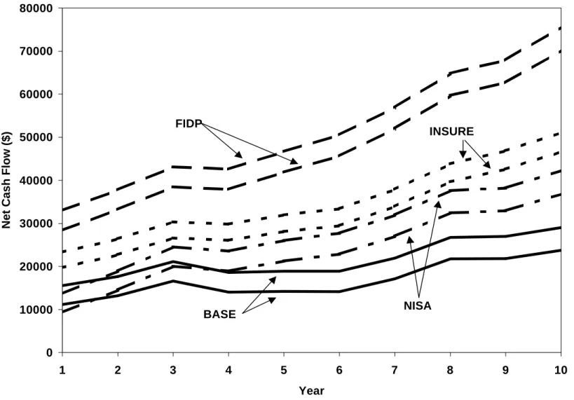
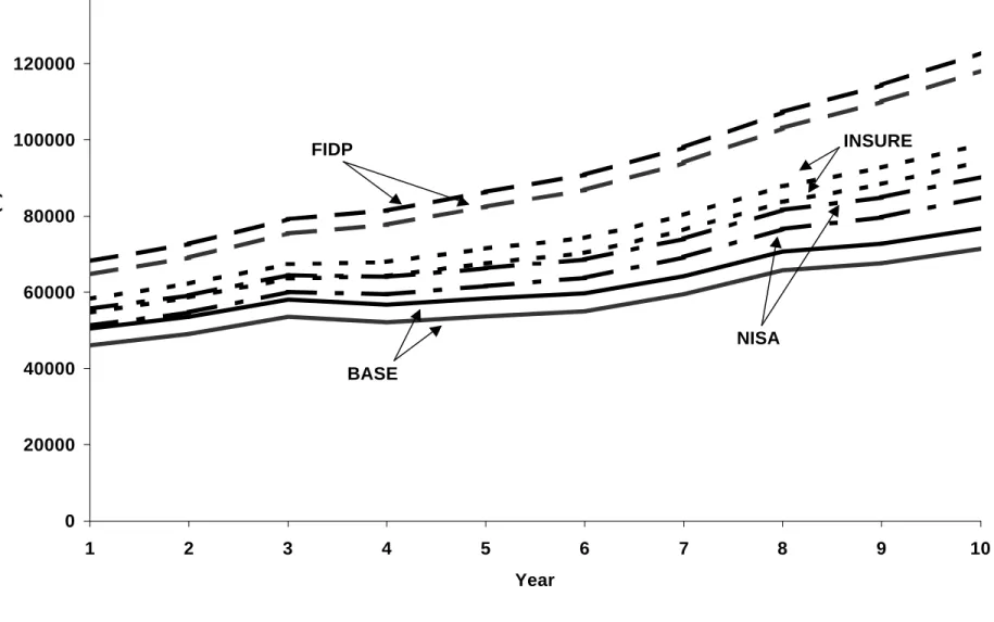
For space reasons, not all confidence intervals are provided here. However, Figures 1 and 2 provide the 95% statistical confidence intervals for the low debt version of the cropping operation. The patterns exhibited in these figures are consistent with those for the other
representative operations. Therefore, they will be used to illustrate the effectiveness of the safety net programs in terms of stabilization.
As shown in Figure 1, NISA and FIDP have little impact on the stability of net cash flow. Specifically, the “width” of the confidence intervals does not differ between the various risk
management alternatives. In contrast, Figure 2 suggests that NISA and FIDP have some stabilizing effects on net income (i.e., the confidence interval around the average value is reduced), although the impact is slight.
Much of the difference in the ability of the two programs to support and stabilize income versus cash flow is due to the timing of withdrawals or payments from these programs. Payments from NISA or FIDP are received in the calendar year following the year in which the shortfall occurs, due to the fact that the calculations are based on tax filer information. While the accrual basis on which net income is calculated results in FIDP payments, for example, being allocated to the production year on which they are based, this is not the case with net cash flow. Thus,
participation in the programs (particularly FIDP) does result in slightly improved income stability, but not cash flow stability.
Another criterion used to evaluate NISA and FIDP is the degree to which they support income and cash flows for the farms. Average ending wealth provides an indication of this with respect to income. Given the method of asset valuation used in the simulation analysis (i.e., cost-based), wealth only increases if the business generates positive profits. As can be seen from the tabular results, both NISA and FIDP result in increased wealth levels, suggesting that net income levels are increased as well. Depending on the farm and debt level, NISA provides an improvement of between 7 and 94 percent, while the corresponding range of improvement attributable to FIDP is 24 to 105 percent. This pattern is echoed in Figure 2, as the 95 percent confidence intervals for net income associated with NISA and FIDP are consistently at a higher level than is the case for the BASE scenario.
In assessing liquidity performance, the probability of illiquidity is used; that is, the proportion of solvent years in which net cash flow is negative. If net cash flows are supported and improved by these programs, the probability of illiquidity should decrease. This is true, to a certain extent. Participation in NISA or FIDP consistently results in a lower probability, although the
improvement is not always significant. It would seem, then, that the safety net programs are more effective in supporting income than cash flows.
The ability of NISA and FIDP to support and improve financial performance for the
representative operations is primarily related to the subsidization aspects of each program. If a farmer participates in FIDP, payments represent a direct transfer from the provincial government to the producer. With participation in NISA, a farmer’s contributions are matched (to a degree) by the federal and provincial governments. There is also an interest bonus paid on farmer
contributions. Thus, the ability of producers to draw on their NISA accounts is based not only on their own contributions but also on a transfer of funds from governments.
The final criterion used in assessing the effectiveness of the safety net programs is the ability to reduce the chances of business failure; that is, the probability of bankruptcy. Both NISA and FIDP reduce the probability of bankruptcy for the farms. This is consistent across farms and debt levels. In many cases, the improvement is significant (i.e., between 19 and 76 percent reduction for NISA, and between 59 and 100 percent reduction for FIDP). As well, both NISA and FIDP improve the average ending wealth levels for the farms and reduce the relative variability (i.e., the coefficient of variation), when compared with the BASE scenario. Thus, the safety net programs are effective in reducing the chances of business failure. Again, this improvement is largely attributable to the direct transfer of funds from provincial and/or federal governments to the farmers through the mechanics of the two programs.
A Comparison of NISA and FIDP
The two safety net programs may be compared to each other, using the same three criteria
discussed earlier. If this is done, in general it may be said that FIDP is more effective than NISA. There is little difference in the “width” of the net income and net cash flow confidence intervals (see Figures 1 and 2), suggesting that the two programs are similar in their ability (or lack thereof) to stabilize returns over time. However, the confidence intervals associated with FIDP are higher
than those for NISA. This suggests that FIDP is the superior program in terms of supporting income. This is confirmed through a comparison of average ending wealth levels for the two programs. FIDP consistently results in higher average ending wealth. Finally, FIDP also results in lower probabilities of bankruptcy, suggesting that it does a better job of improving the chances of firm survival. These trends are consistent across farms and debt levels.
The difference in performance may be largely attributed to the mechanics of the two programs. In order to be effective, NISA requires the farmer to contribute funds to the program account. Withdrawals are limited both by the triggers and by the account balance. Assuming that the farmer always makes the maximum matchable contribution, this contribution decision rule can also actually exacerbate cash flow problems already existing within the farm operation. In contrast, FIDP requires no equivalent contributions as the program is completely funded by the provincial government.10
The superior performance of FIDP comes at a cost. As noted in Tables 1 to 3, the average annual government contribution to FIDP (i.e., government payments) is greater than the corresponding government “cost” for NISA (i.e., matching contributions to accounts plus bonus interest payments). In addition, as the relative degree of improvement for FIDP as compared to NISA increases, so does the difference in government cost. Evidence of this is provided by noting that the superiority of FIDP over NISA is more pronounced for the beef and hog operations where, correspondingly, the difference in annual government contributions between the two programs for these farms is greater.
As noted in the discussion of methodology, a combination risk management scenario is modelled for each farm. This combines participation in both NISA and FIDP and is referred to as the BOTH scenario in Tables 1 to 3. As might be expected, the use of both NISA and FIDP improves financial performance to an even greater extent relative to participation in either program alone. This is particularly true with respect to support for income (i.e., ending wealth levels)and the probability of financial failure (i.e., probability of bankruptcy). Variability of ending
wealth is also reduced to a greater extent, when compared to the BASE scenario. This suggests that there is some degree of complementarity between the programs. However, even the
combined programs do not provide significant benefits in terms of stabilizing income or cash flows. Once again, the improved performance comes at an increased government cost, relative to participation in either of the programs in isolation.
NISA and FIDP versus Risk Management Alternatives
Two alternative risk management programs are modelled; selective contracting for the beef operation (CONTRACT) and crop insurance for the cropping operation (INSURE). The details and impacts of these options are discussed earlier in the paper.
The performance of the alternative risk management strategies for the farms is mixed. The selective contracting (CONTRACT) strategy for the beef feedlot does not provide significant benefits relative to the BASE scenario. Average ending wealth levels are improved slightly, relative to the BASE scenario. Bankruptcy rates are reduced slightly, while the probability of illiquidity actually increases relative to the BASE. Relative to either NISA or FIDP, the CONTRACT strategy does not perform well with respect to any of the three criteria. Overall, then, this particular risk management strategy provides poor protection relative to the public safety net programs.
The crop insurance strategy (INSURE) for the cropping operation provides more significant benefits and is somewhat effective in managing risk. For example, from the results in Table 2 the improvement in average ending wealth relative to the BASE scenario varies from 11 percent (low debt) to 22 percent (high debt). Probability of bankruptcy and illiquidity also improve relative to the BASE. If compared to NISA, crop insurance is as effective or more effective when
considering the various criteria outlined earlier. This may be seen by comparing ending wealth, and probabilities of bankruptcy and illiquidity. In contrast, FIDP provides superior performance when compared to crop insurance (INSURE).
Consistent with the previous discussion, the differences in performance are attributable to differences in the mechanics of the various programs. While farmers are required to pay a premium to gain access to insurance payouts (if warranted), there is no limit on payouts. This is in contrast to NISA, where again withdrawals are limited by producers’ account balances. If compared to FIDP, crop insurance does not perform as well at least in part because of the difference in the risks being managed. While FIDP is designed to limit exposure to gross margin risk, crop insurance limits exposure to only yield risk.
Also consistent with previous discussion, the effectiveness of the programs is directly related to the level of government cost. As noted in Table 2, on an annual average basis crop insurance is less costly than FIDP, but more costly than NISA. This corresponds to the general relationship in terms of their ability to manage risk. Here, government contributions for crop insurance are calculated as 50 percent of the average annual payout from the program to be consistent with the government share of crop insurance premiums, and assuming actuarial soundness for the program.
Impact of Debt Levels
The results in Tables 1, 2 and 3 allow for an examination of the impact on the effectiveness of risk management strategies of debt levels. Not surprisingly, financial performance for any particular scenario deteriorates with increased debt. With an increased drain on cash flow and income due to principal and interest payments on debt, average ending wealth for all farms decreases relative to the low debt scenario. In addition, the probabilities of bankruptcy and illiquidity for all farms increase, in some cases significantly.
The impact of increased debt on the effectiveness of the risk management strategies is mixed. The relative improvement in the probability of bankruptcy attributable to participation in NISA or FIDP decreases with increased debt levels. For example, participation in NISA for the low debt beef feedlot (Table 1) reduces the probability of bankruptcy by 55 percent (i.e., from 28.5 percent to 12.8 percent). For the same farm with high debt, the reduction attributable to NISA is only 43
percent (i.e., from 48.7 percent to 27.8 percent). This pattern is consistent for all farms and all NISA/FIDP scenarios. The same pattern also exists for the probability of illiquidity.
The effect of debt level on the relative improvement in ending wealth levels is also consistent across programs. In general, the ability of NISA or FIDP to improve ending wealth (i.e., support income levels) is not adversely affected by debt levels. For example, participation in NISA by the low debt beef feedlot (Table 1) results in a 65 percent increase in average ending wealth (i.e., from $929,093 to $1,537,096). For the same farm with high debt, the improvement is 94 percent (i.e., from $521,524 to $1,012,283). Similar patterns exist for the various representative farms, for participation in FIDP.
This consistency is interesting, given the differences between NISA and FIDP in program objectives and mechanics. FIDP is not intended to address variability in returns due to debt servicing requirements. As a result, the payment “trigger” is based on program margin
calculations which do not include interest costs. In the case of NISA, there are two withdrawal “triggers”, one of which is based on net income which includes debt servicing costs. This allows some support for producers with higher debt servicing costs. However, the evidence suggests that despite these differences, both programs are able to provide support regardless of debt level.
One other point may be made with respect to debt levels. To a certain extent, program participation (i.e., NISA, FIDP or BOTH scenarios) allows producers to increase debt levels while maintaining a certain level of risk exposure. Using the beef feedlot as an example (Table 1), the probability of bankruptcy for the low debt farm and no risk management strategy is
approximately 29 percent. If the debt level is increased to “high” (i.e., debt-to-asset ratio
increased from 0.25 to 0.50), participation in NISA results in the probability of bankruptcy being virtually unchanged (i.e., approximately 28 percent). This has implications for agricultural producers who are considering expansion strategies where a significant amount of the financing will come from debt sources.
CONCLUDING COMMENTS
The effectiveness of NISA as a risk management program is mixed. The version of NISA
examined in this paper is somewhat effective in supporting net income for participating producers. It is also effective in reducing the chances of financial failure. However, NISA is not very
effective in supporting or stabilizing cash flows for the farm operation, largely due to the time lag between when shortfalls occur and when withdrawals are made available. While increased debt levels weaken performance both with and without participation in NISA, the ability of NISA to improve performance and decrease the probability of bankruptcy is unchanged.
The FIDP program implemented by the provincial government in Alberta is more effective than NISA in managing risk; that is, reducing the chances of financial failure and increased support for income. However, this effectiveness comes at a greater program cost to the government. As well, FIDP has the same shortcomings as NISA in terms of a lack of effectiveness in stabilization of income and cash flow. As is the case with NISA, FIDP is also able to maintain some risk management benefits under higher debt levels, despite the fact that the program is not intended to manage financial risk resulting from debt financing decisions.
If compared to alternative risk management strategies (e.g., selective contracting or crop insurance), the performance of NISA is mixed. It would appear that, to a certain extent, agricultural producers already have access to risk management strategies that may provide the same level of protection from risk. However, it is also evident that NISA does provide some advantages for certain groups of producers. FIDP is clearly a superior program, from a
producer’s perspective, in terms of managing risk associated with revenue and gross margin, as evidenced by the comparisons made for the beef feedlot operation (i.e., versus selective
contracting) and the cropping operation (i.e., versus crop insurance).
Overall, it may be concluded that both NISA and FIDP are somewhat effective programs, given their objectives. Both provide long terms stability to producers, largely due to a transfer of funds from taxpayers. Both programs are also somewhat effective relative to at least some of the risk
management alternatives available to producers. However, neither program provides much stability in net income or net cash flow on a year-to-year basis.
One last point that may be made is that there is a significant public cost associated with both NISA and FIDP. This is particularly true for FIDP, where there are no farmer contributions required as compared to NISA. This is an important consideration, particularly when assessing the comparisons made with other risk management options. A question left unanswered by this analysis is that of the optimal tradeoff between government (i.e., taxpayer) cost and risk
1. Gross margin refers to the margin between revenue and variable expenses. For the purposes of the safety net programs examined in this paper, the term program margin is also used.
2. There has been some research conducted with respect to NISA, primarily relating to agriculture in Saskatchewan. Spriggs and Taylor (1995) examine the effects of NISA on Saskatchewan grain farms. As well, Spriggs et al (1995) examine the aggregate effects of NISA for the Saskatchewan agricultural sector. Finally, Spriggs and Nelson (1997) examine the impact of an enhanced NISA program in Saskatchewan.
3. Details concerning the structure and operation of NISA are provided by Agriculture and Agri-Food Canada (1999).
4. The discussion of the mechanics for FIDP and crop insurance in Alberta is based on information from Block (1996).
5. In this study, a third debt level is also considered, with an initial D/A of 0.75. The simulation results for this debt scenario are not reported here, but are available from the authors upon request.
6. This represents one possible “decision rule” for NISA contribution decisions. Other decision rules are modelled in this study, including making contribution decisions based on net cash flow or operating balance (i.e., chequing account balance) considerations. The simulation results based on these decision rules are not reported here but are available from the authors.
7. A similar risk management strategy is also modelled for the hog operation. The results and relative effectiveness are similar to those for the selective contracting strategy for the beef feedlot. As a result, the results for the hog operation are not presented here.
8. Ending wealth for any iteration resulting in bankruptcy is set to zero.
9. The interpretation of this measure is limited by the use of an annual model; that is, an important facet of liquidity is the availability of cash through the year as needed. This aspect, which is particularly significant for beef and hog operations that use uniform marketing strategies, is ignored here. However this measure does indicate, on an annual basis, whether or not the farm operation was sufficiently liquid.
10. As noted earlier, the actual version of FIDP implemented in Alberta includes a cap on annual payments for individual operations. This cap would potentially affect “larger” farm operations, and is not incorporated into this analysis. However, the effective cap for a specific operation depends on the ownership structure, and can vary from $100,000 to $500,000. Since no particular ownership structure is specified for any of these operations,
it is difficult to assess the potential impact of the annual payment cap. The simulation results for the representative farms suggest that, while the maximum single annual payout from FIDP exceeds $100,000 for all farms, in no instance is it as great as $500,000.
REFERENCES
Agriculture and Agri-Food Canada. 1999. Net Income Stabilization Account (NISA). http://aceis.agr.ca/nisa/n9608e.html
Agriculture Canada. 1989. Growing Together: A Vision for Canada’s Agri-Food Industry.” Ottawa.
Aptech Systems, Inc. 1996. GAUSS Mathematical and Statistical System. Maple Valley WA:Aptech Systems, Inc.
Bauer, L., S.R. Jeffrey and C.C. Orlick. 1995. “A Comparison of Risk between Continuous and Fallow Cropping Regimes.” Project Report No. 95-08. Final Report for Alberta
Agricultural Research Institute Project No. 04-0492. Department of Rural Economy, University of Alberta. December.
Block, R. 1996. An Examination of Risk: An Application of Agricultural Public Risk Programs. Unpublished M.Ag. Project Report, Department of Rural Economy, University of Alberta. March.
Bresee, D. 1996. New Derivative Instruments for Alberta Hog Producers. Unpublished M.Sc. Thesis, Department of Rural Economy, University of Alberta. February.
Novak, F.S. and B. Viney. 1995. Alternative Pricing and Delivery Strategies for Alberta Cattle Feeders. AARI Project Report 95-06. Department of Rural Economy, University of Alberta.
Spriggs, J. and T. Nelson. 1997. Effects of Enhancing NISA on Income Stabilization and Support. Canadian Journal of Agricultural Economics 45 (2): 123-9.
Spriggs, J. and J.S. Taylor. 1995. An Analysis of Alternative Income Safety Nets for Saskatchewan Grain Farms. Final Report submitted to Policy Branch, Agriculture Canada. January.
Spriggs, J., J.S. Taylor, S. Hosseini, H. McLennan and D. Niekamp. 1995. Aggregate Impacts of a Value-Added Income Stabilization Account. Final Report submitted to The
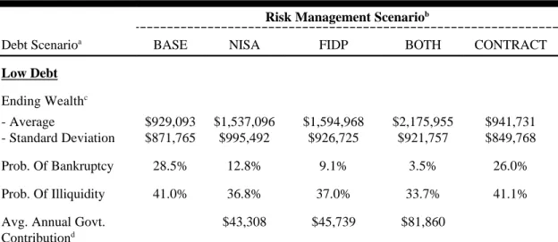
Table 1: Simulation Results for the Beef Feedlot
Risk Management Scenariob
Debt Scenarioa
BASE NISA FIDP BOTH CONTRACT
Low Debt Ending Wealthc - Average $929,093 $1,537,096 $1,594,968 $2,175,955 $941,731 - Standard Deviation $871,765 $995,492 $926,725 $921,757 $849,768 Prob. Of Bankruptcy 28.5% 12.8% 9.1% 3.5% 26.0% Prob. Of Illiquidity 41.0% 36.8% 37.0% 33.7% 41.1%
Avg. Annual Govt. Contributiond $43,308 $45,739 $81,860 Medium Debt Ending Wealthc - Average $521,524 $1,012,283 $1,069,425 $1,613,669 $524,666 - Standard Deviation $683,106 $879,718 $815,389 $860,106 $675,647 Prob. Of Bankruptcy 48.7% 27.8% 20.0% 8.7% 47.7% Prob. Of Illiquidity 42.7% 39.5% 39.5% 36.6% 43.5%
Avg. Annual Govt. Contributiond
$43,484 $46,473 $81,948
a
The two debt scenarios are based on initial debt levels, with low representing D/A=0.25 and high representing D/A=0.50.
b The various risk management scenarios are as defined in the main body of the paper. c Statistics for ending wealth are based on all 5000 iterations, with bankruptcy being
represented by zero ending wealth.
d
Government contributions for NISA include matching contributions and interest rate bonus. For FIDP, government contributions are the payments made to producers.
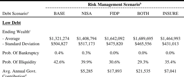
Table 2: Simulation Results for the Cropping Operation
Risk Management Scenariob
Debt Scenarioa
BASE NISA FIDP BOTH INSURE
Low Debt Ending Wealthc - Average $1,321,274 $1,408,794 $1,642,092 $1,689,695 $1,464,993 - Standard Deviation $504,827 $517,173 $475,820 $465,556 $431,013 Prob. Of Bankruptcy 0.4% 0.3% 0.0% 0.0% 0.0% Prob. Of Illiquidity 42.6% 39.9% 30.6% 29.3% 35.4%
Avg. Annual Govt. Contributiond $5,285 $17,893 $21,535 $7,041 Medium Debt Ending Wealthc - Average $513,859 $591,987 $810,192 $856,767 $628,085 - Standard Deviation $453,474 $480,435 $478,042 $472,197 $429,250 Prob. Of Bankruptcy 20.0% 16.2% 5.5% 3.9% 9.2% Prob. Of Illiquidity 70.1% 67.5% 58.4% 56.8% 69.9%
Avg. Annual Govt. Contributiond
$5,280 $17,872 $21,520 $7,010
a
The two debt scenarios are based on initial debt levels, with low representing D/A=0.25 and high representing D/A=0.50.
b The various risk management scenarios are as defined in the main body of the paper. c Statistics for ending wealth are based on all 5000 iterations, with bankruptcy being
represented by zero ending wealth.
d
Government contributions for NISA include matching contributions and interest rate bonus. For FIDP, government contributions are the payments made to producers. Government contributions for crop insurance (INSURE) are equal to one-half of crop insurance payouts to farmers. The rationale for using this measure is discussed in the main body of the paper.
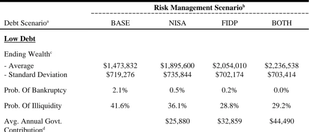
Table 3: Simulation Results for the Hog Farm
Risk Management Scenariob
Debt Scenarioa
BASE NISA FIDP BOTH
Low Debt Ending Wealthc - Average $1,473,832 $1,895,600 $2,054,010 $2,236,538 - Standard Deviation $719,276 $735,844 $702,174 $703,414 Prob. Of Bankruptcy 2.1% 0.5% 0.2% 0.0% Prob. Of Illiquidity 41.6% 36.1% 28.8% 29.2%
Avg. Annual Govt. Contributiond $25,880 $32,859 $44,490 Medium Debt Ending Wealthc - Average $754,381 $1,138,758 $1,300,495 $1,480,533 - Standard Deviation $639,858 $713,644 $694,648 $700,775 Prob. Of Bankruptcy 19.8% 8.3% 4.7% 2.3% Prob. Of Illiquidity 56.3% 50.2% 43.3% 42.6%
Avg. Annual Govt. Contributiond
$25,920 $33,305 $44,971
a
The two debt scenarios are based on initial debt levels, with low representing D/A=0.25 and high representing D/A=0.50.
b The various risk management scenarios are as defined in the main body of the paper. c Statistics for ending wealth are based on all 5000 iterations, with bankruptcy being
represented by zero ending wealth.
d
Government contributions for NISA include matching contributions and interest rate bonus. For FIDP, government contributions are the payments made to producers.
0 10000 20000 30000 40000 50000 60000 70000 80000 1 2 3 4 5 6 7 8 9 10 Year
Net Cash Flow ($)
FIDP
BASE NISA
INSURE
0 20000 40000 60000 80000 100000 120000 140000 1 2 3 4 5 6 7 8 9 10 Year Net Income ($) FIDP BASE NISA INSURE