M
ACHINE
L
EARNING
A
PPROACHES
TO
IMAGE
D
ECONVOLUTION
Dissertation
der Mathematisch-Naturwissenschaftlichen Fakultät
der Eberhard Karls Universität Tübingen
zur Erlangung des Grades eines
Doktors der Naturwissenschaften
(Dr. rer. nat.)
vorgelegt von
Christian Johannes Schuler
aus Nürnberg
Gedruckt mit Genehmigung der Mathematisch-Naturwissenschaftlichen
Fakultät der Eberhard Karls Universität Tübingen.
Tag der mündlichen Qualifikation:
30. 9. 2015
Dekan:
Prof. Dr. Wolfgang Rosenstiel
1. Berichterstatter:
Prof. Dr. Hendrik Lensch
2. Berichterstatter:
Prof. Dr. Bernhard Schölkopf
Summary
Image blur is a fundamental problem in both photography and scientific imaging. Even the most well-engineered optics are imperfect, and finite exposure times cause motion blur. To reconstruct the original sharp image, the field ofimage deconvolutiontries to recover recorded
photographs algorithmically. When the blur is known, this problem is callednon-blind
decon-volution. When the blur is unknown and has to be inferred from the observed image, it is called
blinddeconvolution. The key to reconstructing information lost due to blur and noise is to use
prior knowledge. To this end, this thesis develops approaches inspired by machine learning that include more available information and advance the current state of the art for both non-blind and blind image deconvolution.
Optical aberrations of a lens are encoded in an initial calibration step as a spatially-varying point spread function. With prior information about the distribution of gradients in natural images, the original image is reconstructed in a maximum a posteriori (MAP) estimation, with results comparing favorably to previous methods. By including the camera’s color filter array in the forward model, the estimation procedure can perform demosaicing and deconvolution jointly and thereby surpass the quality of the results yielded by a separate demosaicing step.
The applicability of removing optical aberrations is broadened further by estimating the point spread function from the image itself. We extend an existing MAP-based blind deconvolution approach to the first algorithm that is able to remove spatially-varying lens blurblindly,
inclu-ding chromatic aberrations. The properties of lenses restrict the class of possible point spread functions and reduce the space of parameters to be inferred, enabling results on par with the best non-blind approaches for the lenses tested in our experiments.
To capture more information about the distribution of natural images and capitalize on the abundance of training data, neural networks prove to be a useful tool. As other successful non-blind deconvolution methods, a regularized inversion of the blur is performed in the Fourier domain as an initial step. Next, a large neural network learns the mapping from the preprocessed image back to the uncorrupted original. The trained network surpasses results of state-of-the-art algorithms on both artificial and real-world examples.
For the first time, a learning approach also succeeds in blind image deconvolution. A deep neural network “unrolls” the estimation procedure of existing methods for this task. After training end-to-end on artificially generated example images, the network achieves performance competitive with state-of-the-art methods in the generic case, and even goes beyond when trained for a specific image category.
Zusammenfassung
Unscharfe Bilder sind ein häufiges Problem, sowohl in der Fotografie als auch in der wissen-schaftlichen Bildgebung. Auch die leistungsfähigsten optischen Systeme sind nicht perfekt, und endliche Belichtungszeiten verursachen Bewegungsunschärfe.Dekonvolutionhat das Ziel das
ursprünglich scharfe Bild aus der Aufnahme mit Hilfe vonalgorithmischenVerfahren
wiederher-zustellen. Kennt man die exakte Form der Unschärfe, so wird dieses Rekonstruktions-Problem alsnicht-blindeDekonvolution bezeichnet. Wenn die Unschärfe aus dem Bild selbst inferiert
werden muss, so spricht man vonblinder Dekonvolution. Der Schlüssel zum Wiederherstellen
von verlorengegangener Bildinformation liegt im Verwenden von verfügbarem Vorwissen über Bilder und die Entstehung der Unschärfe. Hierzu entwickelt diese Arbeit verschiedene Ansätze um dieses Vorwissen besser verwenden zu können, basierend auf Methoden des maschinellen Lernens, und verbessert damit den Stand der Technik, sowohl für nicht-blinde als auch für blinde Dekonvolution.
Optische Abbildungsfehler lassen sich in einem einmal ausgeführten Kalibrierungsschritt ver-messen und als eine ortsabhängige Punktverteilungsfunktion des einfallenden Lichtes beschrei-ben. Mit dem Vorwissen über die Verteilung von Gradienten in Bildern kann das ursprüngliche Bild durch eine Maximum-a-posteriori (MAP) Schätzung wiederhergestellt werden, wobei die resultierenden Ergebnisse vergleichbare Methoden übertreffen. Wenn man des Weiteren im Vorwärtsmodell die Farbfilter des Sensors berücksichtigt, so kann das Schätzverfahren Demo-saicking und Dekonvolution simultan ausführen, in einer Qualität die den Ergebnissen durch Demosaicking in einem separaten Schritt überlegen ist.
Die Korrektur von Linsenfehlern wird breiter anwendbar indem man die Punktverteilungs-funktion vom Bild selbst inferiert. Wir erweitern einen existierenden MAP-basierenden Ansatz für blinde Dekonvolution zum ersten Algorithmus, der in der Lage ist auch ortsabhängige opti-sche Unschärfenblindzu entfernen, einschließlich chromatischer Aberration. Die spezifischen
Eigenschaften von Kamera-Objektiven schränken den Raum der zu schätzenden Punktvertei-lungsfunktionen weit genug ein, so dass für die in unseren Experimenten untersuchten Objektive die erreichte Bildrekonstruktion ähnlich erfolgreich ist wie bei nicht-blinden Verfahren.
Es zeigt sich, dass neuronale Netze von im Überfluss vorhandenen Bilddatenbanken profi-tieren können um mehr über die Bildern zugrundeliegende Wahrscheinlichkeitsverteilung zu lernen. Ähnlich wie in anderen erfolgreichen nicht-blinden Dekonvolutions-Ansätzen wird die Unschärfe zuerst durch eine regularisierte Inversion im Fourier-Raum vermindert. Danach ist es einem neuronalen Netz mit großer Kapazität möglich zu lernen, wie aus einem derart
vorver-Zusammenfassung
arbeiteten Bild das fehlerfreie Original geschätzt werden kann. Das trainierte Netz produziert anderen Methoden überlegene Ergebnisse, sowohl auf künstlich generierten Beispielen als auch auf tatsächlichen unscharfen Fotos.
Zum ersten Mal ist ein lernendes Verfahren auch hinsichtlich der blinden Bild-Dekonvolution erfolgreich. Ein tiefes neuronales Netz modelliert die Herangehensweise von bisherigen Schätz-verfahren und wird auf künstlich generierten Beispielen trainiert die Unschärfe vorherzusagen. Nach Abschluss des Trainings ist es in der Lage, mit anderen aktuellen Methoden vergleichbare Ergebnisse zu erzielen, und geht über deren Ergebnisse hinaus, wenn man speziell für eine bestimmten Subtyp von Bildern trainiert.
Papers Included in this Thesis
Papers included in this thesis:
[Sch+11] C. J. Schuler, M. Hirsch, S. Harmeling, and B. Schölkopf. “Non-stationary correction of optical aberrations”. In: IEEE Int. Conf. Computer Vision. 2011. doi: 10.1109/iccv. 2011.6126301
[Sch+12] C. J. Schuler, M. Hirsch, S. Harmeling, and B. Schölkopf. “Blind Correction of Optical Aberrations”. In: Computer Vision – ECCV 2012. Lecture Notes in Computer Science.
Springer, 2012, pp. 187–200. doi:10.1007/978-3-642-33712-3_14
[Sch+13b] C. J. Schuler, H. C. Burger, S. Harmeling, and B. Schölkopf. “A Machine Learning Ap-proach for Non-blind Image Deconvolution”. In:IEEE Conf. Computer Vision and Pattern Recognition. 2013, pp. 1067–1074. doi: 10.1109/cvpr.2013.142
[Sch+14] C. J. Schuler, M. Hirsch, S. Harmeling, and B. Schölkopf. “Learning to Deblur”. In:ArXiv e-prints(2014). arXiv:1406.7444 [cs.CV]. Submitted to a journal.
Papers related to, but not included in this thesis:
[Hir+11] M. Hirsch, C. J. Schuler, S. Harmeling, and B. Schölkopf. “Fast removal of non-uniform camera shake”. In:IEEE Int. Conf. Computer Vision. 2011, pp. 463–470. doi:10.1109/ iccv.2011.6126276
[BSH12c] H. C. Burger, C. J. Schuler, and S. Harmeling. “Image denoising: Can plain Neural Net-works compete with BM3D?”. In: IEEE Conf. Computer Vision and Pattern Recognition.
2012, pp. 2392–2399. doi:10.1109/cvpr.2012.6247952
[BSH12a] H. C. Burger, C. J. Schuler, and S. Harmeling. “Image denoising with multi-layer percep-trons, part 1: comparison with existing algorithms and with bounds”. In: ArXiv e-prints
(2012). arXiv:1211.1544 [cs.CV]
[BSH12b] H. C. Burger, C. J. Schuler, and S. Harmeling. “Image denoising with multi-layer percep-trons, part 2: training trade-offs and analysis of their mechanisms”. In: ArXiv e-prints
(2012). arXiv:1211.1552 [cs.CV]
I would like to thank my co-authors for their permission to base chapters of my thesis on joint publications.
Contents
Introduction 1
1. Fundamentals 5
1.1. Mathematical problem description . . . 6
1.1.1. Stationary convolutions . . . 6
1.1.2. Spatially-varying blur . . . 8
1.2. Non-blind deconvolution methods . . . 10
1.2.1. Wiener deconvolution . . . 11
1.2.2. Tikhonov regularization . . . 11
1.2.3. Recent deconvolution methods . . . 12
1.3. Blind deconvolution methods . . . 13
1.3.1. MAP approaches . . . 13
1.3.2. Marginalization approaches . . . 15
1.4. Neural networks . . . 16
1.4.1. Training . . . 17
1.4.2. Toy example . . . 18
2. Non-Blind Correction of Optical Aberrations 21 2.1. Introduction . . . 21
2.2. Related work . . . 23
2.3. Aberrations as a non-stationary convolution . . . 24
2.4. Forward model including mosaicing . . . 25
2.5. Estimating the non-stationary convolution . . . 26
2.6. Recovering the corrected, full-color image . . . 27
2.7. Results . . . 28 2.7.1. Simulated images . . . 28 2.7.2. Real images . . . 30 2.8. Conclusion . . . 34 2.8.1. Limitations . . . 35 2.8.2. Future work . . . 35
Contents
3. Blind Correction of Optical Aberrations 37
3.1. Introduction . . . 37
3.2. Related work . . . 38
3.3. An efficient filter flow basis for optical aberrations . . . 39
3.4. An orthonormal efficient filter flow basis . . . 40
3.5. Blind deconvolution with chromatic shock filtering . . . 42
3.6. Implementation and running times . . . 45
3.7. Results . . . 45
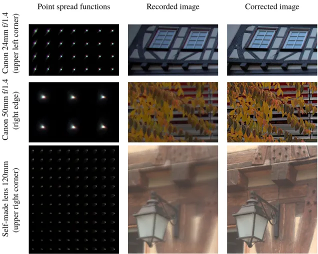
3.7.1. Self-built lens with a single lens element . . . 46
3.7.2. Canon 24mm f/1.4 . . . 46
3.7.3. Kee et al.’s image . . . 46
3.7.4. Historical images . . . 50
3.8. Conclusion . . . 50
3.8.1. Limitations . . . 51
3.8.2. Future work . . . 51
4. Learning Non-Blind Deconvolution 53 4.1. Introduction . . . 53
4.2. Related work . . . 54
4.3. Method . . . 55
4.3.1. Direct deconvolution . . . 55
4.3.2. Artifact removal by multilayer perceptrons . . . 57
4.4. Results . . . 59
4.4.1. Choice of parameter values . . . 59
4.4.2. Comparison to other methods . . . 59
4.4.3. Noise dependence . . . 63
4.4.4. Qualitative results on a real photograph . . . 63
4.5. Understanding . . . 65
4.6. Convolutional training . . . 69
4.6.1. Differences to patch-wise approach . . . 69
4.6.2. Understanding the learned filters . . . 71
4.7. Conclusion . . . 72
5. Learning Blind Deconvolution 75 5.1. Introduction . . . 75
5.2. Related work . . . 76
5.3. Blind deconvolution as a layered network . . . 77
5.3.1. Architecture layout . . . 78
5.3.2. Iterations as stacked networks . . . 81
5.3.3. Training . . . 84
5.4. Implementation . . . 85
5.5. Experiments . . . 85
5.5.1. Image content specific training . . . 85
5.5.2. Noise specific training . . . 87
Contents
5.5.3. Spatially-varying blur . . . 88
5.5.4. Comparisons . . . 90
5.6. Discussion . . . 91
5.6.1. Learned filters . . . 91
5.6.2. Dependence on the size of the observed image . . . 95
5.6.3. Limitations . . . 95
5.7. Conclusion . . . 97
Conclusion and Outlook 99
A. Mathematical Details 103
B. Neural Network Toolbox 107
Acronyms 111
Nomenclature 113
Bibliography 115
Contributions 123
List of Figures
1.1. Illustration of camera shake. . . 6
1.2. Example of an image corrupted by a stationary convolution. . . 7
1.3. Illustration of lens aberrations. . . 8
1.4. Effect of a blur on the power spectrum. . . 10
1.5. Distribution of gradients in natural images. . . 11
1.6. Blind deconvolution procedure for MAP approaches. . . 14
1.7. Intermediate image representations for kernel estimation. . . 15
1.8. Illustration ofp(x,k|y) on a toy example . . . 16
1.9. Classification with a neural network. . . 19
2.1. Self-made photographic lens with one glass element only, mounted on a remote controlled platform. . . 22
2.2. Image taken through self-made lens without and with lens correction. . . 22
2.3. Examples of optical aberrations. . . 24
2.4. Overview of non-blind correction of optical aberrations. . . 26
2.5. Comparison of joint approach vs. sequential demosaicing and deconvolution procedures. . . 29
2.6. Point spread function used for simulations on the Kodak image data set. . . . 31
2.7. Comparison between original and corrected image and the respective PSF. . . 32
2.8. Comparison with DXO for images taken with a Canon EF 50mm f/1.4 lens. . 32
2.9. Interpolation of a mosaiced PSF at the example of a green PSF from the Canon 50mm f/1.4 lens. . . 33
2.10. Comparison with the newer method from [Hei+13] . . . 33
2.11. Comparison of deconvolution with optimization and direct method. . . 34
3.1. Optical aberration as a forward model. . . 39
3.2. Three example groups of patches, each forming a ring. . . 41
3.3. Shifts to generate basis elements for the middle group of Fig. 3.2. . . 41
3.4. SVD spectrum of a typical basis matrixBwith cut-off. . . 41
3.5. Chromatic shock filter removes color fringing. . . 42
3.6. Overview of blind correction of optical aberrations. . . 43
List of Figures
3.8. Comparison between blind approach and two non-blind approaches of Kee et
al. [Kee+11] and DXO. . . 48
3.9. PSF comparison with non-blind approach, self-built lens. . . 49
3.10. Comparison with non-blind approach, Canon 24mm f1/4 lens. . . 49
3.11. Comparison on historical image from 1940. . . 50
4.1. Illustration of the effect of the regularized blur inversion. . . 56
4.2. Overview of learning non-blind deconvolution. . . 57
4.3. Comparison of performance over competitors. . . 60
4.4. Training curves for different MLPs. . . 61
4.5. Comparison of performance for Poisson noise. . . 62
4.6. Images from the best 5% results of scenario (d) as compared to IDD-BM3D. . 64
4.7. Images from the worst 5% results of scenario (d) as compared to IDD-BM3D. 64 4.8. Behavior of the MLP at different noise levels. . . 65
4.9. Removal of defocus blur in a photograph. . . 66
4.10. Feature detectors of an MLP trained to remove a square blur, with preprocessing. 68 4.11. Feature detectors of an MLP trained to remove a square blur, no preprocessing. 68 4.12. Input patterns found via activation maximization vs. feature generators, with preprocessing . . . 68
4.13. Input patterns found via activation maximization vs. feature generators, without preprocessing . . . 68
4.14. Feature detectors of a convolutional NN trained to remove a square blur. . . . 70
4.15. Effect of two filters of a convolutional NN trained to remove a square blur. . . 70
5.1. Architecture of our proposed blind deblurring network. . . 79
5.2. Intermediary outputs of a single-stage NN. . . 80
5.3. Training curves depending on number of stages. . . 82
5.4. Training curves depending on architecture of a single stage. . . 82
5.5. Training curves depending on number of learned gradient-like images. . . 83
5.6. Influence of the learning parameters. . . 83
5.7. Examples of blurs sampled from a Gaussian process. . . 84
5.8. Typical example images ofvalleyandblackboard categories from ImageNet used for content specific training. . . 86
5.9. Comparison of deblurring results for NNs that have been trained with image ex-amples from the entire ImageNet dataset (contentagnostic) and from particular subsets (contentspecific). . . 86
5.10. Comparison of deblurring results for NNs that have been trained with different amounts of noise added to the sample images during training. . . 87
5.11. Comparison onButcher Shopexample of state-of-the-art deblurring methods for removing non-uniform blur together with our estimated PSF. . . 88
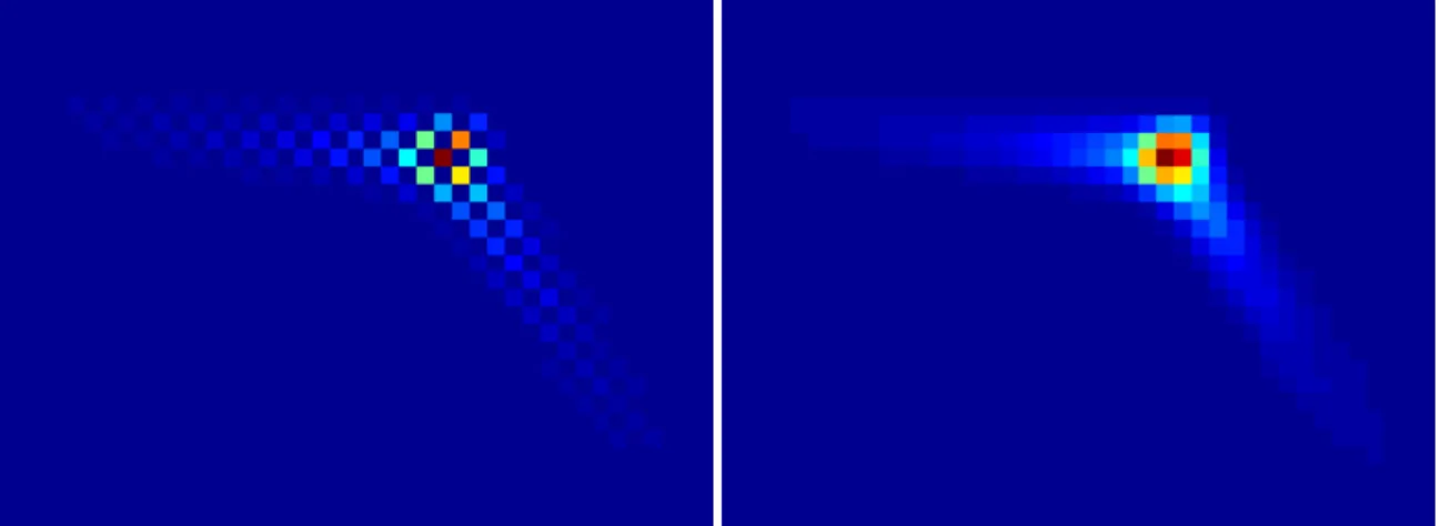
5.12. Visualisation of kernel estimation in the case of spatially-varying blur for the Butcher Shopexample. . . 89
5.13. Results on the benchmark dataset of Levin et al. and the extended benchmark of Sun et al. . . 90
List of Figures
5.14. Comparison on real-world example images taken from the literature with
spa-tially invariant blur. . . 92
5.15. Comparison on real-world example images taken from the literature with spatially-varying blur. . . 93
5.16. Learned filters of the convolution layer for each of the three iterations within a single scale of a trained NN. . . 94
5.17. Comparison of learned filters. . . 94
5.18. Visualization of the effect of the first stage of a network with two predicted output images on toy example with disks blurred with Gaussians of varying size and motion blurred Lena image. . . 95
5.19. Results for kernel estimation for different sizes of the observed image. . . 96
5.20. Dependence of the estimated kernel on the size of the observed image. . . 96
5.21. Failure case of our approach. . . 97
Introduction
Blur is a fundamental problem of physical imaging. Camera optics are never perfect, and typically spread the light emanating from a single point in the scene over several pixels in the sensor plane. It is not always possible to prevent the camera or objects in the scene from moving during image capture, which is especially problematic for long exposure times. In both examples, the result is a blurred image. Blur poses a problem both for everyday photography and scientific imaging, e.g., microscopy or astronomy across all spectral regions from radio waves to gamma rays.
One remedy is to improve the imaging device: using optics with less aberrations, or increas-ing the sensor’s sensitivity to allow smaller exposure times. However, this increases production costs and usually is a trade-off between several target variables. For example, it is easier to minimize aberrations for lenses with small apertures, but small apertures collect less light and increase exposure time. Some limits are even fundamental and independent of current technology (cf. Abbe diffraction limit [BW99]).
Another solution is to recover the original signalcomputationally. This approach belongs to
the class of inverse problems and is called deconvolution. When the blurring process is known a priori (e.g., a fixed optical system that has been measured precisely) the problem is called non-blinddeconvolution. Even though the blur is known, the reconstruction is challenging, because
high frequencies of the signal lose intensity for most blurs, often going towards zero. The noise however, which is an issue without blur in itself, is unaffected in strength and, consequently, can drown the signal. To recover the lost information, prior knowledge has to be incorporated, e.g., in the form of the distribution of the expected image content or the noise.
The reconstruction becomes even more challenging when the blur is not known beforehand. For example, in the case of camera shake, although it is possible to measure the movement of the camera, it is usually impractical. The problem of inferring both the uncorrupted image and the blur is known asblinddeconvolution. Even without noise, the problem is underdetermined since
many combinations of blur and reconstructed image could explain the observation. Again, prior knowledge has to be taken into account for the blind case, in addition to knowledge about the image also about the specifics of the convolution, e.g., camera shake stemming from physically plausible translations and rotations of the camera.
Deconvolution stands as a mature field with many successful applications. Since the 1950s, deconvolution has been used in seismology to infer the Earth’s structure from recorded seis-mograms [Rob54]. The launch of the Hubble space telescope in 1990 motivated the use of
Introduction
deconvolution methods in the field of astronomy, after the telescope’s primary mirror was found to be flawed [Wal90]. Measurements done in the twelve year period until it was repaired necessitated the use of computational corrections. In the field of computational photography, cameras are even designed such that the recorded image has to be post-processed in software, optimizing the full imaging pipeline for a desired property of the final photograph. For example, a coded aperture captures depth information of the scene by adding a depth-dependent blur [Lev+07].
Blur and noise corrupt the information contained within an image. The key idea of recon-structing a signal suffering from loss of information is to use available prior knowledge. Ideally, the prior information contains the full probability distribution of the unknown quantities. Prac-tically, the distribution of all images is computationally intractable, and with respect to its dimensionality only sparsely sampled by even the largest collection of images. Machine Learn-ingprovides tools and methodologies to approximate the distribution explicitly or implicitly,
and thus obtain a prediction for the desired unknown quantity. This could be the most likely solution or the solution otherwise optimal in some sense, e.g., minimizing the expected square error. Using this approach, it is possible to counter the errors introduced by inferior hardware, or for high-quality devices push the boundaries of what is possible.
While image deconvolution is a long-standing problem, and numerous methods exist for both the blind and non-blind case, the work presented in this thesis was able to improve on the state of the art in both cases. Later chapters will demonstrate that we are successful both with maximum a posteriori (MAP) based approaches and with using neural networks to learn to automatically solve the problem of deconvolution.
The outline of this thesis is as follows: after introducing the necessary fundamentals in Chapter 1, we treat the problem ofnon-blind correction of optical aberrations in Chapter 2.
As explained above, optical aberrations cause an unwanted reduction of image quality. A calibration step encodes the spatially-varying aberrations of the optical system. The original image is then reconstructed by solving a MAP problem using a prior on the distribution of gradients in natural images. The results compare favorably to existing approaches for correcting optical aberrations. Additionally, the reconstruction procedure can include demosaicing, and it turns out that treating demosaicing and deconvolution jointly is superior to performing both tasks separately.
Next, the approach in Chapter 3 dispenses with the calibration step and performs blind correction of optical aberrations. Instead of measuring the lens error for every combination of
lens, camera, and setting of the lens, the aberration can be inferred directly from the image. This is the first time blur induced by optical aberrations is correctedblindly. The proposed approach
modifies an existing blind deconvolution method based on MAP and includes domain-specific information to reduce the number of unknown parameters. The class of spatially-varying blurs to be inferred is restricted to a basis of physically plausible lens blurs. Furthermore, blur that is different across multiple color channels can be estimated.
Chapter 4 returns to the basic deconvolution problem with known spatially invariant blur and pushes the state of the art bylearning non-blind deconvolution. An initial preprocessing step
reduces the blur by performing a regularized inversion in Fourier space, a step which is also common in previously existing deconvolution methods. A large neural network is trained on artificially generated training examples to learn the mapping from the preprocessed image back
Introduction
to the uncorrupted original. The trained network achieves state-of-the-art deconvolution results, however, it is specific to a single blur kernel. It is straightforward to include other steps from the imaging pipeline in the reconstruction process, for example demosaicing, as demonstrated on a real-world example.
After the success of a learning method in the non-blind case, the next logical step is to use neural networks forlearning blind deconvolution, which is presented in Chapter 5. Inspired
by existing hand-crafted blind deconvolution methods, a deep neural network “unrolls” the blur estimation by using both conventional layers and layers specific to the problem. The neural network toolbox designed for this procedure is available as open-source software and is described in Appendix B. The proposed method is applicable to both spatially invariant and spatially-varying blurs. After training, the algorithm shows competitive performance on generic blurry images and is superior when trained on specific image categories, where the learning approach can play to its strengths.
CHAPTER
1
Fundamentals
Photography is the process of collecting light which has been emitted or reflected by objects in a scene. As is well-known from physics, light is electro-magnetic radiation that is described by Maxwell’s equations.
The electric and magnetic field strengths present in photography are small enough such that the polarization response of media (the density of induced electric and magnetic dipole moments) can be assumed to be linear. This ignores effects of nonlinear optics, for example the frequency doubling used in green laser pointers to create green light from an infrared laser diode. However, it enables us to model our optical system as alinear system, which means the
superposition principle holds for all electric and magnetic fields. Assuming incoherent light, i.e., electromagnetic waves with random phase differences, this also holds true for the light intensities as measured by the camera.
Ideally, in imaging, light from a single point in the scene should be mapped to a single position on the sensor, excluding cases where for artistic purposes the opposite may be desired. Because of imperfections of the optical system, or movement of the camera during exposure, this is often not the case. Therefore, because of the stated linearity of light, we model the general image formation process as
y =Kx+n. (1.1)
wherexis the vector of the intensities of pixels in the image we would measure in the absence of any errors (a.k.a. ground truth), either for a single color or for an averaged grayscale value. For simplicity, we represent two-dimensional images (or three-dimensional if we consider color) reshaped as vectors. Also, this is a discrete approximation to the continuous signal of the scene. The recorded imageyis obtained after transformation by the matrixK and addition of the measurement noisen, which could optionally also be dependent on the values of the true signalx.
In this work, we will address corruptionsK that can be described as a convolutionlocally,
convo-1. Fundamentals
Figure 1.1.:Left: Image of a grid of light points with stationary motion blur (artificially
created). Middle: Photo of the same grid with spatially-varying motion blur
(non-artifical). Right: Grid of light points for illustration of camera shake
(rear view).
lutions. The task is to recoverxfrom a given observationy. IfKis known, we call the problem
non-blind deconvolution, otherwiseblind deconvolution.
In the following, we introduce the fundamentals necessary for removing blur from images. First, in Section 1.1, we state the mathematical properties of blur in photos. Next, we introduce methods to reconstructxwhen the aberration isknown(Section 1.2) and when it isunknown
(Section 1.3). Lastly, in Section 1.4, we explain the machine learning tools we use to go beyond the established image reconstruction methods.
1.1. Mathematical problem description
To correct for aberrations in images, it is important to be able to describe these aberrations mathematically. In the context of this work, we always work in the domain of discrete pixels in an image (e.g., taken by the sensor of a digital camera), which is an approximation to the continuous domain of the electromagnetic waves which produced this signal.
1.1.1. Stationary convolutions
If the blur is independent of the position within the image, it can be described by a stationary convolution. An example would be a pure translation of the camera parallel to a scene that lies within a single plane, as illustrated in Fig. 1.1 on the left. Mathematically, a convolution is defined as y[n]= (k ∗x)[n]= ∞ X m=−∞ k[m]x[n−m]= ∞ X m=−∞ k[n−m]x[m] (1.2) with functions y,k and x, defined on the set of integersZ, where y[n] denotes the value of y atn. For simplicity, we only show the math for a one-dimensional convolution. Intuitively, ifk is only non-zero near 0, then y[n] is a weighted average of the values ofx nearn, weighted by k. Figure 1.2 shows examples of convolutions in two dimensions, applied to an image.
1.1. Mathematical problem description
Sharp image Convolved with Gaussian blur Convolved with motion blur
Figure 1.2.:Example of an image corrupted by a stationary convolution.
When working on finite domains, there are two noteworthy cases of performing the convolu-tion:
Valid: The finite input vectorxof sizenx is blurred by a kernelkof size nk, resulting in an
outputywith sizenx−nk +1. This is the typical setting in photography, which is physically valid. A pixel on the sensor may receive light from an object outside of the field of view because
of a blur with non-zero extent. Denoting the i-th element of a vectorvasvi, we define y=k ∗ validx where yn= nk X m=1 kmxn+nk−m. (1.3)
Circular: The discrete input signalxis assumed to be periodic with periodnx, this means
y=k ∗ circx where yn = nk X m=1 kmx((n−m)modnx)+1, (1.4)
or creating a circulant matrixK from the entries ofk,
y= Kx. (1.5)
If we perfom the computation as described in this equation, it requiresO(nxnk)
multiplica-tions and addimultiplica-tions, which can be expensive especially for two-dimensional convolumultiplica-tions. We note that the discrete Fourier matrix F diagonalizes a circulant matrixC = FHDiag(Fc)F, where “Diag” creates a diagonal matrix from a vector, cis the first column of C, and FH is the Hermitian transpose of F. Equation (1.5) can be rewritten as the discrete version of the convolution theorem,
y=k∗x= FH(FkFx), (1.6)
since Diag(a)b= aband assuming thatkis zero-padded to the length ofx. The symbol denotes the Hadamard product.
1. Fundamentals
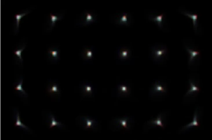
Figure 1.3.:Left: Spatially-varying point spread function (PSF) of a self-built 120 mm
lens. The measurement was performed as described in Section 2.5. Right:
Photo taken with this lens.
Using fast Fourier transforms (FFTs), the discrete Fourier matrix can be multiplied with a vector of length n in timeO(nlogn), which means that the FFT applied to the convolution
theorem enables us to calculateyin timeO(nxlognx). For large blurs the dependence lognx
of this approach versusnk of Eq. (1.4) results in lower computation times. Additionally, as we
will see in Section 1.2, the Fourier representation is especially advantageous when trying to
invert convolutions, i.e., reconstructing the original sharp image.
Revisiting the different convolution types, and introducing an operatorCy which appropri-ately crops a vector by the size of the kernel minus 1 in every dimension, and furthermore an operatorCTk which pads to the size ofx, we obtain:
Valid:
y=Cy (k∗x) =CyFHFCkTkFx. (1.7)
Circular:
y= k∗x= FH FCkTkFx. (1.8)
Note that the transpose of a cropping matrixCis a zero-padding matrixCT.
1.1.2. Spatially-varying blur
Looking at the middle part of Fig. 1.1, a photo of a point grid corrupted by camera-shake, we see that the assumption of stationarity does not always hold for camera shake. This is clear if we consider a rotation of the camera along the axis perpendicular to the image plane: a point in the upper right corner of the image will be shifted in the opposite direction of a point in the lower right corner. However, two points in spatial proximity within the scene will be transformed similarly, this means then the blur variessmoothlyalso across the image plane.
A further example, lens aberrations, exhibits similar behavior, see Fig. 1.3. Again, the corruption islocallya convolution, but varies smoothly across the image plane. In Section 2.3
1.1. Mathematical problem description
we explain the aberrations that cause the incoming light rays to deviate from a single focal point.
We have seen that, in the case of linear optics, Eq. (1.1) is sufficient to describe the image formation process. However, the computational complexity in the general case isO(n2), which
is infeasible for a large number of pixelsnin the ground truth image. Noting that corruptions like camera shake or lens aberrations are still convolutions locally, but vary smoothly, it is
possible to approximate them with the efficient filter flow (EFF) framework [Hir+10]. Its basic idea is to cover the image with overlapping patches, to each of which a blur kernel is assigned.
In this framework, the forward operation is modeled as y=
R X
r=1
k(r)∗ w(r) x, (1.9)
wherexdenotes the ideal image andyis the image degraded by optical aberrations. Herexand yare discretely sampled images, i.e.,xandyare finite-sized vectors whose entries correspond to pixel intensities,w(r) are weighting vectors that mask out all of the imagexexcept for a local patch by Hadamard multiplication. Ther-th patch is convolved appropriately with a local blur kernelk(r) in two dimensions. All blurred patches are summed up to form the degraded image. The more patches are considered (Ris the total number of patches), the better the approximation to the true non-uniform PSF [Hir12]. Note that the patches defined by the weighting vectors w(r)usually overlap to yieldsmoothlyvarying blurs. The weights are chosen such that they sum
up to one for each pixel, i.e.,PR r=1w(
r) = 1, where1denotes a vector of ones. This means that, depending on the weighting vectors, every pixel can have a different blur, a linear combination of the given blur kernels in its neighborhood. Hirsch et al. [Hir+10] show that this forward model can be computed efficiently by making use of the short-time Fourier transform, writing it either in terms ofxork: y= Kx =Cy R X r=1 CrTFHDiagFCkTk(r)FCrDiag w(r) x, (1.10) y= Xk =Cy R X r=1 CrTFHDiag FCrDiag w(r)xFCkTSrk. (1.11)
Adopting the notation of [Hir+10], the matricesCk andCr are appropriately chosen cropping
matrices, and Sr selects k(r) from the kernel stack k. The most expensive operation in this
formulation is the FFT (O(nlogn)), whereas the other operations, including cropping and
zero-padding, are possible to perform in linear time.
From the operator notations in Eqs. (1.10) and (1.11) it is directly clear how to obtain the transpose operatorsKTandXT. These are required for gradient calculations, e.g. when solving deconvolution as an optimization problem. For example, the gradient of the log-likelihood functionE(x) = kKx−yk2, appearing in the next section, would be
∂E ∂x =2K
1. Fundamentals
x k∗x k∗x+n
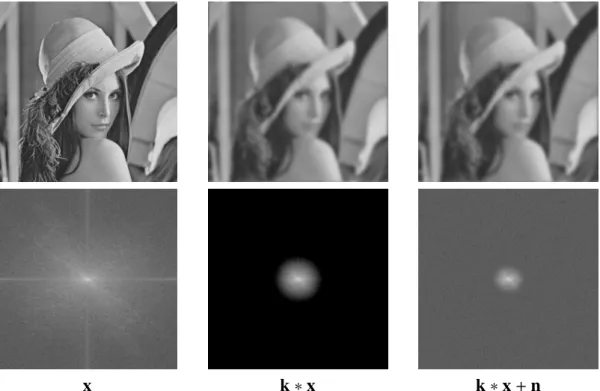
Figure 1.4.:Effect of a blur on the power spectrum. Top row is the image in real space, bottom row the power spectrum on a logarithmic scale. Left:Original image. Center: Blurred with a Gaussian blur. Right: Blurred and with 1% Gaussian
noise. Note how the blur and the noise corrupt high frequencies.
For some cases of spatially-varying blur, alternative representations could be used. For exam-ple for camera shake, the blurry image could be described by a superposition of homographies of the true scene [Why+10]. For lens aberrations, the first few Zernike polynomials approxi-mate the phase of the incoming light well, which is nonlinearly related to the blur throughout the sensor plane [BW99].
1.2. Non-blind deconvolution methods
It is often possible to obtain knowledge about the blur of an image a priori. For example, the aberrations of a lens are fixed, and even motion blur could be measured with accelerometers and gyroscopes [Jos+10].
Given the blur, trying to invert convolution is still an underdetermined problem: we see the effect of a convolution in Fig. 1.4, where the blur lowers the high frequencies. After adding a small amount of noise, the signal-to-noise ratio (SNR) becomes close to 0 in a large part of the spectrum. This is why prior knowledge has to be included to reconstruct the original image from the remaining signal.
1.2. Non-blind deconvolution methods
−0.8 −0.6 −0.4 −0.2 0 0.2 0.4 0.6 0.8
Gradient value
log probability Empirical
Gaussian (α=2) Laplacian (α=1)
Hyper−Laplacian (α=0.63)
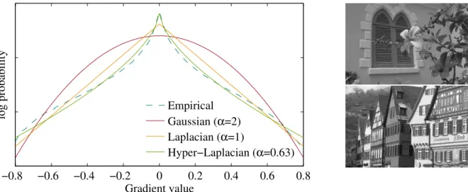
Figure 1.5.:Left: Distribution of horizontal and vertical gradients in natural images
(grayscale). The empirical distribution generated from the Kodak image data set1and fits of three analytic distributions p(x) ∝ exp(−c|x|α) are shown. Right: Two examples from the Kodak image data set.
1.2.1. Wiener deconvolution
In the simplest case, both the signal and the noise, which are additive, are assumed to be
stationary linear stochastic processes, i.e., they have shift-invariant linear joint probability
distribution. This also means that the processes’ spectral properties are sufficient to describe their properties. It can then be shown that the minimum mean square error (MMSE) estimator ˜
xof the original signal is [GW02] ˜
x= FH Fk Fy
|Fk|2+Pn/Px
, (1.13)
assuming circular convolution and thatkis appropriately zero-padded to the size ofx. Here the division, the absolute value and the conjugation (indicated by the bar above a symbol) are point-wise operations. Additionally, we introduced the frequency dependent power spectral density of the noisePnand the signalPx, i.e., the Fourier transform of their respective auto-correlations.
Since this is the MMSE estimator, given our assumptions, there cannot be a better estimator in the square error sense. Comparing Eq. (1.13) with Eq. (1.8), we see thatFk/(|Fk|2+Pn/Px)
acts as a convolution filter on the blurry observationy. This filter is also known as the Wiener filter.
1.2.2. Tikhonov regularization
Contrary to the previous assumptions, images are typicallynot generated by a linear stationary
process, which means that the Wiener deconvolution of Eq. (1.13) can only be an approximation. 1http://r0k.us/graphics/kodak/
1. Fundamentals
Bayes’ rule tells us that the posterior probability density function (PDF) p(x|y)= p(y|x)p(x)
p(y) (1.14)
ofxgiven an observationyis proportional to the likelihoodp(y|x)and the priorp(x),
normal-ized by p(y). From Fig. 1.5 we see that a Gaussian distribution is a rough approximation to
the distribution of gradients in natural images (while a hyper-Laplacian would be better suited, it is also less tractable [KF09]). This provides a prior p(x) ∝ exp−(kGxk2)/(2σ2Gx) with
standard deviationσGx and the gradient matrixG. Assuming Gaussian noise, the likelihood
is p(y|x) ∝ exp−(kk∗x−yk2)/(2σ2n) with standard deviation σn. Then the PDF of x
conditioned onyis p(x|y) ∝exp −kk∗x−yk 2 2σ2 n ! ·exp* , −kGxk 2 2σ2 Gx + -. (1.15)
In the case of a Gaussian distribution the mean and the maximum (a.k.a. mode) are at the same point, the MMSE estimator consequently is the MAP solution. Since the logarithm is a strictly increasing function that does not affect the position of extrema, we can instead determine the minimum of the negative logarithm of the posterior,
ky−k∗xk2+ σ 2 n σ2 Gx kGxk2, (1.16)
Because only L2 norms appear in this objective, in the case of circular convolution there exists a closed-form solution [CL09] x= FH Fk Fy |Fk|2+P i σ2 n σ2 G x |Fgi|2 , (1.17)
assuming that kGxk2can be expressed as the sumP
ikgi∗xk2of convolutions with gradient
filtersgizero-padded to the size ofx. Note that this result is a special case of Eq. (1.13), where Pn= σn21andPx =Piσ2Gx/|Fgi|2.
Unfortunately, the operatorCy that would be necessary for valid convolutions is not diagonal in Fourier space, which breaks the fast inversion by Fourier division. However, this is the convolution type appearing in photography applications. To make it applicable, the blurry image y is tapered in the area of the edges such that there is a smooth transition between opposite edges, e.g., by multiplying the border regions with a window function smoothly going from 1 to 0. [KF09]
1.2.3. Recent deconvolution methods
The methods mentioned above use an explicit image prior (e.g., the Wiener filter incorporates the power spectra of signal and noise) to reconstruct the original signal, and many other methods with more sophisticated explicit image priors are also available. A different class of methods instead tries to first apply the simple deconvolution from Eq. (1.17) and, in a second step, remove the artifacts created from this imperfect reconstruction. We will discuss these two classes of algorithms and their relation to our proposed method in more detail in Section 4.2.
1.3. Blind deconvolution methods
1.3. Blind deconvolution methods
Lenses have many different settings, including aperture, zoom and focus, and inertia sensors for motion blur add additional hardware constraints, making it difficult to measure the exact lens or motion blur. Thus, it is advantageous to infer both the true imagexand the blur kernel from the recorded image, a problem known asblind deconvolution.
In this case, the problem becomes underdetermined even without noise, because many com-binations of blur kernel and reconstructed image could explain the observation. From a prob-abilistic perspective, every pair of kernelk and true image x is associated with a posterior probability
p(x,k|y) = p(y|x,k)p(x)p(k)
p(y) ∝ p(y|x,k)p(x)p(k), (1.18)
analogous to Eq. (1.14). When solving blind deconvolution, we are interested in an estimated solution ˜xand ˜k optimal under a certain loss, i.e., the solution that minimizes the expected errorR
E(x˜,k˜,x,k)p(x,k|y)dxdk with thex- andk-space volume elementsdx anddk, and a given lossE(x˜,k˜,x,k).
For a 0–1 loss, which means that the cost is 0 for the estimated solution equal to the ground truth, and 1 for all wrong solutions, the optimal estimator is the MAP estimator [Mur12] introduced in Section 1.2.2, argmaxx,kp(x,k|y). It is one of the two common approaches for
blind deconvolution. The other approach also considers a 0–1 loss, but only with respect tok, and marginalized overx, i.e., argmaxkp(k|y) = argmaxkR p(x,k|y)dx. In the following we will introduce both approaches.
1.3.1. MAP approaches
The maximum a posteriori approach finds the maximum of Eq. (1.18). As above, this is equiv-alent to the minimum of its negative logarithm. Therefore, we need to minimize
kk∗x−yk2+gx(x)+gk(k) (1.19)
where kk∗x− yk2 is the log-likelihood term under the assumption of Gaussian noise, and
gx(x)andgk(k) are derived fromp(x)andp(k), acting as regularizers in the new objective.
The regularizer gx(x)penalizes blurry images, for example by using a sparse prior on the
gradients [SJA08], which prefers having a single large gradient instead of a smooth transition with many small gradients. While Shan et al. [SJA08] fit to the distribution of gradients of natural images, Xu et al. [XZJ13] are more successful with a sparsity-promoting L0 prior, suggesting that it is more important to be discriminative between sharp and blurry images than to use a generative distribution for sharp images. Similarly, the normalized sparsity measure from [KTF11] is an improper prior since the integral of all prior values is not finite.
Another class of methods only uses implicit regularization for the image, without explicitly defining a regularization termgx(x). For example, this can be achieved by nonlinear filtering
of the image such that edges are emphasized and artifacts are suppressed. Cho and Lee [CL09] apply a shock-filter — the inversion of a diffusion process — and a bilateral filter to achieve this, as can be seen in Figs. 1.7 and 3.5. Another method [XJ10] defines a heuristic procedure to
1. Fundamentals
Current estimate
Next estimate
Feature extraction Kernel estimation Image estimation
Figure 1.6.:Blind deconvolution procedure for MAP approaches. PSF and image estimates are refined by repeating the three stepsfeature extraction,kernel estimation
andimage estimation. The feature extraction shown here creates two images
in gradient space. The kernel and image estimation are often performed by division in Fourier space, hence the division symbol÷.
select gradients that are believed be most informative to estimate the blur kernel. Our proposed method in Chapter 5 also falls into the category of implicit regularization, butlearnsthe optimal
regularization operation.
Having chosen a regularization procedure, MAP approaches iterate between the following three steps, also shown in Fig. 1.6:
Feature extraction: The feature extraction creates image representations that are useful
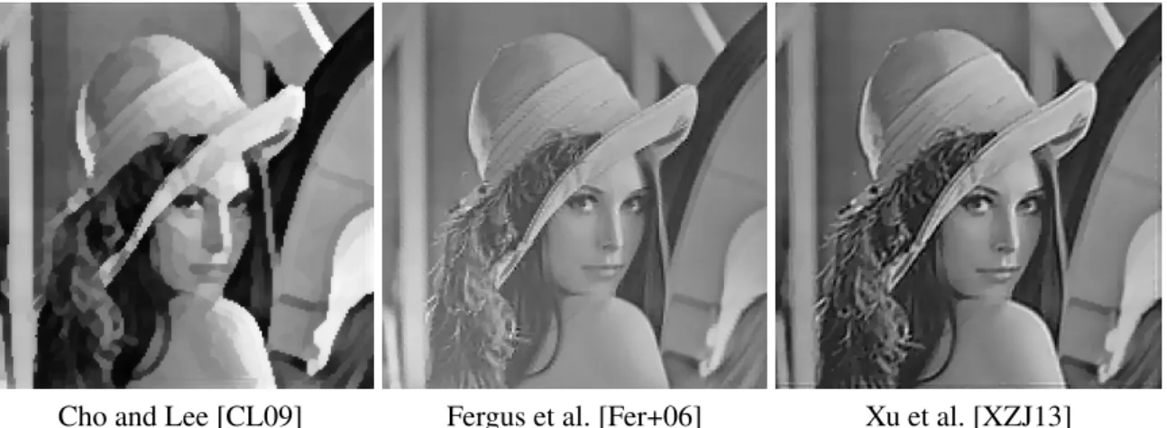
for kernel estimation, using one of the approaches mentioned above. This intermediate feature image is sometimes also called unnatural image representation [XZJ13]. Compared to the sharp image, it is dominated by step-edges and contains less details. The feature extraction is often only performed in gradient space. Figure 1.7 shows a comparison of these intermediate representations, including a direct regularization method [CL09], a marginalization approach [Fer+06] explained below, and a method with implicit regularization [XZJ13] (the latter two reconstructed from gradients).
Kernel estimation: The next step takes the extracted features to estimate the convolution
kernel. The prior on the kernel is often an analytically tractable Gaussian prior, withgk(k) ∝ kkk2 [CL09], or a sparsity-inducing L1 prior gk(k) ∝ kkk1 [SJA08]. It is also possible to
combine a prior with a heuristic approach, e.g., support detection of the kernel [XJ10], to detect the regions where the kernel is non-zero. It is recommended to work on images in gradient space, since in this case the optimization problem converges faster [CL09].
1.3. Blind deconvolution methods
Cho and Lee [CL09] Fergus et al. [Fer+06] Xu et al. [XZJ13]
Figure 1.7.:Intermediate image representations for kernel estimation. These images are intermediate results of blind deconvolution methods analogous to Fig. 1 in [XZJ13]. Fergus’ result has been reconstructed from gradients.
Image estimation: Lastly, the sharp image is estimated using the current kernel estimate,
which will be the starting point for the next feature extraction step.
The three steps are repeated several times on different image scales, starting on a coarse scale with a downsampled version of the blurry image. On the coarser scale the blur is also smaller and easier to infer. After upsampling, the previous solution gives a better initialization for the next scale.
An important consideration of blind deconvolution is to make itfast, i.e., it should ideally
not take more than a few seconds to deblur a standard-sized photo. Usually this requires to solve Eq. (1.19) in a few steps, see Eq. (1.17), instead of performing many iterations with an optimizer. While Eq. (1.17) works only for some regularization terms, e.g., gx(x) ∝ kxk2,
procedures for non-L2 terms exist [KF09; XZJ13].
1.3.2. Marginalization approaches
A toy example for Eq. (1.18) is shown in Fig. 1.8 on the right. While, in this case, the distribution is still simple with both the kernel and image being one-dimensional and only Gaussian priors, in practice local minima pose problems. Additionally, depending on the prior, the trivial solution where the blur is a delta peak can become the global optimum [WZ13], even though regularization schemes as mentioned above can alleviate the problem.
Levin et al. [Lev+09] proposed to instead marginalize overxto obtainp(k|y)= R p(x,k|y)dx and find thekthat maximizes
max
k p(k|y) ≡mink −2 logp(y|k)p(k). (1.20)
Afterwards xcan be obtained by non-blind deconvolution. In the toy example, the marginal is plotted on the left. The advantage of this approach is the reduced dimensionality of the optimization problem. However, marginalizing overxis difficult and can only be done approx-imately, e.g., with variational Bayes (VB) [Lev+11]. As noted by Wipf and Zhang [WZ13],
1. Fundamentals x • max p(x,k|y) • max p(x|y) 0.5 1 1.5 2 2.5 3 3.5 4 0 0.5 1 1.5 2 k p(k|y) p(x,k|y)
Figure 1.8.:Illustration of a toy example withp(x,k|y) ∝ exp −(k2·x−1)2 ·0.12 − x2 2·22 − k2 2·0.52 , and its marginals. The mode of the full distribution is different from the mode of its marginalp(k|y).
the assumptions behind VB are actually not ideal for blind deblurring (e.g., factorization of the distribution). The reported superiority over MAP [Lev+11] seems to be mainly due to avoiding local minima, and the priors should be such that they discriminate well between blurry and sharp images, rather than being generative for sharp images. For a more in-depth review, see [WZ13].
1.4. Neural networks
Another approach does not employ an explicit image priorp(x)butlearnsan estimator from
samples of the ground truthxand the corresponding observationydrawn fromp(x)andp(y|x),
respectively. To draw samples fromp(x), a large collection of photos can be used. We obtain
samples from p(y|x)by applying the corruption process artificially. A learning algorithm can
then obtain information about the intractable distribution p(x)of images implicitly. Artificial
neural networks (NNs) have demonstrated to be successful for this task in the context of image processing [BSH12c], and we will also employ them in this thesis.
While the origins of NNs go back to the 1940s [MP43], they are currently seeing a resurge in popularity, thanks to advances in neural network architectures and faster hardware. NNs are broadly applicable to many different learning tasks and come in many different variants. In the context of this work, NNs meanfeed-forwardneural networks applied tosupervisedlearning
tasks. For a broader picture of NNs, we refer the interested reader to [Sch14].
In our setting, training a NN on a data set is a special case of nonlinear regression, where the function to be learned is a concatenation of elementary functions
f(i) = fn . . . f2 f1(i,p1),p2. . . ,pn. (1.21)
1.4. Neural networks
In the context of neural networks, the building blocks fi(i,pi) of vector-valued functions with
inputiand parameterspiare calledlayers. Given a loss functionE(f(i),t), e.g. a square loss kf(i)−tk2with known input and target pairs iandt, parameterspi can be learned such that
they minimize the expected loss. An architecture often used is the multilayer perceptron (MLP), where the concatenated functions alternate between linear transformations and nonlinearities, e.g.,
f(i) =b3+W3tanh(b2+W2tanh(b1+W1i)), (1.22)
where fi(i,pi) =tanh(bi+Wii)with weight matrixWi and bias vectorbi is commonly called
a hidden layer.
Recently, it has been shown that even this simple architecture can achieve state-of-the-art results for denoising [BSH12c] or digit recognition [Cir+10]. The key difference to older architectures is the use ofdeeparchitectures, meaning four or more of the mentioned layers.
This is also the architecture we use for our non-blind deconvolution algorithm in Chapter 4. For other challenging computer vision problems like object recognition, the NN is a more general layered computation consisting of convolutional layers, pooling layers, normalization layers, or rectifying linear units and other layer types [Le+12]. The learning method for blind deconvolution proposed in Chapter 5 works in the same spirit.
1.4.1. Training
Commonly, NNs are trained withback-propagation[Wer74]. Given a training example with
input and expected output, we can calculate the gradientgiof the loss with respect to a certain
parameter vectorpiby applying the chain-rule: gi= ∂E ∂pi = ∂E ∂fn(i) ∂fn(i) ∂fn−1(i) ∂fn−1(i) ∂fn−2(i) . . .∂fi(i) ∂pi . (1.23)
We see that the derivative of a layeri includes all derivatives∂fj(i)/∂fj−1(i) of subsequent layers. The intermediate results can be reused from layer to layer, which means the derivative isback-propagated. Next, every layer is updated by changing the parameters as
pi(t+1) =pi(t)+∆pi(t). (1.24) One possible approach to adapt the network’s parameters in order to minimize the cost on a training set is the stochastic gradient descent (SGD) algorithm [Bot91]. Every update is the scaled gradient
∆pi(t) = −ηgi(t) (1.25)
with learning rateη. Note that “stochastic” means that the update is calculated on a random selection of training examples. The convergence rate can be improved by adapting the learning rate layer-wise (e.g., dividing by a factor depending on the input dimension of each layer [LeC+98b]).
The momentum update rule [RHW86] includes not only the current gradient, but the past gradients with exponentially decaying importance, ∆pi(t) = Ptτ−=10ρτgi(t−τ). This smoothens random variations orthogonal to the dominant gradient direction.
1. Fundamentals
Fast convergence rates and less tuning for different architectures are achieved by the ADA-GRAD [DHS11] method. It normalizes the update with the root mean square (RMS) of all previous gradients, effectively setting a different learning rate for every parameter:
∆pi(t) =−η/ v t t X τ=1 (gi(τ))2·gi(t), (1.26) where all operations are performed element-wise. The diverging RMS of the past gradients causes the updates to go to zero over time, which may be desired to reduce overfitting on limited training data.
When near infinite training data is available, for example when sampling from a generative model, this behavior may be undesired. The ADADELTA [Zei12] method proposes to include past gradients in the calculation of the RMS with decaying importance,
∆pi(t) = −ηRMS[∆pi] (t−1) RMS[gi](t) gi(t) with RMS[g](t) = q E[g2](t)+ and E[g2](t) = ρE[g2](t−1)+(1− ρ)g(t)2. (1.27) Additionally, it adds a speed-up term in the numerator, which becomes large when the previous updates are large.
The methods mentioned here are often performed on several training examples simultane-ously, called mini-batches, where multiple gradients are combined to a single, more meaningful gradient. This can be advantageous because some operations in the neural network need less instructions if performed over multiple inputs, as compared to multiple executions on a single in-put. A good example is a single matrix-matrix multiplication instead of multiple matrix-vector multiplications.
To successfully train NNs, there are many other important design choices, for example num-ber of hidden units, and “tricks”, like the initialization of the parameters pi, data normalization
or layer-wise hyper-parameter settings discussed in [Ben12].
1.4.2. Toy example
Neural networks have proven to be successful for classification and regression tasks. How do they achieve this? To give some insights, we trained2a small MLP to solve a two dimensional classification task with two classes which are not linearly separable (see Fig. 1.9 on the left). The network has two input dimensions, one hidden layer with two dimensions, and two output classes, allowing us to plot the intermediary and final outputs in their full dimensionality. While commonly one hidden layer in an MLP means both a nonlinearity and an affine transformation, we here view the affine transformation as separate layers.
The network maps an inputito an outputowhereok is the probability ofibelonging to a
class k of K total classes. When providing labelstk for the training data (1 if its true class
is k, otherwise 0), we can train the network on the cross-entropy loss −PKk tkln(ok) using
2We employed ConvNetJS (http://github.com/karpathy/convnetjs) for both training and visualization.
1.4. Neural networks
Input-Layer Linear-Layer Tanh-Layer Linear-Layer Softmax-Layer
Hidden layers
Figure 1.9.:Classification with a neural network. This toy example shows an MLP with two input dimensions, “one” hidden layer with two neurons (the linear layers are commonly discounted in the number of hidden layers) and two output classes. See Section 1.4.2 for details.
the training procedure of our choice, here SGD. While the network may converge to different parameter configurations, one successful outcome after training is a network that performs the following operations on the input:
1. Linear layer:The first hidden layer applies an affine transformationo1=b1+W1i. We see from Fig. 1.9 that the input plane is rotated such that the two directions which could separate the classes are aligned to the coordinate system of the feature space.
2. Tanh layer:Next, the data is nonlinearly transformed aso2= tanh(o1), “straightening out”
the region between the different classes, and making the two classes linearly separable. 3. Linear layer: A second affine transformationo3= b3+W3iprojects out the dimension
along the line separating the two classes in the nonlinear feature space, since the network decided this dimension is not relevant for the classification decision. Also, the output of the linear layer is rotated relative to its input to be suitable for the subsequent softmax layer.
4. Softmax layer: The final output layer converts its input into the normalized probability
of a certain point belonging to a particular class, i.e.,o= exp(o3)/PKk=1exp(o3,k). The
colored areas in Fig. 1.9 depict in red or green where the probability for class 1 or 2 is larger than 0.5, respectively. At the red end of the line the NN is certain that the corresponding point in the input layer belongs to class 1, at the green end that it belongs to class 2.
We see that the MLP transformed the nonlinearly separable input to a nonlinear feature space, where it islinearlyseparable, allowing a classification decision.
CHAPTER
2
Non-Blind Correction of Optical Aberrations
Taking a sharp photo at several megapixel resolution traditionally relies on high grade lenses. In this chapter, we present an approach to alleviate image degradations caused by imperfect optics. We rely on a calibration step to encode the optical aberrations in a space-variant point spread function and obtain a corrected image by non-stationary deconvolution. By including the Bayer array in our image formation model, we can perform demosaicing as part of the deconvolution.
The material of this chapter is based on the following publication:
[Sch+11] C. J. Schuler, M. Hirsch, S. Harmeling, and B. Schölkopf. “Non-stationary correc-tion of optical aberracorrec-tions”. In: IEEE Int. Conf. Computer Vision. 2011. doi:
10. 1109/ iccv. 2011. 6126301
2.1. Introduction
In an ideal optical system as described theoretically by paraxial optics, all light rays emitted by a point source converge to a single point in the focal plane, forming a clear and sharp image. Departures of an optical system from this behavior are called aberrations, causing unwanted blurring of the image.
Manufacturers of photographic lenses attempt to minimize optical aberrations by combining several lenses. The design and complexity of a compound lens depends on various factors, e.g., aperture size, focal length, and constraints on distortions. Optical aberrations are inevitable and the design of a lens is always a trade-off between various parameters, including price. To correct these errors in software is still an unresolved problem.
Rather than proposing new designs for complicated compound lenses, we show that almost all optical aberrations can be corrected by digital image processing. For this, we note that optical aberrations of a linear optical system are fully described by their PSF. We will show
2. Non-Blind Correction of Optical Aberrations
Figure 2.1.:Self-made photographic lens with one glass element only, mounted on a re-mote controlled platform to take photos in different angles.
Figure 2.2.:Image taken through self-made lens without and with lens correction.
how various optical aberrations encountered in real photographic lenses can be represented and approximated as PSFs in non-stationary convolutions, as mentioned in Section 1.1.2. For a given lens/camera combination, the parameters of the non-stationary convolution are estimated via an automated calibration procedure that measures the PSF at a grid covering the image. We also include demosaicing into our image reconstruction, because it fits naturally into our forward model. Our results surpass the previous state of the art.
Main contributions: We show how to reconstruct a full-color image, i.e., all three color
channels at full resolution, given a raw image that is corrupted by various monochromatic and chromatic aberrations, and Bayer filtered by a color filter array (CFA) of our off-the-shelf camera. This image reconstruction is even possible for heavily degraded images, taken with a self-constructed lens consisting of asingle lens elementattached to a standard camera, see
Fig. 2.1.
2.2. Related work
2.2. Related work
There exist many different methods solely for demosaicing, for reviews see [Ram+02; Gun+05; AL08; LGZ08]. However, none of them model and exploit the spatially-varying aberration of the lens to facilitate demosaicing as our method does. Most closely related is a MAP approach that treats deconvolution and demosaicing jointly [ST09], but for blur constant across the image and all color channels.
Chromatic aberrations arise because the refractive index of glass, and thus focal length and image scale, is dependent on the wave length. A common approach to correct for lateral chromatic aberrations is a non-rigid registration of the different color channels [BW92; KL05; MW07]. Such methods correspond to restricting our model to delta-peaked PSFs, and generally ignore other optical aberrations. The method of [CKS09] measures chromatic aberration at edges through color differences and compensates locally, however without using a PSF model of the lens. The approach in [JSK08] also relies on the estimation of sharp step edges and can be used in a non-blind fashion. Even though full PSFs are estimated, they are only used to remove chromatic aberrations, where a rough knowledge of the PSF is sufficient. None of these approaches consider demosaicing.
A method that focuses on correcting coma has been proposed in [Gif08], showing how to reduce coma by locally applying blind deconvolution methods to image patches. This method is designed for grayscale images and thus does neither consider chromatic aberration nor de-mosaicing.
Algorithmically related to our work is [FEM06], considering sparsity regularization in the luminance channel, and Tikhonov regularization in the two chromaticity channels. However, [FEM06] combines the image information from several images, while our method works with a single image. Also, [FEM06] combines demosaicing with super-resolution, while we combine it with correction for chromatic aberrations.
The image reconstruction problem we are addressing can also be dealt with using the propri-etary software “DxO Optics Pro” (DXO), which tries to correct for image aberrations. DXO is considered state-of-the-art among professional photographers and presumably uses the same kind of information as our approach (it contains a custom database of lens/camera combina-tions). It has been developed over a number of years and is highly optimized. DXO states that it can correct for “lens softness”, which their website1defines as image blur that varies across the image and between color channels in strength and direction. It is not known to us whether DXO models the blur as space-variant defocus blur of different shapes or with more flexible PSFs as we do; neither do we know whether DXO demosaics and deblurs simultaneously as we do. In the experimental section we show that our results compare favorably with results obtained by DXO.
Using deconvolution to correct for lens aberrations is also discussed in [Kee+11]. This work focuses on removing lens blur across multiple aperture and zoom settings of a given lens. A calibration method similar to [JSK08] is used. While this method can correct aberrations across many different settings of a lens, the blur shape is modelled as a Gaussian. As can be seen in 1https://web.archive.org/web/20110519014422/http://dxo.com/us/photo/dxo_optics_pro/
2. Non-Blind Correction of Optical Aberrations
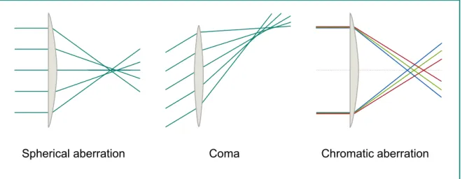
Spherical aberration Coma Chromatic aberration
Figure 2.3.:Examples of optical aberrations: light rays are not focused into a single point. Fig. 2.9 this is not appropriate for strong aberrations considered in this paper. Also, the problem of demosaicing is not treated.
There exist several papers which suggest calibration procedures to measure the lens, e.g. [SA94; Ste02; JSK08]. However, they mainly focus on correcting geometric distortion or do not address monochromatic aberrations.
A closely related method published after the material of this chapter also infers the spatially-varying PSF in a measurement step and removes the blur algorithmically [Hei+13]. It obtains the lens aberration from a calibration pattern and then performs non-blind deconvolution with a cross-channel term designed to minimize color fringing.
2.3. Aberrations as a non-stationary convolution
While the aberrations of an imaging system can be described as a simple matrix operator, we have noted in Chapter 1 that the required matrix-vector multiplication would be computationally expensive. As can be seen in Fig. 2.7 on the left, the aberration can also be represented as PSFs that vary in size, shape, orientation and intensity, depending on the position in the image. Since the PSFs also vary smoothly across the image plane, using EFF (Section 1.1.2) is a valid approximation in this case.
Lenses are affected by a variety of different aberrations. Each of them have in common that light rays are not focused into a single point anymore. In the following, we explain the categories of aberrations that we can include in our model and remove in the reconstruction step:
Monochromatic aberrations. This class of aberrations includesspherical aberration(in
spherical lenses, the focal length is a function of the distance from the axis, see Fig. 2.3 on the left) as well as a number of off-axis aberrations: comaoccurs in an oblique light bundle
when the intersection of the rays is shifted with respect to its axis (Fig. 2.3 in the middle);
field curvatureoccurs when the focal surface is non-planar;astigmatismdenotes the case when
2.4. Forward model including mosaicing
the sagittal and tangential focal surfaces do not coincide (i.e., the system is not rotationally symmetric for off axis light bundles);distortion, which is the only aberration we do not address,
is related to a spatially-varying image scale. All these monochromatic aberrations lead to blur that varies across the image. Any such blur can be expressed in the EFF framework by appropriately choosing the local blur kernelsk(1), ...,k(R) in Eq. (1.9).
Chromatic aberration. The refraction index of most materials including glass is dependent
on the wavelength of the transmitted light. Axially, this results in the focus of a lens being a function of the wavelength (longitudinal chromatic abe