Hajji, W and Tso, FP
Understanding the Performance of Low Power Raspberry Pi Cloud for Big
Data
http://researchonline.ljmu.ac.uk/3778/
Article
LJMU has developed LJMU Research Online for users to access the research output of the University more effectively. Copyright © and Moral Rights for the papers on this site are retained by the individual authors and/or other copyright owners. Users may download and/or print one copy of any article(s) in LJMU Research Online to facilitate their private study or for non-commercial research. You may not engage in further distribution of the material or use it for any profit-making activities or any commercial gain.
The version presented here may differ from the published version or from the version of the record. Please see the repository URL above for details on accessing the published version and note that access may require a subscription.
For more information please contact [email protected]
http://researchonline.ljmu.ac.uk/
Citation
(please note it is advisable to refer to the publisher’s version if you
intend to cite from this work)
Hajji, W and Tso, FP (2016) Understanding the Performance of Low Power
Raspberry Pi Cloud for Big Data. Electronics, 5 (2). ISSN 2079-9292
Article
Understanding the Performance of Low Power
Raspberry Pi Cloud for Big Data
Wajdi Hajji * and Fung Po Tso *
Department of Computer Science, Liverpool John Moores University, Liverpool L3 3AF, UK
*Correspondence: [email protected] (W.H.); [email protected] (F.P.T.); Tel.: +44-7438-981273 (W.H.) Academic Editors: Simon Cox and Steven Johnston
Received: 30 April 2016; Accepted: 31 May 2016; Published: 6 June 2016
Abstract:Nowadays, Internet-of-Things (IoT) devices generate data at high speed and large volume. Often the data require real-time processing to support high system responsiveness which can be supported by localised Cloud and/or Fog computing paradigms. However, there are considerably large deployments of IoT such as sensor networks in remote areas where Internet connectivity is sparse, challenging the localised Cloud and/or Fog computing paradigms. With the advent of the Raspberry Pi, a credit card-sized single board computer, there is a great opportunity to construct low-cost, low-powerportable cloudto support real-time data processing next to IoT deployments. In this paper, we extend our previous work on constructing Raspberry Pi Cloud to study its feasibility for real-time big data analytics under realistic application-level workload in both native and virtualised environments. We have extensively tested the performance of a single node Raspberry Pi 2 Model B withhttperf and a cluster of 12 nodes withApache SparkandHDFS (Hadoop Distributed File System). Our results have demonstrated that our portable cloud is useful for supporting real-time big data analytics. On the other hand, our results have also unveiled that overhead for CPU-bound workload in virtualised environment is surprisingly high, at 67.2%. We have found that, for big data applications, the virtualisation overhead is fractional for small jobs but becomes more significant for large jobs, up to 28.6%.
Keywords: internet of things; Raspberry Pi; Raspberry Pi Cloud; Micro Data Centre; big data; virtualisation; Docker; energy consumption
1. Introduction
Low-cost, low-power embedded devices are ubiquitous, part of the Internet-of-Things (IoT). These devices or things include RFID tags, sensors, actuators, smartphones,etc., which have substantial impact on our everyday-life and behaviour [1]. Today’s IoT devices generate data at remarkable speed which requires near real-time processing [2]. Such need has inspired a new computing paradigm that advocates moving computation to the edge, closer to where data are generated for ensuring low-latency and responsive data analytics [2]. Examples are localised Cloud Computing [3] and Fog Computing [2].
Both localised Cloud and Fog Computing paradigms work only in populous environment embedded with rich and high-speed connectivity. However, in many cases IoT devices are deployed in inaccessible remote areas which have limited or no Internet connectivity to the outside world [4]. Lacking of connectivity effectively prevents these isolated IoT devices from accessing to either localised Cloud or Fog Computing. This calls for a radically new computing paradigm which: (1) is capable of processing data efficiently; (2) has the agility of Cloud Computing; (3) is portable to support on-demand physical mobility; and (4) is low-cost, low-power for sustainable computing in remote areas.
This new computing paradigm has been made possible by the emergence of low-cost, low-power credit card-sized single board computer—the Raspberry Pi [5]. As a result, there has been some Electronics2016,5, 29; doi:10.3390/electronics5020029 www.mdpi.com/journal/electronics
pioneering novel networked systems with the Raspberry Pi. These innovative systems include a high performance computing (HPC) cluster [6] and a scale model cloud data centre [7].
This style of system offers many advantages. The system is easy to provision at small scale and requires minimal outlay. We have extended our original project in [7] and constructed a cloud of 200 networked Raspberry Pi 2 boards for US$ 9,000. Such systems are highly portable, running from a single AC mains socket, and capable of being carried in a luggage.
In this paper, we have carried out an extensive set of experiments with representative real-life workloads in order to understand the performance of such system in big data analytics. In summary, the contribution of this paper is as follows:
• We designed and conducted a set of experiments to test the performance of a single node and
a cluster of 12 Raspberry Pi 2 boards with realistic network and CPU bound workload in both native and virtualised environments.
• We have found that overhead for CPU-bound workload in virtualised environment is significant,
giving up to 67.2% performance impairment.
• We have found that the performance of running big data analytic in virtualised environment
comparable to native counterpart, albeit noticeable but trivial overhead for CPU, memory and energy.
The rest of this paper is organised as follows: Section 3gives an overview of background technologies on Apache Spark and HDFS, the big data analytic tools used for experiments. We present details of our experiment setups in Section4, followed by description and analysis of our experiment results in Section 5. We survey related literature and highlight our contribution in Section 2. And Section6concludes the paper.
2. Related Work
Since its launch in 2012, the Raspberry Pi has quickly become one of the best-selling computers and has stimulated various interesting projects across both industry and academia that fully exploit the low cost low power full feature computer [6–11]. As of 29 February 2016, the total number of units sold worldwide has passed 8 million [12].
Iridis-pi [6] and Glasgow Raspberry Pi Cloud [7] are among the first to use a large collection of Raspberry Pi boards to construct clusters. Despite their similarity in hardware construction, their nature is distinctively different. Iridis-pi is an educational platform that can be used to inspire and enable students to understand and apply high-performance computing and data handling to tackle complex engineering and scientific challenges. On the contrary, the Glasgow Raspberry Pi cloud is an educational and research platform which emphasises development and understanding virtualisation and Cloud Computing technologies. Other similar Raspberry Pi clusters include [8,13,14].
In spite of their popularity, there is surprisingly limited study on the performance of ab individual node and a whole cluster under realistic workload. The author of [15], has run experiments to test container-based technology on a single node Raspberry Pi. They evaluate the virtualisation impact on CPU, Memory I/O, Disk I/O, and Network I/O and conclude that overhead is negligible compared with native execution. However, the experiments focus mainly on the system level benchmarking and do not represent realistic workload. The author of [8], studies energy consumption out of a 300-node cluster but without a more representative workload. The author of [16], has studied the feasibility of Raspberry Pi 2 based cluster built out of seven nodes for big data applications with more realistic workloads using Apache Hadoop framework. The TeraSort is used to evaluate the cluster performance and energy consumption that is reported.
In contrast to [8,15,16], our work concentrates on evaluation of system performance under realistic application layer workload, featuring various workloads inhttperf and Apache Spark. In addition, we study and report the performance with and without virtualisation layer, which offers improved insight into the suitability of virtualisation for a low-power, low-cost computer cluster. Our methodology is
also partly inspired by [17], which evaluated the performance of Spark andMapReducethrough a set of diverse experiments for an x86 cluster.
3. Background 3.1. Spark
Apache Spark (https://spark.apache.org/docs/latest) is a general-purpose cluster computing system. Spark can play the role of traditional ETL (extract, transform, and load) for data processing and feeding data warehouses, and it can also perform other operations such as on-line pattern spotting or interactive analysis.
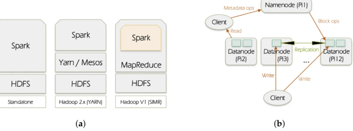
Figure1a illustrates the ways in which Spark can be built and deployed upon Hadoop components. There are: (1) Standalone mode: where Spark interacts with HDFS directly but MapReduce could collaborate with it in the same level to run jobs in cluster; (2) Hadoop Yarn: Spark just runs over Yarn which is a Hadoop distributed container manager; (3) Spark in MapReduce (SIMR): in this case Spark can run Spark jobs in addition to the standalone deployment.
Spark Spark MapReduce Yarn / Mesos HDFS Spark HDFS HDFS
Standalone Hadoop 2.x (YARN) Hadoop V1 (SIMR)
(a) Namenode (Pi1) Client Client Datanode (Pi2) Datanode (Pi3) Datanode (Pi12) Write Replication
...
(b)Figure 1. Spark and HDFS (Hadoop Distributed File System) overview. (a) Spark deployment; (b) HDFS architecture.
Spark generally processes data through the following stages: (1) the input data are distributed on worker nodes; (2) then data are processed by themapperfunctions; (3) following that,shuffling process performs aggregation of similar patterns; and finally (4)reducerscombine them all to get a consolidated output.
In our experiments we have adopted Spark Standalone deployment. Both Spark and HDFS are in cluster mode. In total there are 12 nodes, one Raspberry Pi represents the master and the others represent workers.
3.2. HDFS
HDFS (https://wiki.apache.org/hadoop/HDFS/) is a distributed file system designed to run on commodity hardware. It is designed to handle large datasets. HDFS distributes and replicates data on the cluster members to protect system against failure that could happen due to nodes unavailability.
HDFS follows the master-slave paradigm. A HDFS cluster is composed of a namenode which is the master (Pi1), it manages the file system name-space and regulates clients’ access to files, and it also distributes blocks/data on the datanodes. Datanode can be present in each node of the cluster. It is responsible for serving read and write requests from the file system’s clients, it also manages blocks creation, deletion, and replication according to the instructions coming from the namenode. Figure1b depicts the HDFS architecture.
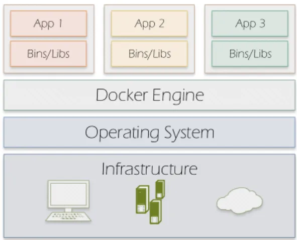
3.3. Docker
Docker (https://www.docker.com/what-docker) allows applications packaging with all their dependencies into software containers. Different from the Virtual Machine design which requires an entire operating system to run the applications on, Docker enables sharing the system kernel between containers by using the resource isolation features available on Linux environment such as cgroups and kernel namespaces. Figure2illustrates Docker’s approach.
Infrastructure
Operating System
Docker Engine
App 1 Bins/Libs App 2 Bins/Libs App 3 Bins/LibsFigure 2.Docker containers.
4. Experiment Setup
We describe in detail our testbed, methodology and performance metrics used to evaluate different combinations of tests in this section.
In an edge cloud we anticipate two distinctive environments—either a native environment for high performance or a virtualised environment for high elasticity. Therefore, we have tested the performance of single nodes and clusters in both environments. In all experiments we either use a single node Raspberry Pi 2 Model B, which has a 900 MHz quad-core ARM Cortex-A7 CPU, 1 G RAM, and a 100 Mbps Ethernet connection, or a cluster of 12 nodes. For their virtualised counterparts, we have configured the node(s) with Docker, a lightweight Linux Container virtualisation, on each Raspberry Pi with Spark and HDFS running atop. We have chosen Spark because it has become one of the most popular big data analytics tools. We selected Docker not only because it is low-overhead OS level virtualisation but also the full virtualisation has not been fully supported by Raspberry Pi 2’s hardware. The operating system (OS) installed on the Raspberry Pis is Raspbian (https://www.raspbian.org/). 4.1. Single Node Experiments
In this set of experiments, we attempt to find the baseline performance with and without virtualisation for a single Raspberry Pi 2 Model B board. The experiments include using a client, which has an Intel i7-3770 3.4 GHz quad-core CPU, 16 GB RAM and 1 Gbp/s Ethernet, sending various workload to server, a Raspberry Pi node, usinghttperf[18]. The client used is remarkably more powerful than the server for ensuring that performance will only be limited by server’s bottleneck. The server runs Apache web server to process web requests from client. The client is instructed to generate a large number of Web (HTTP) requests for pulling web documents of size 1 KB, 4 KB, 10 KB, 50 KB, 70 KB and 100 KB respectively from servers usinghttperf. These workload sizes are chosen because traffic in cloud data centre is comprised of 99% small mice flows and 1% large flows [19]. For each specific workload size, the client starts from sending a very small number of requests per second to the server initially, and gradually increases the number of requests per second by 100 until
the server cannot accommodate any additional requests. This means that the server has reached its full capacity.
4.2. Cluster Experiments
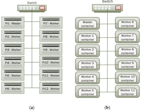
We have conducted all experiments on a low-power compute cluster consist of 12 Raspberry Pi 2 Model B. All Raspberry Pis are interconnected with a 16-Port Gbp/s switch. Alongside with system performance metrics, we are equally interested in energy consumption of the whole cluster when experiment is underway. We used MAGEEC (http://mageec.org/wiki/Workshop) ARM Cortex M4-based STM32F4DISCOVERY board to measure energy consumption of individual Raspberry Pi throughout experiments. This board was designed by the University of Bristol for high frequency measurement of energy usage.
Also on each node, we installed Spark 1.4.0 and Hadoop 2.6.4 for its HDFS. We configured node 1, i.e., Pi 1, as a master for Hadoop and Spark, and others,i.e., Pi 2–12, as workers.
For Spark, each worker was allocating 768 MB RAM and all 4 CPU cores. For HDFS, we set the number of replica to 11 so that data are replicated on each worker node. This set-up was not only considered for high availability but also to avoid high network traffic between nodes as we predict that Raspberry Pi has a hardware limitation on the network interface speed. Figure3a shows the cluster design.
Swi tch
Pi1 - Master Pi7 - Worker
Pi2 - Worker Pi8 - Worker
Pi3 - Worker
Pi4 - Worker
Pi9 - Worker
Pi10 - Worker
Pi5 - Worker Pi11 - Worker
Pi6 - Worker Pi12 - Worker
(a) Switch Worker 1 conta iner Worker 2 conta iner Worker 3 conta iner Worker 4 conta iner Master conta iner Worker 5 conta iner Worker 7 conta iner Worker 8 conta iner Worker 9 conta iner Worker 10 conta iner Worker 6 conta iner Worker 11 conta iner (b)
Figure 3.Cluster Layout. (a) Native set-up; (b) Virtualised set-up.
In the second phase of the experiment, we installed Docker and created a Docker container on each node of the cluster. Docker container hosts both Spark 1.4.0 and Hadoop 2.6.4 with the same setup as in the native environment. So the container is considered as a Virtual Machine running on the Raspberry Pi. We have established a network connection between the 12 containers and have made them able to communicate between each other. Figure3b illustrates this set-up.
In both native and virtualised environments, we have run bothWordcountandSortjobs on our low-power cluster with job sizes varying from 1 GB to 4 GB and to 6 GB, representing small, medium and large job sizes respectively. The large job size was set to 6 GB because we have found that job size greater than this will cause Docker daemon forcibly killed by the OS because the CPU is
significantly overloaded with the process. Also in all experiments we left the system idle for 20 s and the experiments started at the 21-st s.
In all experiments, we have measured and collected the following metrics to examine the performance:
• Execution time: the time taken by each job running different workloads.
• Network throughput: the transmission and reception rates in each node of the cluster. • CPU utilisation: the CPU usage in each cluster node.
• Energy consumption: energy consumed by a Raspberry Pi worker node (chosen randomly).
5. Experiment Results 5.1. Single Node Performance
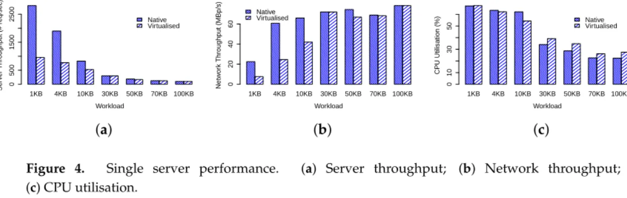
Our test results for single node performance are shown in Figure4. We first examine the results for native environment. Obviously, Figure4a shows that the average number of network requests served by the server decreases from 2809 req/s to 98 req/s for 1 KB and 100 KB workloads respectively. In the meantime, their corresponding network throughput, as shown in Figure4b and CPU utilisation, as shown in Figure4c exhibit monotonically increasing and decreasing patterns respectively, but with flatter tails. The average network throughput for 1 KB and 100 KB workloads are 22.5 Mbp/s and 78.4 Mbp/s respectively, whereas CPU utilisation for 1 KB and 100 KB workloads are 67.2% and 22.3% respectively. These observations demonstrate that small-sized workloads such as 1 KB and large-sized workloads such as 100 KB are CPU and network bounded respectively.
1KB 4KB 10KB 30KB 50KB 70KB 100KB Workload Ser v er Throughput (# req/sec) 0 500 1500 2500 Native Virtualised (a) 1KB 4KB 10KB 30KB 50KB 70KB 100KB Workload Netw or k Throughput (MBp/s) 0 20 40 60 Native Virtualised (b) 1KB 4KB 10KB 30KB 50KB 70KB 100KB Workload CPU Utilisation (%) 0 10 30 50 Native Virtualised (c)
Figure 4. Single server performance. (a) Server throughput; (b) Network throughput; (c) CPU utilisation.
Next we examine the results for virtualised environment. At first glance we can clearly observe that all results for virtualised environment exhibit identical patterns as native environment. However, our performance has pinpointed significant virtualisation overhead, particularly for small workloads. Figure4a shows that server throughput for 1 KB workload is profoundly impaired by 65.9%, dropping from 2, 809 req/s to 957.5 req/s, leading to significant degradation in network throughput (Figure 4b) while the CPU utilisation remains equally high as native counterpart. Similarly the impairment for 4 KB and 10 KB workloads are 59.6% and 36.4% respectively. Nevertheless, the performance for large workloads including 30 KB, 50 KB, 70 KB and 100 KB, in terms of server and network throughput, are on par with their native counterparts. In comparison the CPU utilisation for these workloads are only 12%–23%, representing fractional but significant overhead.
The remarkable overhead observed for the small-sized workloads has inspired us to investigate this issue further. When Docker is installed, a software-based bridged network, by which the Docker daemon connects containers to this network by default, is automatically created. Therefore, when workload is small not only the hardware network interface frequently interrupts CPU for packet delivery but also the software bridge triggers similar amount of interrupts for container under test. On the contrary, when workload is large, fewer hardware and software interruptions arise from both physical and virtual network interface.
5.2. Spark and HDFS in the Native Environment
We first present Spark’s performance in the native environment. Table1shows the total execution time for 1 GB, 4 GB and 6 GB jobs. We observed that job completion time varies with actual job sizes. For instance, forWordCount, it increases slightly from 60.2 s for 1 GB job by 9.3% to 65.8 s for 4 GB job but increases substantially by 82.4% to 109.8 s for 6 GB job. Similar trend is observed inSort, it takes 122.4 s to complete 1 GB job, then 129.7 s and 224.8 s, or 5.96% and 83.7% longer, for 4 GB and 6 GB files respectively. Comparing job completion time betweenWordCountandSort, it is apparent thatSortis more CPU demanding because time taken bySortjob is almost usually double of what is consumed by WordCount. This is because inSort, words need to be counted and then sorted, whereas inWordCount words need only to be counted.
Table 1.Execution times for WordCount and Sort jobs in the Native Environment.
File Size “Native” WordCount “Native” Sort
1 GB 60.2 s 122.4 s
4 GB 65.8 s 129.7 s
6 GB 109.8 s 224.8 s
To explain this non-linear increase in completion time between 4 GB and 6 GB jobs, we have investigated further and found thatSort for 4 GB job requires 32 tasks whilst 6 GB file needs 46. Given that there are 44 cores available in the cluster, there is sufficient computation capacity for accommodating 32 task concurrently. However, in the case when 45 or more tasks are spawn, all available cores are used, as demonstrated in Figure 5c, and the remaining tasks will have to wait for CPU time. Worse still, if they depend on some specific tasks, they will have to wait until their completion although free CPU time will arise when some non-dependent tasks finish early. On the other hand, Spark is memory hungry whilst Raspberry Pi’s RAM is sparse. As evidenced by Figure5c, memory has been fully utilised at most of the time throughout experiments. This implies that there may be constant memory swapping that could further lengthen the completion time. InWordCount, there are 15 tasks for 4 GB file versus 44 for 6 GB file, in the former case there are enough CPU resources to run all tasks whereas in the latter all CPU cores are dedicated to run the job, this can be observed in Figure5c where CPU usage is at 100% over data processing time whilst it is at nearly 80% for 4 GB file in Figure5b. 0 20 40 60 80 100 120 140 160 0 20 40 60 80 100 120 140 % Time (s) CPU-WordCount Mem-WordCount CPU-Sort Mem-Sort (a) 0 20 40 60 80 100 120 140 160 0 20 40 60 80 100 120 140 160 % Time (s) CPU-WordCount Mem-WordCount CPU-Sort Mem-Sort (b) 0 20 40 60 80 100 120 140 160 0 50 100 150 200 250 300 % Time (s) CPU-WordCount Mem-WordCount CPU-Sort Mem-Sort (c)
Figure 5.CPU and memory usage. (a) 1 GB file; (b) 4 GB file; (c) 6 GB file.
Next, we describe the CPU, memory and network usage performance results. InWordCountof 1 GB job, in Figure5a memory consumption increases to about 75% and remains steady till the end of the operation. For CPU utilisation, we can see that it rises from nearly 1% (idle) to nearly 20% (busy)
and remains unchanged all over the computation process. For network throughput, Figure6a shows that there is no significant traffic activity, at the beginning of the job, data are received by workers at the rate of 40 kb/s, and this is the client (namenode) request message for workers to start computing. For files of 4 GB and 6 GB, we noted the same behaviour but the increase in CPU and memory usage is more prominent. For instance, in Figure5b for 4 GB file, memory usage increases gradually from 50% to 100% in about 70 s and CPU goes up from nearly 1% to 30% in thetasks submissionstage and then sharply reaches 80% at the second 40 for thecountstage as indicated in the log files.
0 500 1,000 1,500 2,000 2,500 3,000 3,500 0 20 40 60 80 100 120 140 kb /s Time (s) TX-WordCount RX-WordCount TX-Sort RX-Sort (a) 0 1,000 2,000 3,000 4,000 5,000 6,000 7,000 8,000 9,000 10,000 0 20 40 60 80 100 120 140 160 kb /s Time (s) TX-WordCount RX-WordCount TX-Sort RX-Sort (b) 0 2,000 4,000 6,000 8,000 10,000 12,000 0 50 100 150 200 250 300 kb /s Time (s) TX-WordCount RX-WordCount TX-Sort RX-Sort (c)
Figure 6.Network transmission (TX) and reception (RX) rates. (a) 1 GB file; (b) 4 GB file; (c) 6 GB file.
As reflected by Figure5c the increase is sharper for the 6 GB file where both memory and CPU reach 100%. In the 6 GB file, as explained above, since there are more tasks (46 tasks) than available CPU cores (44 cores), the CPU and memory are exhaustively used for an extended period of time. Moreover, we observe the same two stages as in the 4 GB file.
InSort, CPU and network usage patterns are different from those observed inWordCountjob. For example, in Figure5a for the 1 GB job, CPU usage increases to the same level asWordCountjob for the same file size, and it remains steady throughout the experiment, but at the end of the job CPU decreases dramatically to a very low level and then suddenly reaches a peak. When analysing log files, we have found an explanation for these changes. In the beginning,tasks submissionstage takes a few seconds to complete, this is happening also inWordCount, it explains both CPU and memory increase to 30% and 60% respectively. Afterwards,mapstage starts and consumes most of the time taken by the job, lastly theshufflingprocess causes the peak witnessed by CPU usage.
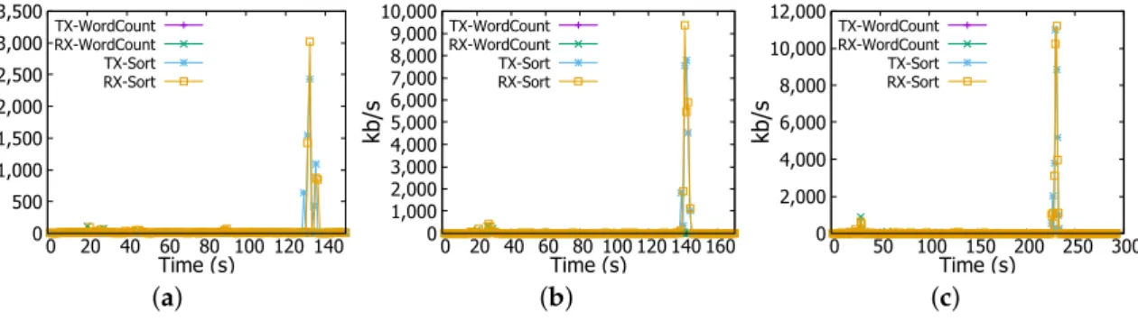
In addition,Sortis accompanied with a peak in the network transmission and reception rates where they reach nearly 3.2 Mbps as shown in Figure6a. Same changes have been witnessed for 4 GB and 6 GB files but with quantitative differences. For instance, as illustrated in Figure6b,c network transmission and reception rates reach at the end of theSortjob 9.6 Mbps and nearly 11.2 Mbps for 4 GB and 6 GB files respectively. CPU and memory usages increase as well to nearly 80% and 100% for 4 GB file and to 100% and 100% for 6 GB file respectively as reflected in Figure5b,c. These changes are explained above by the fact thatSortjob witnesses three phases;task submission,map, andshuffling. In the shuffling stage, a high network activity is noticed at the end ofSortjob (e.g., Figure5a at 130 s, Figure5b at 140 s, and Figure5c at 235 s). Furthermore, outputs coming from workers need to be consolidated to have the final result, this is achieved in thereducestage (combining results of workers) and it causes the high CPU and memory usage.
Regarding the energy consumption, through Figures7a and8a we can obviously observe that actual energy consumption depends on the job sizes. It is slightly higher for 6 GB files than for 1 GB and 4 GB files in bothWordCountandSortjobs. To confirm this observation, we runWordCountand Sorton file of 8 GB, even with some task failures on some Raspberry Pis, we noticed the behaviour more clearly as shown in Figures7b and8b. Therefore, workload affects the energy consumption, the more intensive the workload is, the more important is the energy consumption by the Raspberry Pi device.
3.62e-005 3.64e-005 3.66e-005 3.68e-005 3.70e-005 3.72e-005 0 20 40 60 80 100 120 Jo ul e Time (s) WordCount 6GB WordCount 4GB WordCount 1GB (a) 3.68e-005 3.70e-005 3.72e-005 3.74e-005 3.76e-005 3.78e-005 3.80e-005 3.82e-005 0 20 40 60 80 100 120 Jo ul e Time (s) WordCount 8GB WordCount 4GB WordCount 1GB (b)
Figure 7.Energy measurement in a Raspberry Pi Worker node in WordCount job. (a) WordCount Job (1-4-6 GB files); (b) WordCount Job (1-4-8 GB files).
3.62e-005 3.64e-005 3.66e-005 3.68e-005 3.70e-005 3.72e-005 0 20 40 60 80 100 120 140 160 180 Jo ul e Time (s) Sort 6GB Sort 4GB Sort 1GB (a) 3.68e-005 3.70e-005 3.72e-005 3.74e-005 3.76e-005 3.78e-005 3.80e-005 3.82e-005 0 20 40 60 80 100 120 140 160 Jo ul e Time (s) Sort 8GB Sort 4GB Sort 1GB (b)
Figure 8.Energy measurement in a Raspberry Pi Worker node in Sort job. (a) Sort job (1-4-6 GB files); (b) Sort job (1-4-8 GB files).
5.3. Spark and HDFS in Docker-Based Virtualised Environment
In the second phase of our experiments, we present results from virtualised environment, followed by comparing and contrasting the results with that of native ones.
We first have a look at the job completion time as shown in Table2. At the first glance, we can clearly see that job completion times for 1 GB and 4 GB exhibit fractional difference, smaller than 3%, between native and virtualised platforms for bothWordCountandSort.
Table 2.Execution times for WordCount and Sort jobs in Virtualised Environment.
File Size WordCount in Docker Sort in Docker
1 GB 58.2 s 121.1 s
4 GB 64.7 s 132.2 s
6 GB 116.5 s 236.5 s
However, inWordCountof 6 GB file, execution with Docker clearly takes more time than the case without it, at 109.8 s and 116.5 s respectively, an increase of nearly 6.1%. Similarly,Sorton the 6 GB file takes more time in Docker than in the native environment, an increase from 224.8 s to 236.5 s, representing 5.2% longer completion time.
5.3.1. Virtualisation Impact on CPU and Memory Usage
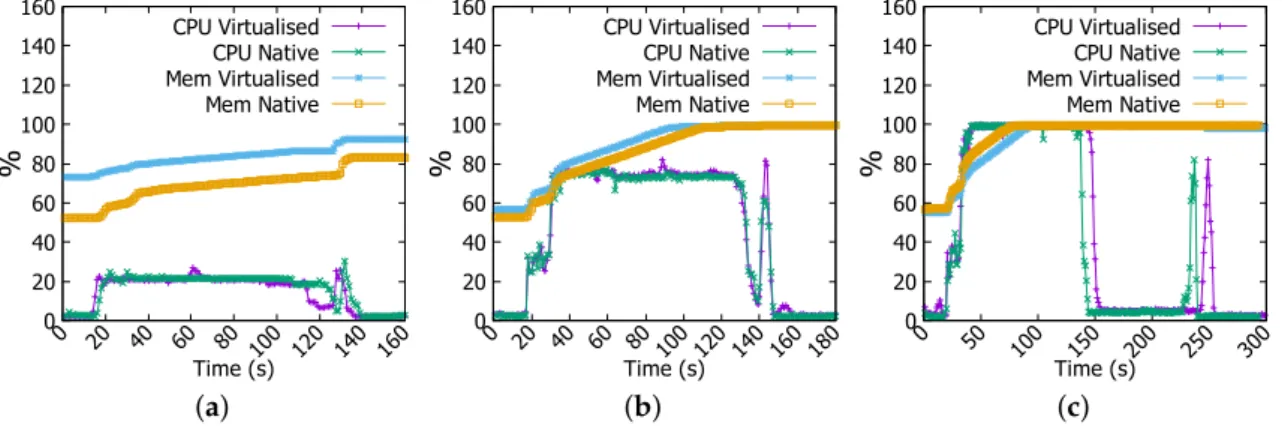
Figure9a shows that CPU usage, in 1 GB fileWordCountjob, has same behaviour in both native and virtualised environments but with a few irregularities where Docker is running (at 20-th and 50-th s). Memory consumption is higher in virtualised platform as Docker daemon requires already memory resources to run its processes. InWordCountof 4 GB file, CPU and memory usages have the same patterns in both environments (Figure 9b). Whereas, inWordCount of 6 GB file, we have noticed remarkable difference in the CPU usage, Figure9c shows that it is more important and extended in the virtualised set-up. 0 20 40 60 80 100 120 140 160 0 20 40 60 80 100 120 % Time (s) CPU Virtualised CPU Native Mem Virtualised Mem Native (a) 0 20 40 60 80 100 120 140 160 0 20 40 60 80 100 120 % Time (s) CPU Virtualised CPU Native Mem Virtualised Mem Native (b) 0 20 40 60 80 100 120 140 160 0 20 40 60 80 100 120 % Time (s) CPU Virtualised CPU Native Mem Virtualised Mem Native (c)
Figure 9.CPU and memory usage in WordCount job. (a) 1 GB file; (b) 4 GB file; (c) 6 GB file.
InSortjob of 1 GB file, the difference only resides in the memory usage. With Docker, memory consumption is higher than is the case in the native environment as unveiled in Figure10a. We have also noticed a few irregularities in CPU usage in virtualised environment. As for the 4 GBSortjob, Figure10b demonstrates nearly identical patterns in both environments. Figure10c demonstrates a more obvious difference in CPU utilisation between two environments in which virtualised platform exhausts CPU resource earlier and for longer periods of time.
0 20 40 60 80 100 120 140 160 0 20 40 60 80 100 120 140 160 % Time (s) CPU Virtualised CPU Native Mem Virtualised Mem Native (a) 0 20 40 60 80 100 120 140 160 0 20 40 60 80 100 120 140 160 180 % Time (s) CPU Virtualised CPU Native Mem Virtualised Mem Native (b) 0 20 40 60 80 100 120 140 160 0 50 100 150 200 250 300 % Time (s) CPU Virtualised CPU Native Mem Virtualised Mem Native (c)
Figure 10.CPU and memory usage in Sort job. (a) 1 GB file; (b) 4 GB file; (c) 6 GB file.
These set of experiments have demonstrated that virtualisation incurs a more prominent overhead when the jobs are more demanding.
5.3.2. Virtualisation Impact on Network Usage
Figure11a shows thatWordCountdoes not produce significant network traffic with two spikes at the rate of 140 kb/s. Similarly, Figure11b shows very small difference in network throughput for 4 GB job inWordCount. However, the network behaviour becomes different for 6 GB job. Network reception
rate becomes more intensive in the native environment than it is in the virtualised counterpart as shown in Figure11b. For example, at 28-th s reception rate in virtualised environment reaches nearly 600 kb/s while in the native environment it is nearly at 900 kb/s.
0 20 40 60 80 100 120 140 0 10 20 30 40 50 60 70 80 kb /s Time (s) TX Virtualised TX Native RX Virtualised RX Native (a) 0 100 200 300 400 500 600 0 10 20 30 40 50 60 70 80 kb /s Time (s) TX Virtualised TX Native RX Virtualised RX Native (b) 0 100 200 300 400 500 600 700 800 900 0 10 20 30 40 50 60 70 80 kb /s Time (s) TX Virtualised TX Native RX Virtualised RX Native (c)
Figure 11.Transmission (TX) and reception (RX) rates in WordCount job. (a) 1 GB file; (b) 4 GB file; (c) 6 GB file.
In Sort job, we have noticed a different network behaviour from the case in WordCount. In Figure12a there is a high network traffic at the end of the experiment, this is a consequence of the shufflingprocess where workers are sharing results for consolidation. Reception and transmission rates are more intensive in the native environment than where Docker is running. In Figure12b we have found identical behaviour in network usage in both environments, however the rate is higher than it is in 1 GB file for the same job; transmission and reception rates reach nearly 9.600 Mbps.
0 500 1,000 1,500 2,000 2,500 3,000 3,500 0 20 40 60 80 100 120 140 kb /s Time (s) TX Virtualised TX Native RX Virtualised RX Native (a) 0 1,000 2,000 3,000 4,000 5,000 6,000 7,000 8,000 9,000 10,000 0 20 40 60 80 100 120 140 160 kb /s Time (s) TX Virtualised TX Native RX Virtualised RX Native (b) 0 2,000 4,000 6,000 8,000 10,000 12,000 0 50 100 150 200 250 300 kb /s Time (s) TX Virtualised TX Native RX Virtualised RX Native (c)
Figure 12.Transmission (TX) and reception (RX) rates in Sort job. (a) 1 GB file; (b) 4 GB file; (c) 6 GB file.
Lastly, we can see from Figure12c that network usage is remarkably more intensive in the native environment. For instance reception and transmission rates reach 11.2 Mbps in the native environment while they are at nearly only 8 Mbps in virtualised one. The difference is about 3.2 Mbps or 28.6%. 5.3.3. Virtualisation Impact on Energy Consumption
In this section, we will investigate how much overhead, if any, virtualisation has in terms of energy consumption.
Figure13a depicts the energy consumed by a Raspberry Pi cluster worker member when it is involved inWordCountjob on 1 GB file, energy levels are very similar. However forWordCounton 4 GB file, energy is more important in the native environment than in virtualised one as shown in Figure13b. However, inWordCountfor 6 GB job, as revealed in Figure13c energy level becomes clearly higher when jobs are running inside Docker containers. It arises from 3.66×10⁻⁵Joule to 3.71×10⁻⁵Joule, so
an increase of 1.3%. ForSortjob, same patterns have been observed for the case of 4 GB and 6 GB jobs as shown in Figure14b,c.
3.61e-005 3.62e-005 3.63e-005 3.64e-005 3.65e-005 3.66e-005 3.67e-005 3.68e-005 3.69e-005 3.70e-005 0 10 20 30 40 50 60 Jo ul e Time (s) Virtualised Native (a) 3.55e-005 3.60e-005 3.65e-005 3.70e-005 3.75e-005 0 10 20 30 40 50 60 Jo ul e Time (s) Virtualised Native (b) 3.65e-005 3.70e-005 3.75e-005 3.80e-005 3.85e-005 0 20 40 60 80 100 120 Jo ul e Time (s) Virtualised Native (c)
Figure 13.Energy measurement in WordCount job. (a) 1 GB file; (b) 4 GB file; (c) 6 GB file.
3.55e-005 3.60e-005 3.65e-005 3.70e-005 3.75e-005 0 20 40 60 80 100 120 Jo ul e Time (s) Virtualised Native (a) 3.55e-005 3.60e-005 3.65e-005 3.70e-005 3.75e-005 0 20 40 60 80 100 120 140 Jo ul e Time (s) Virtualised Native (b) 3.65e-005 3.70e-005 3.75e-005 3.80e-005 3.85e-005 0 20 40 60 80 100 120 140 Jo ul e Time (s) Virtualised Native (c)
Figure 14.Energy measurement in Sort job. (a) 1 GB file; (b) 4 GB file; (c) 6 GB file.
6. Conclusions
In this paper, we have designed and presented a set of extensive experiments on a Raspberry Pi cloud using Apache Spark and HDFS. We have evaluated their performance through CPU and memory usage, Network I/O, and energy consumption. In addition, we have investigated the virtualisation impact introduced by Docker, a container-based solution that relies on resources isolation features available on Linux kernel. Unfortunately, it has not been possible to use Virtual Machines as a virtualisation layer because this technology is not yet supported in the current releases on Raspberry Pi. Our results have shown that the virtualisation effect becomes more clear and distinguishable with high workloads, e.g., when operating on a big amount of data. In a virtualised environment, CPU and memory consumption becomes higher, network throughput decreases, and burstiness occurs less often and less intensively. Furthermore, it has been proven that energy level consumed by the Raspberry Pi arises with the high workload and it is additionally affected by the virtualisation layer where it becomes more important. As a future work, we are interested in attenuating the virtualisation overhead by investigating a novel traffic management scheme that will take into consideration both network latency and throughput metrics. This scheme will mitigate network queues and congestion at the levels of virtual appliances deployed in the virtualised environment. More precisely, it will rely on three keystones; (1) controlling end-hosts packets rate; (2) virtual machines and network functions placement; and (3) fine-grained load-balancing mechanism. We believe this will improve the network and applications performance but it will not have a significant impact on the energy consumption.
References
1. Atzori, L.; Iera, A.; Morabito, G. The internet of things: A survey. Comput. Netw.2010,54, 2787–2805. 2. Bonomi, F.; Milito, R.; Zhu, J.; Addepalli, S. Fog Computing and Its Role in the Internet of Things.
In Proceedings of the 1st Edition of the MCC Workshop on Mobile Cloud Computing, Helsinki, Finland, 13–17 August 2012; pp. 13–16.
3. Choy, S.; Wong, B.; Simon, G.; Rosenberg, C. A hybrid edge-cloud architecture for reducing on-demand gaming latency.Multimed. Syst.2014,20, 503–519.
4. Yoneki, E. RasPiNET: Decentralised Communication and Sensing Platform with Satellite Connectivity. In Proceedings of the 9th ACM MobiCom Workshop on Challenged Networks, CHANTS’14, New York, NY, USA, 7 September 2014; pp. 81–84.
5. Raspberry Pi Foundation. Raspberry Pi 2, 2012. https://www.raspberrypi.org/products/raspberry-pi-2 -model-b/ (accessed on 25 April 2016).
6. Cox, S.J.; Cox, J.T.; Boardman, R.P.; Johnston, S.J.; Scott, M.; O’brien, N.S. Iridis-pi: A low-cost, compact demonstration cluster. Clust. Comput.2014,17, 349–358.
7. Tso, F.P.; White, D.R.; Jouet, S.; Singer, J.; Pezaros, D.P. The Glasgow Raspberry Pi Cloud: A Scale Model for Cloud Computing Infrastructures. In Proceedings of the 2013 IEEE 33rd International Conference on Distributed Computing Systems Workshops (ICDCSW), Philadelphia, PA, USA, 8–11 July 2013; pp. 108–112. 8. Abrahamsson, P.; Helmer, S.; Phaphoom, N.; Nicolodi, L.; Preda, N.; Miori, L.; Angriman, M.; Rikkila, J.; Wang, X.; Hamily, K.; et al. Affordable and Energy-Efficient Cloud Computing Clusters: The Bolzano Raspberry Pi Cloud Cluster Experiment. In Proceedings of the 2013 IEEE 5th International Conference on Cloud Computing Technology and Science (CloudCom), Bristol, UK, 2–5 December 2013; Volume 2, pp. 170–175.
9. Fernandes, S.L.; Bala, J.G. Low Power Affordable and Efficient Face Detection in the Presence of Various Noises and Blurring Effects on a Single-Board Computer. InEmerging ICT for Bridging the Future, Proceedings of the 49th Annual Convention of the Computer Society of India (CSI) Volume 1, Hyderabad, India, 12–14 December 2014; Springer: CH-6330 Cham (ZG), Switzerland, 2015; pp. 119–127.
10. Jain, S.; Vaibhav, A.; Goyal, L. Raspberry Pi Based Interactive Home Automation System Through E-mail. In Proceedings of the 2014 International Conference on Optimization, Reliabilty, and Information Technology (ICROIT), Faridabad, India, 6–8 February 2014; pp. 277–280.
11. Vujovi´c, V.; Maksimovi´c, M. Raspberry Pi as a Wireless Sensor node: Performances and Constraints. In Proceedings of the 2014 37th International Convention on Information and Communication Technology, Electronics and Microelectronics (MIPRO), Opatija, Croatia, 26–30 May 2014; pp. 1013–1018.
12. Raspberry Pi Foundation. Raspberry PI 3 On Sale Now, 2016. https://www.raspberrypi.org/blog/ raspberry-pi-3-on-sale/ (accessed on 25 April 2016).
13. Anwar, A.; Krish, K.R.; Butt, A.R. On the Use of Microservers in Supporting Hadoop Applications. In Proceedings of the 2014 IEEE International Conference on Cluster Computing (CLUSTER), Madrid, Spain, 22–26 September 2014; pp. 66–74.
14. Cloutier, M.F.; Paradis, C.; Weaver, V.M. Design and Analysis of a 32-Bit Embedded High-Performance Cluster Optimized for Energy and Performance. In Proceedings of the 2014 Hardware- Software Co-Design for High Performance Computing (Co-HPC), New Orleans, LA, USA, 17 November 2014; pp. 1–8.
15. Morabito, R. A performance evaluation of container technologies on internet of things devices. 2016, arXiv:1603.02955. arXiv.org e-Print archive. Available online: http://arxiv.org/abs/1603.02955 (accessed on 20 April 2016).
16. Schot, N. Feasibility of Raspberry Pi 2 based Micro Data Centers in Big Data Applications. In Proceedings of the 23th University of Twente Student Conference on IT, Enschede, The Netherlands, 22 June 2015.
17. Shi, J.; Qiu, Y.; Minhas, U.F.; Jiao, L.; Wang, C.; Reinwald, B.; Özcan, F. Clash of the Titans: MapReducevs.
Spark for Large Scale Data Analytics. In Proceedings of the VLDB Endowment, Kohala Coast, HI, USA, September 2015; Volume 8, pp. 2110–2121.
18. Mosberger, D.; Jin, T. Httperf—A tool for measuring web server performance.ACM SIGMETRICS Perform. Eval. Rev.1998,26, 31–37.
19. Greenberg, A.; Hamilton, J.R.; Jain, N.; Kandula, S.; Kim, C.; Lahiri, P.; Maltz, D.A.; Patel, P.; Sengupta, S.
VL2: A Scalable and Flexible Data Center Network. InACM SIGCOMM Computer Communication Review;
ACM: New York, NY, USA, 2009; Volume 39, pp. 51–62. c
2016 by the authors; licensee MDPI, Basel, Switzerland. This article is an open access article distributed under the terms and conditions of the Creative Commons Attribution (CC-BY) license (http://creativecommons.org/licenses/by/4.0/).