Farouk Salem
School of Science
Thesis submitted for examination for the degree of Master of Science in Technology.
Espoo 22 June, 2016
Thesis supervisor:
Assoc. Prof. Keijo Heljanko
Thesis advisor:
Author: Farouk Salem
Title: Comparative Analysis of Big Data Stream Processing Systems
Date: 22 June, 2016 Language: English Number of pages: 12+77 Department of Computer Science
Supervisor: Assoc. Prof. Keijo Heljanko Advisor: D.Sc. (Tech.) Khalid Latif
In recent years, Big Data has become a prominent paradigm in the field of dis-tributed systems. These systems distribute data storage and processing power across a cluster of computers. Such systems need methodologies to store and process Big Data in a distributed manner. There are two models for Big Data processing: batch processing and stream processing. The batch processing model is able to produce accurate results but with large latency. Many systems, such as billing systems, require Big Data to be processed with low latency because of real-time constraints. Therefore, the batch processing model is unable to fulfill the requirements of real-time systems.
The stream processing model tries to address the batch processing limitations by producing results with low latency. Unlike the batch processing model, the stream processing model processes the recent data instead of all the produced data to fulfill the time limitations of real-time systems. The subsequent model divides a stream of records into data windows. Each data window contains a group of records to be processed together. Records can be collected based on the time of arrival, the time of creation, or the user sessions. However, in some systems, processing the recent data depends on the already processed data.
There are many frameworks that try to process Big Data in real time such as Apache Spark, Apache Flink, and Apache Beam. The main purpose of this research is to give a clear and fair comparison among the mentioned frameworks from different perspectives such as the latency, processing guarantees, the accuracy of results, fault tolerance, and the available functionalities of each framework.
Keywords: Big Data, Stream processing frameworks, Real-time analytic, Apache Spark, Apache Flink, Google Cloud Dataflow, Apache Beam, Lambda Architecture
Acknowledgment
I would like to express my sincere gratitude to my thesis supervisor Assoc. Prof. Keijo Heljanko for giving me this research opportunity and providing me continuous motivation, support, and guidance in my research. I also would like to give very special thanks to my instructor D.Sc. (Tech.) Khalid Latif for providing very helpful guidance and directions throughout the process of completing the thesis. I’m glad to thank my fellow researcher Hussnain Ahmed for the thoughtful discussions we had. Last but not the least, I would like to thank my parent and my wife as the main source of strength in my life and special thanks to my child, Youssof for putting me back in the mood everyday.
Thank you all again.
Otaniemi, 22 June, 2016
Abbreviations and Acronyms
ABS Asynchronous Barrier Snapshot API Application Program Interface D-Stream Discretized Stream
DAG Directed Acyclic Graph FCFS First-Come-First-Serve FIFO First-IN-First-OUT GB Giga Byte
HDFS Hadoop Distributed File System NA Not Applicable
MB Mega Byte
RAM Random Access Memory RDD Resilient Distributed Dataset RPC Remote Procedure Call SLA Service-Level Agreement TCP Transmission Control Protocol UDF User-Defined Function
UID User Identifier
VCPU Virtual Central Processing Unit VM Virtual Machine
Abstract iii
Acknowledgment iv
Abbreviations and Acronyms v
Contents vii
1 Introduction 1
1.1 Big Data Processing . . . 1
1.1.1 Batch Processing . . . 2
1.1.2 Stream Processing . . . 2
1.2 Problem Statement . . . 3
1.3 Thesis Structure. . . 3
2 Fault Tolerance Mechanisms 5 2.1 CAP Theorem. . . 5 2.2 FLP Theorem . . . 7 2.3 Distributed Consensus . . . 7 2.3.1 Paxos Algorithm . . . 9 2.3.2 Raft Algorithm . . . 12 2.3.3 Zab Algorithm . . . 15 2.4 Apache ZooKeeper . . . 16 2.5 Apache Kafka . . . 19
3 Stream Processing Frameworks 23 3.1 Apache Spark . . . 24
3.1.1 Resilient Distributed Datasets . . . 24
3.1.2 Discretized Streams . . . 25
3.1.3 Parallel Recovery . . . 26
3.2 Apache Flink . . . 26
3.2.1 Flink Architecture . . . 27
3.2.2 Streaming Engine . . . 28
3.2.3 Asynchronous Barrier Snapshotting . . . 29
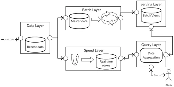
3.3 Lambda Architecture . . . 31
3.3.1 Batch Layer . . . 32
3.3.3 Speed Layer . . . 33
3.3.4 Data and Query layers . . . 34
3.3.5 Lambda Architecture Layers . . . 35
3.3.6 Recovery Mechanism . . . 35
3.4 Apache Beam . . . 36
3.4.1 Google Cloud Dataflow Architecture . . . 37
3.4.2 Processing Guarantees . . . 37
3.4.3 Strong and Weak Production Mechanisms . . . 38
3.4.4 Apache Beam Runners . . . 39
4 Comparative Analysis 41 4.1 Windowing Mechanism . . . 41
4.2 Processing and Result Guarantees . . . 44
4.3 Fault Tolerance Mechanism . . . 45
4.4 Strengths and Weaknesses . . . 45
5 Experiments and Results 47 5.1 Experimental Setup . . . 47
5.2 Apache Kafka Configuration . . . 48
5.3 Processing Pipelines . . . 48
5.4 Apache Spark . . . 50
5.4.1 Processing Time . . . 51
5.4.2 The Accuracy of Results . . . 54
5.4.3 Different Kafka Topics . . . 56
5.4.4 Different Processing Pipelines . . . 56
5.5 Apache Flink . . . 57
5.5.1 Running Modes . . . 57
5.5.2 Buffer Timeout . . . 58
5.5.3 The Accuracy of Results . . . 58
5.5.4 Processing Time of Different Kafka Topics . . . 60
5.5.5 Processing Time of Different Pipelines . . . 61
5.6 Apache Beam . . . 62 5.6.1 Spark Runner . . . 62 5.6.2 Flink Runner . . . 63 5.7 Discussion . . . 63 5.8 Future Work. . . 63 6 Conclusion 67 References 70 A Source Code 75
2.1 Two phase commit protocol . . . 6
2.2 Consensus problem . . . 8
2.3 Paxos algorithm message flow . . . 10
2.4 Raft state diagram . . . 12
2.5 Raft sequence diagram . . . 13
2.6 Zab protocol. . . 16
2.7 Zab protocol in ZooKeeper . . . 17
2.8 ZooKeeper hierarchical namespace. . . 18
2.9 Apache Kafka architecture . . . 21
3.1 Flink stack. . . 27
3.2 Lambda architecture . . . 35
3.3 Dataflow strong production mechanism . . . 39
3.4 Dataflow weak production mechanism. . . 40
4.1 Spark stream processing pipeline . . . 42
4.2 Flink stream processing pipeline . . . 42
4.3 Apache Beam stream processing pipeline . . . 43
5.1 Processing pipeline . . . 49
5.2 Arrival-time stream processing pipeline . . . 50
5.3 Session stream processing pipeline . . . 51
5.4 Event-time stream processing pipeline. . . 52
5.5 Number of processed records per second for different number of batches 52 5.6 Spark execution time for different number of batches . . . 53
5.7 Spark execution time for each micro-batch . . . 53
5.8 Spark execution time withReliable Receiver . . . 54
5.9 Network partitioning classes . . . 55
5.10 Spark execution time with different Kafka topics . . . 56
5.11 Spark execution time with different processing pipelines . . . 57
5.12 Flink execution time of both batch and streaming modes . . . 58
5.13 Flink execution time with different buffers in batch mode . . . 59
5.14 Flink execution time with different buffers in streaming mode. . . 59
5.15 Flink execution time with different Kafka topics . . . 61
5.16 Flink execution time with different processing pipelines . . . 61
5.17 Flink execution time with event-time pipeline . . . 62
4.1 Available windowing mechanisms in the selected stream processing engines . . . 44
4.2 The accuracy guarantees in the selected stream processing engines . . 45
5.1 The versions of the used frameworks . . . 47
5.2 Different Kafka configurations . . . 48
5.3 Different Kafka topics . . . 48
5.4 The accuracy of results with Spark and Kafka when failures happen . 54
Introduction
There are various sensors through which data is gathered by many approaches such as smart devices, satellites, and cameras. These sensors generate a huge amount of data that needs to be stored, processed, and analyzed. There are organizations that collect data for different reasons such as research, market campaigns, different trends detection in stock market, and describing a social phenomenon around the world. These organizations consider the data as the new oil1. If data becomes too big, it will be difficult to extract useful information out of it using a regular computer. Such amount of data needs considerable processing power and storage capacity.
1.1
Big Data Processing
There are two approaches to solve the problem of Big Data processing. The first approach is to have a single computer with very high-level computational and storage capacity. The second approach is to connect many regular computers together and building a cluster of computers. In the subsequent approach, storage capacity and processing power are distributed among regular computers. Configuring and managing clusters is a complex process because cluster management has to handle many aspects while dealing with Big Data Systems such as scalability, fault tolerance, robustness, and extensibility.
Due to the high number of components used within Big Data processing systems, it is likely that individual components will fail under any circumstances. This kind of systems face many challenges to deliver robustness and fault tolerance. Therefore, usually data sets should be immutable. Big Data systems should have the already processed data and not just an event state to facilitate recomputing the data when needed. Additionally, component failures can cause some data sets to be unavailable. Thus, data replication on distributed computers is needed [1].
Furthermore, Big Data processing systems should have the ability to process a variety types of data. They should be extensible systems by allowing the integration of new functionalities and supporting other types of data at a minimal cost [2]. Moreover, these systems have to be able to either scale-up or scale-out while data
is growing rapidly [1]. There are two kinds of frameworks which can handle these clusters: Batch processing and Stream processing.
1.1.1
Batch Processing
Batch processing frameworks process Big Data across a cluster of computers. They consider that data has already been collected for a period of time to be processed. Google has innovated a programming model called MapReduce for batch processing frameworks. This model takes the responsibility of distributing Big Data jobs on a large number of nodes. Also, it handles node failures, inter-node communications, disk usage and network utilization. Developers need only to write two functions (Map and Reduce) without any consideration of resource and task allocation. This
model consists of a file system, a master node, and data nodes [3].
The file system splits the data into chunks, after which it stores the data chunks in a distributed manner on cluster nodes. The master node is the heart of MapReduce model because it keeps track of running jobs and existing data chunks. It has access to meta-data that contains the locations of each data chunk. The data node, called a worker as well, handles storing data chunks and running MapReduce tasks. The worker nodes report to the master node periodically. As a result, the master node becomes able to know which worker nodes are still up, running and ready for performing tasks. If a worker node fails while processing a task, the master node will assign this task to another worker node. Thus, the model becomes fault tolerant [3]. One of the implementations of MapReduce Model is Apache Hadoop2.
The number of running computers on the cluster and the data-set size are the key parameters that determine the execution time of a batch processing job. It may take minutes, hours or even days [1, 4]. Therefore, batch processing frameworks have high latency to process Big Data. As a result, they are inappropriate to satisfy real-time constraints [5].
1.1.2
Stream Processing
Stream processing is a model for returning results in a low latency fashion. It addresses the high latency problem of the batch processing model. In addition, it includes most of batch processing features such as fault tolerance and resource utilization. Unlike batch processing frameworks, stream processing frameworks target to process data that is collected in a small period of time. Therefore, stream data processing should be synchronized with the data flow. If a real-time system requires X+1 minutes to process data sets which are collected in X minutes, then this system may not keep up with the data volumes and the results may become outdated [6].
Furthermore, storing data in such frameworks is usually based on windows of time, which are unbounded. If the processing speed is slower than the data flow speed, time windows will drop some data when they are full. As a result, the system becomes inaccurate because of missing data [7]. Therefore, all time windows should
have the potential to accommodate variations in the speed of the incoming and outgoing data by being able to slide as and when required [8].
In case of network congestion, real-time systems should be able to deal with delayed, missing, or out-of-order data. They should guarantee predictable and repeatable results. Similar to batch processing systems, real-time systems should produce the same outcome having the same data-set if the operation is re-executed later. Therefore, the outcome should be deterministic [8].
Real-time stream processing systems should be up and available all the time. They should handle node failure because high availability is an important concern for stream processing. Therefore, the system should replicate the information state on multiple computers. Data replication can increase the data volumes rapidly. In addition, Big Data processing systems should store the previous and the recent results because it is common to compare them. Therefore, they should be able to scale-out by distributing processing power and storage capacity across multiple computers to achieve incremental scalability. Moreover, they should deal with scalability automatically and transparently. These systems should be able to scale without any human interaction [8].
1.2
Problem Statement
The batch processing model is able to store and process large data sets. However, this model becomes no longer enough for modern businesses that need to process data at the time of its creation. Many organizations require to process data streams and produce results in low latency to make faster and better decisions in real time. These organizations believe that data is more valuable at the time of generation and data would loss its value over time.
Stream processing systems need to provide the benefits of the batch processing model such as scalability, fault tolerance, processing guarantees, and the accuracy of results. In addition, these systems should process data at the time of its arrival. Due to network congestion, server crashes, and network partitions, some data may be lost or delayed. Consequently, some data might be processed many times, which influences the accuracy of results.
This thesis provides a comparative analysis of selected stream processing frame-works namely Apache Spark, Apache Flink, Lambda Architecture, and Apache Beam. The goal of this research is to provide a clear and fair comparison of the selected frameworks in terms of data processing methodologies, data processing guarantees, and the accuracy of results. In addition, this thesis examines how these frameworks interact with external sources of data such as HDFS and Apache Kafka.
1.3
Thesis Structure
The rest of the thesis is organized as follows. Chapter 2 discusses selected fault tolerance mechanisms which are used in Big Data systems. Chapter3 explains the architecture of the following stream processing frameworks: Apache Spark, Apache
Flink, Lambda Architecture, and Apache Beam. Chapter 4provides a comparative analysis of the discussed frameworks from different perspectives such as available functionalities, windowing mechanism, processing and result guarantees, and fault tolerant mechanism. Chapter5shows results of experiments on some of the discussed frameworks to emphasis their strengths and weaknesses. The experiments examine the following: the processing time, processing guarantees and the accuracy of results in case of failures of each framework. Furthermore, this chapter discusses the findings of the experiments and possible future extensions. The last chapter provides a summary of what we have achieved.
Fault Tolerance Mechanisms
Scalability and data distribution have an impact on data consistency and availability. Consistency guarantees that storage nodes hold identical data element for same data chunk at a specific time. Availability guarantees that every request receives a response about whether it succeeded or failed. Availability is affected by component failures such as computer crashes or networking device failures. Networking devices are physical components, which are responsible for interaction and communication between computers on a network1. These components may fail, after which the network is split into sub-networks causing network partitioning.
While distributing data among different storage nodes over the network, it is common to have network partitions. As a result, some data may become unavailable for a while. Partition tolerance guarantees that the system continues to operate despite network partitioning2. Data replication over multiple storage nodes greatly alleviates this problem [9]. However, if data is replicated in ad-hoc fashion, it can lead to data inconsistency [10].
2.1
CAP Theorem
E. Brewer [11] identifies the fundamental trade-off between consistency and availabil-ity in a theorem called the CAP theorem. This theorem concerns what happens to data systems when some computers can not communicate with each other within the same cluster. It states that when distributing data over different storage nodes, the data system becomes either consistent or available but not both during the network partitioning. It prohibits perfect both consistency and availability at the same time in the presence of network partitions.
The CAP theorem forces system designers to choose between availability and consistency. The availability focuses on building an available system first and then trying to make it as consistent as possible. This model can lead to inconsistent states between the system nodes which can cause different results on different computers. However, it makes the system available all the time. On the other
1https://en.wikipedia.org/wiki/Networking_hardware 2https://en.wikipedia.org/wiki/CAP_theorem
hand, the consistency focuses on building a consistent state first and then trying to make it as available as possible. This model can lead to unavailable system when network partitions. It guarantees that a system has identical data when the system is available.
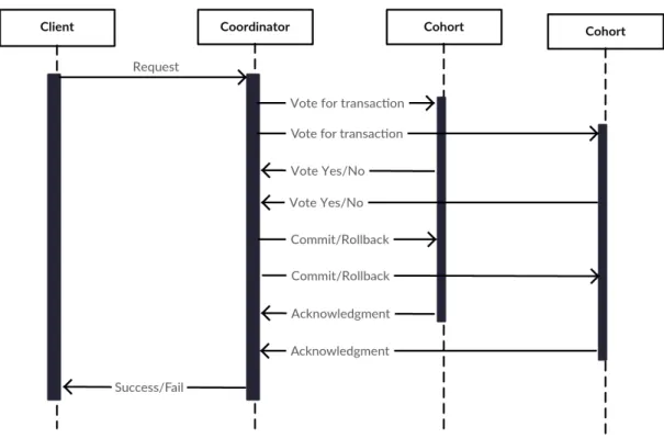
Consistent systems ensure that each operation is executed on all computers. There are many protocols to build a consistent system such as Two phase commit protocol [12]. This protocol targets having an agreement from all computers, involved in the operation, before performing that operation. It relies on a coordinator node, which is the master node, to receive client’s requests and coordinate with other computers called cohorts. The coordinator discards the operation if one of the cohorts fails or does not respond. Figure 2.1depicts how two phase commit protocol works. Reaching the agreement for thecommit phase is straightforward if the network and participating computers are reliable. However, this is not always the case in distributed systems due to computer crashes and network partitions.
The two phase commit protocol does not work under arbitrary node failures because the coordinator is a single point of failure. If the coordinator fails, it becomes unable to receive client’s requests. Moreover, if the failure happens after the voting phase, cohorts might be blocked because they will be waiting for either a commit or rollback message. Thus, the two phase commit protocol is not fault tolerant.
Available systems try to execute each operation on all computers. They keep running if some computers are unavailable. These systems manage network partitions in three steps. Firstly, the system should detect that there is a partition. Secondly, it should deal with this partition by limiting some functionalities, if necessary. Finally, it should have a recovery mechanism when the partition no longer exists. When the partition ends, the recovery mechanism makes all system computers consistent, if possible.
There is not any unified recovery approach that works for all applications while having an available system and network partitions. The recovery approach depends on the available functionalities on each system when the network partitions [11]. For example, Amazon Dynamo [13] is a highly available key-value store. This service targets the following goals: high scalability, high availability, high performance, and low latency. It allows write operations after one replica has been written. Therefore, data may have multiple versions. The system tries to reconcile them. If the system cannot reconcile them, it asks the client for reconciliation in an application specific manner.
2.2
FLP Theorem
In distributed systems, it is common to have failed and slow processes which receive delayed messages. It is impossible to distinguish between them in a fully asynchronous system, which has no upper bound on message delivery. Michael J. Fischer et al. [14] prove that there is no algorithm that will solve the asynchronous consensus problem in a theory called the FLP theorem.
Consensus algorithms can have an unbounded run-time, if a slow process is repeatedly considered to be a dead process. In this case, consensus algorithms will not reach a consensus and they will run forever. For example, Figure 2.2 depicts this problem when having a dead or a slow process in a system. ProcessA wants to reach a consensus for an operation, therefore it sends requests to other processesB, C, and D. ProcessD is slow and Process C is already dead. Although, Process A
considers ProcessD as a dead process as well. As a result, Process A will not reach a consensus. The FLP theorem states that this problem can be tackled if there is an upper bound on transmission delay. Furthermore, an algorithm can be made to solve the asynchronous consensus problem with very high probability to reach a consensus.
2.3
Distributed Consensus
Instead of building a completely available system, a consensus algorithm is used to build a reasonably available and consistent system. Consensus algorithms, such as Paxos [15], Raft [16], and Zab [17], aim at reaching an agreement from the majority of computers. They play a key role in building highly-reliable large-scale distributed systems. These kinds of algorithms can tolerate computer failures. Consensus algorithms help a cluster of computers to work as a group which can survive even when some of them fail.
Figure 2.2: Consensus problem
The importance of consensus algorithms arises in the case of replicated state machines [18]. This approach aims to replicate identical copies of a state machine on a set of computers. If a computer fails, the remaining set of computers still have identical state machine. Such a state machine can, for example, represent the state of a distributed database. This approach tolerates computer failures and is used to solve fault tolerance problems in distributed systems. Replicated state machines are implemented using a replicated log. Each log stores the same sequence of operations which should be executed in order. Each state machine processes the same operations in the same order. Consensus algorithms are used to keep the replicated log in a consistent state.
To ensure the consistency through a consensus algorithm, a few safety requirements must be held [19]. If there are many proposed operations from different servers, only one operation is chosen, out of them, at a time. Moreover, each server knows the chosen operation only when it has already been chosen. There are a few assumptions which are considered. Firstly, servers operate at different speeds. Secondly, messages can take different routes to be delivered which affect the communication time. Thirdly, messages can be duplicated or lost but not corrupted. Finally, all servers may fail after an operation has been chosen without other servers knowing it. As a result, these servers will never know about these operations after they are restarted. Consensus algorithms require that a majority of servers are up and able to communicate with each other to guarantee commitment of writes.
2.3.1
Paxos Algorithm
The Paxos algorithm [15] guarantees a consistent result for a consensus if it terminates. Therefore, this algorithm follows the FLP theorem because it may not terminate. It is used as a fault tolerance mechanism. It can tolerate n faults when there are2n+1
processes. If the majority, which is n+1 processes, agreed on an operation, then this operation can be performed.
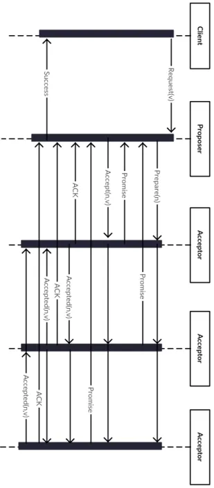
The Paxos algorithm has two operator classes: proposers and acceptors. Proposers are a set of processes which propose new operations called proposals. Acceptors are a set of processes which can accept the proposals. A single process may act as a proposer and an acceptor. A proposal consists of a tuple of values {a number, a proposed operation}. The Paxos algorithm requires the proposal’s number to be unique and totally ordered among all proposals. It has two phases to execute an operation: choosing an operation and learning it to others [19]. Figure 2.3depicts the message flow for a client request in a normal scenario.
2.3.1.1 Choosing an Operation
The Paxos algorithm requires the majority of acceptors to accept a proposal before choosing it. The algorithm wants to guarantee that if there is only one proposal, it will be chosen. Therefore, acceptors must accept the first proposal that they receive. However, different acceptors can accept different proposals. As as result, no single proposal will be accepted by the majority. Acceptors must be allowed to accept more than one proposal but with additional requirement.
Many proposals can be accepted if they have the same operation. If a proposal with a tuple{n,v} is chosen, then every proposal with proposal’s number greater than n
should have the same operation v. All acceptors must guarantee this requirement. Therefore, if a proposal is chosen, every proposal with a higher number than the chosen one must have the same operation. However, if an acceptor fails and then it is restarted, it will not know the highest-numbered chosen proposal. This acceptor must accept the first proposal it receives. The Paxos algorithm transfers the responsibility of knowing the chosen proposal with the highest number from the acceptors side to the proposers side. Each proposer must learn the highest-numbered proposal in order to issue a new proposal. Consequently, the Paxos algorithm guarantees that:
For each set of acceptors, if a proposal with a tuple {n,v} is issued, then it is guaranteed that either no acceptor has accepted any proposal with a number less thannor the operationv is same as the highest-numbered chosen proposal.
The Paxos algorithm follows two phases for choosing an operation. Firstly, a proposer must prepare for issuing a new proposal. It should send a prepare request to each acceptor. This request consists of a new proposal with numbern. It asks for a promise not to accept any proposal with number less thann. Moreover, it asks for the highest-numbered proposal that has been accepted, if there. When an acceptor receives a prepare request with numbern that is greater than of any prepare requests to which it has already responded, it responds with a promise not to accept any
Figure 2.3: Paxos algorithm message flow
proposals with numbers less than n. Additionally, the acceptor may send the highest-numbered proposal that it has accepted.
Secondly, if the proposer receives responses from the majority of acceptors, then it issues a proposal with the number n and an operation v. The operation v is either same as the highest-numbered proposal from one of the acceptors, or any operation if the majority reported that there is no accepted proposals. The proposer sends an accept request to each of those acceptors with the issued proposal. If an acceptor receives an accept request for a proposal with number n, it accepts the proposal
unless it has already responded to another prepare request with greater number than n. This approach guarantees that if a proposal with an operation v is chosen, then every higher-numbered proposal, issued by any proposer, must have the same operationv. However, there is a scenario that prevents accepting any proposal.
Assume that there are two proposers p and q. Proposerp has issued a proposal with numbern1. While proposerqhas issued a proposal with numbern2wheren2>n1.
Proposer p got a promise from the majority of acceptors that they will not accept any proposals with number less than n1. Then, proposal q got a promise from
the majority of acceptors that they will not accept any proposals with number less thann2. Sincen1<n2, the acceptors will deny accepting the proposal with numbern1
after their promise to proposer q. This problem causes no progress in issuing and accepting proposals. The Paxos algorithm elects one server to be the only proposer in the system at a time to solve this problem. This proposer will send prepare and
accept requests to acceptors. However, this approach can affect the liveness of the system if only one proposer has a lock forever. This problem can be tackled by setting a timeout for each lock, which the lock is released.
2.3.1.2 Learning a Chosen Operation
After issuing proposals and choosing an operation, acceptors must know that a pro-posal has been accepted by the majority to be performed. When an acceptor accepts a proposal, it informs other acceptors. When an acceptor receives an accepted proposal from the majority of acceptors, it becomes able to perform the operation of the chosen proposal.
Due to message loss and server crashes, a proposal could be chosen and an acceptor will never know about it. Acceptors can ask each other about the accepted proposals. However, failures of multiple acceptors at the same time can prevent an acceptor to know whether a proposal has been accepted by the majority. In this case, the acceptor will never know about the chosen proposal unless a new one has been issued. As a result, acceptors will inform each other about the accepted proposals. Thereby, this acceptor will find out the chosen operation by the majority.
One of the Paxos algorithm usages is to perform operations on a cluster of computers. All computers should perform the operations in the same order. As a result, their state machines become identical. The Paxos algorithm is used for implementing identical state machines on distributed computers.
2.3.1.3 Implementing a State Machine
The straightforward way to implement a distributed system is by sending all requests to a central server, after which this server broadcasts them to other servers in a specific order. This central server acts as a proposer to guarantee better progress of proposals. However, this server becomes a single point of failure. Therefore, the Paxos algorithm considers that each server is able to act as proposer and acceptor. However, practical Paxos implementations select a single proposer with a leader election algorithm.
The leader becomes the only proposer in the system. It receives requests and organizes them in order. The Paxos algorithm guarantees the order of requests by
proposal’s numbers. For each request, the leader issues a new proposal with a number greater than the issued proposals. Then, it sendsprepareandaccept requests to other servers. When the leader fails, a new leader is elected. The new leader may have some missing proposals. The leader tries to fill them by sending aprepare request for each missing proposal. The leader cannot consider new requests before filling the gaps. If there is a gap that should be filled immediately, the leader sends a special request that leaves the state machine unchanged.
2.3.2
Raft Algorithm
The Paxos algorithm has proven its efficiency, safety, and liveness. Nonetheless, it has shown to be fairly difficult to understand [16]. Also, it does not have a unified approach for implementation. The Raft algorithm [16] is similar to the Paxos algorithm but is easier to understand by having a more straightforward approach.
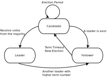
The Raft algorithm has three different states for servers: leader,follower, and can-didate. Only one server can act as a leader at a time, and other servers are followers. The leader receives client’s requests and sends them to the followers. Followers respond to the leader’s requests without issuing any of them. If a follower receives a client’s request, it passively redirects the request to the leader. The leadership lasts for a period of time called term. Figure 2.4 presents the cases how servers are changing their states.
Figure 2.4: Raft state diagram
The Raft algorithm divides the running time into terms which are numbered in an ascending order. The duration of the terms is random, after which terms will expire. Each term has a leader which receives all requests, and stores them in a local log. Then, it sends them to the followers. If a server discovers that it has a smaller term number, the server updates its term number. On the other hand, if a server discovers that it has a higher term number, it rejects the request. If a leader or a candidate discovers that its term number is out-of-date, it converts itself to a follower state. Term numbers are exchanged between servers while communicating.
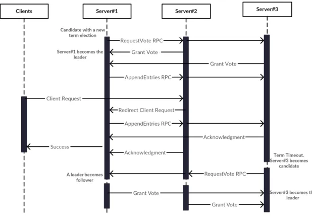
Communication between Raft cluster is based on RPCs. There are two types of RPCs:RequestVote andAppendEntries. RequestVote RPCs are used at the beginning of a term for electing a new leader. AppendEntries RPCs are used to send requests to followers. Figure2.5 describes how the Raft algorithm works in normal scenario. Leader’s requests are new logs to be appended or heartbeats to keep the leadership.
Figure 2.5: Raft sequence diagram
2.3.2.1 Leader election
When there is no leader, all servers go to the candidate state for electing a new leader with a new term number. If a candidate wins, it acts as a leader for rest of the term. If electing a leader fails, a new term will start with a new leader election. When a leader is elected and as long as followers are receiving valid RPCs, they remain in the follower state.
When a follower does not receive any RPCs for a specific period of time called elec-tion timeout, the follower changes its state to a candidate state. It increases the current term number for a new leader election. Then, it issues RequestVote RPCs to all servers for voting itself as a new term leader. A candidate has three scenarios which can happen after voting for a new leadership.
Firstly, a candidate wins an election if it receives acceptance votes from the majority of servers. Each server votes at most once in each term. Servers follow First-Come-First-Serve(FCFS) approach while accepting votes. Choosing a leader by the majority of servers ensures that at most one candidate will be elected as a leader.
Once a candidate is elected to be the term leader, it receives client requests and sends AppendEntries RPCs to other servers.
Secondly, while a candidate is waiting for votes, it may receive an AppendEntries
RPC from another leader term. If the RPC’s term number is larger than the candidate’s term number, then the candidate converts its state to a follower state and updates its current term to the leader’s term number. If the candidate receives the RPC with a smaller term number, the candidate rejects it and continues in the candidate state.
Finally, if a candidate neither wins nor loses, it will start a new vote after the election timeout. This can happen because many followers become candidates at the same time. As a result, each one votes to be a leader at the same time with no progress. The Raft algorithm uses randomized election timeout to ensure that having such scenario is rare. The random election timeout for each candidate ensures that this problem will never happen in two terms respectively.
Raft has a restriction in electing a new leader. The new leader should be up-to-date with the majority of candiup-to-dates. The voting process prevents electing a leader that has less log entries. When a candidate votes itself, it sends RequestVote RPCs to all candidates. Each RequestVote RPC contains the following fields:
• Term: The candidate’s new term number, which is the last term + 1.
• Candidate Id: The id of the candidate which is requesting vote.
• Last Log Index: The candidate sends its last log index, so that other candidates can check whether this candidate has at least what they have in their logs.
• Last Log Term: This is the term number for the last log index. This helps other candidates to check whether the last index belongs to a correct term number according to their logs.
The receiver candidate grants vote if its log is at least up-to-date to the sender candidate’s log. If the receiver candidate has more entries than the sender candidate or it has already voted to another candidate, it replies through an RPC with a rejection response.
2.3.2.2 Log Replication
Once a leader is elected, it manages client’s requests. Each client request contains an operation to be committed in the state machine. Once the leader receives a request, it stores the request’s operation in the local log as a new entry. Then, it creates
AppendEntries RPCs in parallel for each follower in the Raft cluster. When the majority of followers adds the RPCs to their logs, the leader executes the operation to its state machine and returns the result to the client. The executed operation is called committed. The leader tells followers about the committed entries when sendingAppendEntries RPCs. If some followers do not acknowledge an RPC message due to slow process, message loss, or server crashes, the leader retries sending the
RPC until all servers become eventually synchronized. The Raft algorithm follows a specific methodology to ensure consistency between all servers.
Each log entry consists of a term number, an operation, and an index. The index must be identical on all servers. The leader sorts and manages the indexes of the log entries. Moreover, it keeps track of the last committed log entry. It distributes the log entries via RPCs. Each AppendEntries RPC consists of the following:
• Term: This is the current term number. Followers use it to detect fake leaders and make sure of consistency.
• Leader Id: Followers use this id to redirect client’s requests to the leader, if there.
• Previous Log Index: Followers use this index to make sure that there are not any missing entries and they are consistent with the leader.
• Previous Log Term: Followers use it to make sure that the previous log index belongs to the same term number. This is useful when a new leader is elected. Followers can ensure consistency.
• Array of entries: This array consists of a list of ordered entries which followers should add them to their logs. In case of HeartBeat RPCs, this field is empty.
• Leader Commit: This field contains the last committed log index. Followers use this field to find out which operations should be executed to their state machines.
Followers reply to theAppendEntries RPCs by another RPC to inform the leader whether the log entries are added. This RPC reply is essential in case of leader failure.
A leader can fail after adding entries to its log without replicating them. Also, it can fail after committing a set of operations to its state machine without informing others. When a new leader is elected, it handles inconsistencies. The leader forces the followers to follow its log; the leader never overrides its log. When the leader sends
AppendEntries RPCs to followers with a specific Previous Log Index, it waits for a result RPC from each follower. If the leader receives a failure RPC from a follower, it recognizes that they are inconsistent. Therefore, it sends anotherAppendEntries
RPC to this follower but with less Previous Log Index. The leader keeps decreasing this index until the follower eventually succeeded. The follower removes all log entries after the succeeded index. The leader sends all log entries after that index. Therefore, they become in a consistent state.
2.3.3
Zab Algorithm
The original Paxos algorithm requires that if there is an outstanding operation, all issued proposals should have the same operation. Therefore, it does not enable multiple outstanding operations. The Zab algorithm [17] is used as an atomic broad-cast algorithm. Unlike the Paxos algorithm, it guarantees total delivery operations
order based on First-In-First-Out (FIFO) approach. It assumes that each operation depends on the previous one. It gives each operation astate change number that is incremented with respect to the state number of the previous operation. The Zab algorithm assumes that each operation is idempotent; executing the same operation multiple times does not lead to an inconsistent state. Therefore, it guaranteesexactly once semantics.
The Zab algorithm elects a leader to order client’s requests. Figure 2.6 describes the phases of Zab protocol. After the leader election phase, a new leader starts a new phase to discover the highestidentification schema. Then, the leader synchronizes its log with the discovered highest schema. After being up-to-date, the leader starts to broadcast its log to other servers. The Zab algorithm follows a different mechanism than the Raft algorithm in case of recovering leader failures.
Figure 2.6: Zab protocol3
The recovery mechanism is based on identification schema that enables the new leader to determine the correct sequence of operations to recover state machines. Unlike the Raft algorithm, the new leader updates its log entries. Additionally, it is not mandatory for the new leader to be up-to-date. Each operation is identified by the identification schema and the position of this operation in its schema. Only a server with the highest identification schema can send the accepted operations to the new leader. Thereby, only the new leader is responsible for deciding which server is up-to-date using the highest schema identifier.
Communication between different servers is based on bidirectional channels. The Zab algorithm uses TCP connections to satisfy its requirements about integrity and delivery order. Once the new leader recovers the latest operations, it starts to establish connections with other servers. Each connection is established for a period of time called iteration. The Zab algorithm is used in Apache Zookeeper4 to implement
a primary-backup schema.
2.4
Apache ZooKeeper
Apache ZooKeeper [20] is a high-performance coordination service for distributed systems. It enables different services such as group messaging and distributed locks in a replicated and centralized fashion. It aims to provide a simple and high performance coordination kernel for building complex primitives.
3http://www.tcs.hut.fi/Studies/T-79.5001/reports/2012-deSouzaMedeiros.pdf 4https://zookeeper.apache.org/- A coordination distributed service
Instead of implementing locks on primitives, ZooKeeper implements its services based on wait-free data objects which are organized in hierarchy similar to file systems. It guarantees FIFO ordering for client operations. It implements the ordering mechanism by following a simple pipelined architecture that allows buffering many requests. The wait-free property and FIFO ordering enable efficient implementation for performance and fault tolerance.
ZooKeeper uses replication to achieve high availability through comprising of a large number of processes to manage all coordination aspects. It uses the Zab algorithm to implement a leader-based broadcast protocol for coordinating between different processes. The Zab algorithm is used in update operations but it is not used in read operations because ZooKeeper servers manage them locally. It guarantees consistent hierarchical namespace among different servers. However, ZooKeeper implements the Zab protocol in a different way3. Figure 2.7shows the phases that
are implemented. ZooKeeper combines Phases 0 and 1 of the original Zab protocol in a phase called Fast Leader Election. This phase attempts to elect a leader that has the most up-to-date operations in its log. Thereby, the new leader does not need the Discovery phase to find the highest identification schema. The new leader needs to recover the operations to broadcast. These operations are organized in hierarchical namespaces.
Figure 2.7: Zab protocol in ZooKeeper3
ZooKeeper manages data nodes according to hierarchical namespaces called data trees. There are two types of data nodes, which are called znodes:
• Regular znodes: Clients manage to create and delete them explicitly,
• Ephemeral znodes: Clients create this type of znodes. Clients can either delete them explicitly or the system removes them when the client’s session is terminated.
Data trees are based on UNIX file system paths. Figure 2.8 depicts the hierarchical namespace in ZooKeeper. When creating a new znode, a client sets a monotonically increasing sequential value. This value must be greater than the value of the parent znode. Znodes under the same parent znode must have unique values. As a result, ZooKeeper guarantees that each znode has a unique path which clients can use to read data.
When a client connects to ZooKeeper, the client initiates a session. Each session has a timeout, after which ZooKeeper terminates the session. If the client does not send any requests for more than the timeout period, the ZooKeeper service
Figure 2.8: ZooKeeper hierarchical namespace
considers it as a faulty client. While terminating a session, ZooKeeper deletes all ephemeral znodes related to this client. During the session, clients use an API to access ZooKeeper services.
Client API: ZooKeeper exposes a simple set of services in a simple interface which clients can use for several services such as configuration management and synchronization. The client API enables clients to create and delete data within a specific path. Moreover, clients can check whether a specific data exists, in addition to changing and retrieving this data.
Clients can set a watch flag when requesting a read operation on a znode to be notified if the retrieved data has been changed. ZooKeeper notifies clients about changes without the need of polling the data itself again. However, if data is big, then managing flags and data change notifications may consume a reasonable amount of resources and need larger latency. Therefore, ZooKeeper is not designed for data storage. It is designed for storing meta-data information or configuration about the data itself. Clients can access only data trees which they are allowed to.
ZooKeeper manages access rights with each sub-tree of the data tree using a hierarchical namespace. Clients have the ability to control who can access their data. Additionally, ZooKeeper implements the client API in both synchronous and asynchronous fashion. Clients use the synchronous services when they need to perform one operation to ZooKeeper at a time. While they use the asynchronous services when they need to perform a set of operations in parallel. ZooKeeper guarantees that it responds to the corresponding callbacks for each service in order.
ZooKeeper guarantees a sequential consistency, timeliness, atomicity, reliability, and single image view. The sequential consistency is guaranteed by applying the operations in the same order which they were received by the leader. Atomicity of transaction is guaranteed by each action either succeeding or failing. ZooKeeper can be configured to guarantee that any server has the same data view. In addition, it guarantees the reliability of updates by making sure that once an update operation is persisted, the update effect remains until overriding it. One of the systems which uses ZooKeeper is Apache Kafka5.
2.5
Apache Kafka
Apache Kafka [21] is a publisher-subscriber, distributed, scalable, partitioned and replicated log service. It offers a high throughput messaging service. It aims to store data in real time by eliminating the overhead of having rich delivery guarantees. Kafka consists of a cluster of servers, each of which is calledbroker. Brokers maintain feeds of messages in categories called topics. A topic is divided into partitions for load balancing. Partitions are distributed among brokers. Each partition contains a sequence of messages. Each message is assigned a sequential id number calledoffset, which is unique within its partition. Clients add messages to a topic throughproducers
and they read the produced messages through consumers.
For each topic, there is a pool of producers and consumers. Producers publish messages to a specific topic. Consumers are organized inconsumer groups. Consumer groups are independent and no coordination is required among them. Each consumer group subscribes to a set of topics and creates one or more message streams. Each message stream iterates over a stream of messages. Message streams never terminate. If there is no more messages to be consumed, the message stream’s iterator blocks consuming until new messages are produced. Kafka offers two consumption delivery models: point-to-point and publish/subscribe. In point-to-point model, a consumer group consumes a single copy of all messages in a topic. In this model, Kafka delivers each message to only one consumer for each consumer group. In publish/subscribe model, each consumer consumes all the message in a topic. Consumers can only read messages sequentially. This allows Kafka to deliver messages in high throughput through a simple storage layer.
The simple storage layout helps Kafka to increase its efficiency. Kafka stores each partition in a list of logical log files, each of which has the same size. When a producer produces a message to a topic, the broker appends this message to the end of the current log file of the corresponding partition. Kafka flushes files after a configurable number of time for better performance. Consumers can only read the flushed messages. If a consumer acknowledges that it has received a specific offset, this acknowledgement implies that it has received all messages prior to that offset. Kafka does not support random access because messages do not have explicit message ids but instead have logical offsets. Brokers manage partitions in a distributed manner.
Each partition has a leader broker which handles all read and write requests to that partition. Partitions are designed to be the smallest unit of parallelism. Each partition is replicated across a configurable number of brokers for fault tolerance. Partitions are consumed by one consumer within each consumer group. This approach eliminates the needs of coordination between different consumers within the same consumer group to know whether a specific message is consumed. Moreover, it eliminates the needs of managing locks and state maintenance overhead which affect the overall performance. Consumers within the same consumer group need only to coordinate when re-balancing the load of consuming messages.
Consumers read messages by issuing asynchronous poll requests for a specific topic and partition. Each poll request contains a beginning offset for the message consumption in addition to number of bytes to fetch. Consumers receive a set of
messages from each pull request. Kafka implements a consumer API for managing requests. The consumer API iterates over the pulled messages to deliver one message at a time. Consumers are responsible for specifying which offsets are consumed. Kafka gives consumers more flexibility to read same offsets more than once. It designs brokers to be stateless.
Brokers do not maintain the consumed offsets for each consumer. Therefore, they become blind of the consumed messages to be deleted. Kafka has a time-based SLA for message retention. After a configurable time of producing a message, Kafka automatically deletes it. However, Kafka enables storing data forever. This approach reduces the complexity of designing brokers and utilizes the performance of message consumption. Additionally, Kafka utilizes the network consumption while producing messages. It allows producers to submit a set of messages in a single send request. Furthermore, It utilizes brokers’ memory by avoiding caching messages in memory. Instead, it uses the file-system page cache. When a broker restarts, it retains the cache smoothly. This approach makes Kafka avoiding the overhead of the memory garbage collection. Moreover, Kafka avoids having a central master node for coordination. It is designed in a decentralized fashion.
Distributed Coordination:Figure 2.9describes Kafka components and how they use Apache ZooKeeper. Apache Kafka uses ZooKeeper to coordinate between different system components as following:
• ZooKeeper detects the addition and the removal of brokers and consumers. When a new broker joins Kafka’s cluster, the broker stores its meta-data information in a broker registry into ZooKeeper. The broker registry contains its host name, port, and partitions which it stores. Similarly, when a new consumer starts, it stores its meta-data information ina consumer registry into ZooKeeper. The consumer registry consists of the consumer group, which this consumer belongs to, and the list of subscribed topics.
• ZooKeeper triggers the re-balance process. Consumers maintain watch flags in ZooKeeper for the subscribed topics. When there is a change in consumers or brokers, ZooKeeper notifies consumers about this change. Consumers can initiate a re-balance process to determine the new partitions to consume data from. When a new consumer or a new broker starts, ZooKeeper re-balances the consumption over brokers to utilize the usage of all brokers.
• ZooKeeper maintains the topic consumption. It associates anownership registry
and anoffset registry for each consumer group. Theownership registry stores which consumer consumes which partition. The offset registry stores the last consumed offset for each partition. When a new consumer group starts and no
offset registry exists, consumers start consuming messages from either smallest or largest offset. When a consumer starts consuming from a specific partition, the consumer registers itself in the ownership registry as the owner of this partition. Consumers periodically update the offset registry with the last consumed offsets.
Kafka uses ephemeral znodes to create broker registries, consumer registries, and ownership registries. While it uses regular znodes to create offset registries. When a broker fails, ZooKeeper automatically removes its broker registry because this registry is no longer needed. Similarity, when a consumer fails, it removes its consumer registry. However, Kafka keeps the offset registry to prevent the consumption of the consumed offsets when a new consumer joins the same consumer group.
Stream Processing Frameworks
Batch processing frameworks need a considerable amount of time to process Big Data and produce results. Modern businesses require producing results in low latency. The demand for real-time access to information is increasing. Many frameworks have been proposed to process Big Data in real time. However, they face challenges, as discussed in Section1.1.2in processing data in low latency and producing results with high throughput. In addition, they face challenges in producing accurate results and dealing with fault tolerance. Unlike batch processing frameworks, stream processing frameworks collect records into data windows [22].
Data windows divide data-sets into finite chunks for processing as a group. Data windowing is required to deal with unbounded data streams. While it is optional to process bounded data-sets. A data window is either aligned or unaligned. Aligned window is applied across all the data for a window of time. Unaligned window is applied across a subset of the data from a window of time according to specific constraints such as windowing by key.
There are three types of windows when dealing with unbounded data streams1: fixed, sliding, and sessions. Fixed windows are defined by a fixed window size. They are aligned in most cases, however they are sometimes unaligned by shifting the windows for each key. Fixed windows do not overlap. Sliding windows are defined by a window size and a sliding period. They may overlap if the sliding period is less than the window size. A sliding window becomes a fixed window if the sliding period equals to the window size. Sessions capture some activities over a subset of data. If a session does not receive new records related to its activities for a period of time called a timeout, the session is closed.
Stream processing frameworks can process data according to its time domains such as event time and processing time. Event time domain is the time at which a record occurs or is generated. Processing time domain is the time at which a record is received within a processing pipeline. The best case for a record is when its event time equals to its processing time, but this is not the case in distributed systems. Apache Spark, Apache Flink, and Apache Beam are some of the frameworks that deal with Big Data stream processing.
3.1
Apache Spark
Apache Spark is an extension to the MapReduce model that efficiently uses cluster’s memory for data sharing and processing among different nodes. It adds primitives and operators over MapReduce to make it more general. It supports batch, streaming, and iterative data processing. Spark uses a memory abstraction model called Resilient Distributed Dataset [23] that efficiently manages cluster’s memory. Moreover, it implements Discretized Streams [24] for stream processing on large clusters.
3.1.1
Resilient Distributed Datasets
The MapReduce model lacks in dealing with applications which iteratively apply a similar function on the same data at each processing step such as machine learn-ing and graph processlearn-ing applications. These kinds of applications need iterative processing model. The MapReduce model deals badly with iterative applications because it stores data on hard drives and reloads the same data directly from hard drives on each step. MapReduce jobs are based on replicating files on distributed file system for fault recovery. This mechanism adds a significant overhead on network transmission when replicating large files. Resilient Distributed Dataset (RDD) is a fault-tolerant distributed memory abstraction that avoids data replication and minimizes disk seeks. It allows applications to cache data in memory across different processing steps which leads to substantial speedup on future data reuse. Moreover, RDDs can remember the operations used to build them. When a failure happens, they can re-build the data with minimal network overhead.
RDDs provide some restrictions on the shared memory usage for enabling low-overhead fault tolerance. They are designed to be read-only and partitioned. Each partition contains records which can be created through deterministic operations called transformations. Transformations include map, filter, groupBy, and join operations. RDDs can be created through other existing RDDs or a data set in a stable storage. These restrictions facilitate reconstructing lost partitions because each RDD has enough information about how to rebuild it from other RDDs. When there is a request for caching an RDD, Spark processing engine stores its partitions by default in memory. However, partitions may be stored on hard drives when enough memory space is not available or users ask for caching on hard drives only. Furthermore, Spark stores big RDDs on hard drives because they can never be cached to memory. RDDs may be partitioned based on a key associated with each record, after which they are distributed accordingly.
Each RDD consists of a set of partitions, a set of dependencies on parent RDDs, a computing function, and meta-data about its partitioning schema. The computing function defines how an RDD is built from its parent RDDs. For example, if an RDD represents an HDFS file, then each partition represents a block of the HDFS file. The meta-data will contain information about the HDFS file such as location and number of blocks. This RDD is created from a stable storage, therefore it does not have dependencies on parent RDDs. A transformation can be performed on some RDDs, which represent different HDFS files. The output of this transformation is
a new RDD. This RDD will consist of a set of partitions according to the nature of the transformation. Each partition will depend on a set of other partitions from the parent RDDs. Those parent partitions are used to recompute the child partition when needed.
Spark divides the dependencies on parent RDDs into two types: narrow and wide. Narrow dependencies indicate that each partition of a child RDD depends on a fixed number of partitions in parent RDDs such asmaptransformation. Wide dependencies indicate that each partition of a child RDD can depend on all partitions of the parent RDDs such as groupByKey transformation. This categorization helps Spark to enhance the execution and recovery mechanism. RDDs with narrow dependencies can be computed within one cluster node such as map operation followed by filter
operation. In contrast, wide dependencies require data from parent partitions to be shuffled across different nodes. Furthermore, a node failure can be recovered more efficiently with a narrow dependency because Spark will recompute a fixed number of lost partitions. These partitions can be recomputed in parallel on different nodes. In contrast, a single node failure might require a complete re-execution in case of wide dependencies. In addition, this categorization helps Spark to schedule the execution plan and take checkpoints.
Spark job scheduler uses the structure of each RDD to optimize the execution plan. It targets to build a Directed Acyclic Graph (DAG) of computation stages for each RDD. Each stage contains as many transformations as possible with narrow dependencies. A new stage starts when there is a transformation with wide dependencies or a cached partition that is stored on other nodes. The scheduler places tasks based on data locality to minimize the network communication. If a task needs to process a cached partition, the scheduler sends this task to a node that has the cached partition.
3.1.2
Discretized Streams
Spark aims to get the benefits of the batch processing model to build a streaming engine. It implements Discretized Streams (D-streams) model to deal with streaming computations. D-Streams model breaks down a stream of data into a series of small batches at small time intervals called Micro-batches. Each micro-batch stores its data into RDDs. Then, the micro-batch is processed and its results are stored in intermediate RDDs.
D-Streams provide two types of operators to build streaming programs: out-put and transformation. The output operators allow programs to store data on external systems such as HDFS and Apache Kafka. There are two output opera-tors:saveandforeach. Thesaveoperator writes each RDD in a D-stream to a storage system. The foreach operator runs a User-Defined-Function (UDF) on each RDD in a D-stream. Thetransformationoperators allow programs to produce a new D-stream from one or more parent streams. Unlike the MapReduce model, D-Streams support both stateless and stateful operations. The Stateless operations act independently on each micro-batch such as map and reduce. The stateful operations operate on multiple micro-batches such as aggregation over a sliding window.
D-streams provide stateful operators which are able to work on multiple micro-batches such as Windowing and Incremental Aggregation. The Windowing operator groups all records within a specific amount of time into a single RDD. For example, if a windowing is every 10 seconds and the sliding period is every one second, then an RDD would contain records from intervals [1,10], [2,11], [3,12], etc. As a result, same records appear in multiple intervals and the data processing is repeated. On the other hand, the Incremental Aggregation operator targets processing each micro-batch independently. Then, the results of multiple micro-micro-batches are aggregated. Consequently, theIncremental Aggregation operator is more efficient than windowing operator because data processing is not repeated.
Spark supports fixed and sliding windowing while collecting data in micro-batches. It processes data based on its time of arrival. Spark uses the windowing period to collects as much data as possible to be processed within one micro-batch. Therefore, the back pressure can affect the job latency. Spark streaming enables to limit the number of collected records per second. As a result, the job latency will be enhanced. In addition, Spark streaming can control the consumption rate based on the current batch scheduling delays and processing times, so that the job receives as fast as it can process2.
3.1.3
Parallel Recovery
D-streams use a recovery approach called parallel recovery. Parallel recovery periodi-cally checkpoints the state of some RDDs. Then, it asynchronously replicates the checkpoints to different nodes. When a node fails, the recovery mechanism detects the lost partitions and launches tasks to recover them from the latest checkpoint. The design of RDDs simplifies the checkpointing mechanism because RDDs are read-only. This enables Spark to capture snapshots of RDDs asynchronously.
Spark uses the structure of RDDs to optimize capturing checkpoints. It stores the checkpoints in a stable storage. Checkpoints are beneficial for RDDs with wide dependencies because recovering from a failure can require a full re-execution of the job. In contrast, RDDs with narrow dependencies may not require checkpointing. When a node fails, the lost partitions can be re-computed in parallel on the other nodes.
3.2
Apache Flink
Apache Flink3 is a high-level robust and reliable framework for Big Data analytics on
heterogeneous data sets [25, 26]. Flink engine is able to execute various tasks such as machine learning, query processing, graph processing, batch processing, and stream processing. Flink consists of intermediate layers and an underlying optimizer that facilitates building complex systems for better performance. It is able to connect to external sources such as HDFS [27] and Apache Kafka. Therefore, it facilitates
2http://spark.apache.org/docs/latest/configuration.html 3https://flink.apache.org/
processing data from heterogeneous data sources. Furthermore, it has a resource manager which manages cluster’s resources and collects statistics about the executed and running jobs. Flink consists of multiple layers, which will be discussed later on, to achieve its design goals. In addition, it relies on a lightweight fault tolerant algorithm which helps to enhance the overall system performance.
3.2.1
Flink Architecture
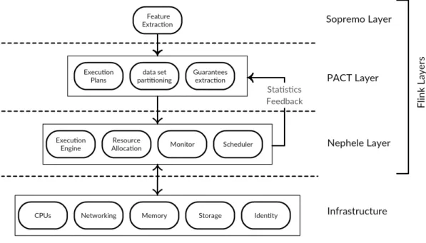
The Flink stack [25] consists of three layers: Sopremo, PACT, and Nephele, as depicted in Figure 3.1. These layers aim to translate the high-level programming language to a low-level one. Each layer represents a compilation step that tries to optimize the processing pipeline. Each layer comprises of a set of components that have certain responsibilities in the processing pipeline.
Figure 3.1: Flink stack
The Sopremo layer is responsible for operator implementations and information extraction from a job. It relies on an extensible query language and operator model called Sopremo [28]. This layer contains a compiler that enables extracting some properties from the submitted jobs at compile time. The extracted properties help in optimizing the submitted job in the following layers. A Sopremo program consists of logical operators in a DAG. Vertices represent tasks and edges represent the connections between the tasks. The Sopremo layer translates the submitted program to an operator plan. A PACT program [29] is the output of the Sopremo layer and the input to the PACT layer.
The PACT programming model is an extension to the MapReduce model calledPACTs [30]. The PACT layer divides the input data sets into subsets according to the degree of parallelism. PACTs are responsible for defining a set of guarantees to determine which subsets will be processed together. Processing subsets are based on first-order functions which are executed at run time. Similar to MapReduce model, the user-defined first-order functions are independent of the parallelism degree. In addition to the MapReduce features, PACTs can form complex DAGs.
The PACT layer contains a special cost-based optimizer. According to the guarantees defined by the PACTs, this layer defines different execution plans. The cost-based optimizer is responsible for choosing the most suitable plan for a job. In addition to the statistics which are collected by Flink’s resource manager, the optimizer decisions are influenced by the properties sent from the Sopremo layer. PACTs are the output of the PACT layer and the input to the Nephele layer.
The Nephele layer is the third layer in the Flink stack. It is the Flink’s parallel execution engine and resource manager. This layer receives data flow programs as DAGs and a certain execution strategy from the PACT layer that suggests the degree of parallelism for each task. Nephele executes jobs on a cluster of worker nodes. It manages the cluster’s infrastructure such as CPUs, networking, memory, and storage. This layer is responsible for resource allocation, job scheduling, execution monitoring, failure recovery, and collecting statistics about the execution time and the resource consumption. The gathered statistics are used in the PACT optimizer.
3.2.2
Streaming Engine
Flink has a streaming engine4 to process and analyze real-time data, which is able to read unbounded partitioned streams of data from external sources called DataS-treams. ADataStream aggregates data into time-based windows. It provides flexible windowing semantics where windows can be defined according to the number of records or a specific amount of time. DataStreams support high-level operators for processing data such as joins, grouping, filtering, and arithmetic operations.
When a stream processing job starts running on Flink, operators of DataStreams
become part of the execution graph in DAG. Each task is composed of a set of input channels, an operator state, a user-defined function (UDF), and a set of output channels. Flink pulls data from input channels and executes the UDF to generate the output. If the rate of injected data is higher than the data processing rate, a back pressure problem will appear5.
A data streaming pipeline consists of data sources, a stream processing job, and sinks to store results. In the normal case, the streaming job processes data at the same rate at which data is injected from the sources. If the stream processing job is not able to process data as fast as the injected data, the system could drop the additional data or buffer it somewhere. Data loss is not acceptable in m