Examining the potential of Floating Car Data for
Dynamic Traffic Management
Maarten Houbraken, Steven Logghe,
Pieter Audenaert, Didier Colle, Mario Pickavet
Abstract
Traditional traffic monitoring systems are mostly based on road side equipment measuring traffic conditions throughout the day. With more and more GPS enabled connected devices, Floating Car Data (FCD) has become an interesting source of traffic information, requiring only a frac-tion of the road side equipment infrastructure investment. While FCD is commonly used to derive historic travel times on individual roads and to evaluate other traffic data and algorithms, it could also be used in traffic management systems directly. However, as live systems only capture a small percentage of all traffic, its use in live operating systems needs to be examined. In this paper, we investigate the potential of FCD to be used as input data for live automated traffic management systems. The FCD in this study is collected by a live country-wide FCD system in the Netherlands covering 6-8% of all vehicles. The (anonymised) data is first compared to available road side measurements to show the current quality of FCD. It is then used in a dynamic speed management system and com-pared to the installed system on the studied highway. Results indicate the FCD setup can approximate the installed system, showing the feasibility of a live system.
1
Introduction
Digital connected devices have become widespread in the past decade. As people are travelling, these ‘smart’ devices can send and receive traffic information on the road. While this allows users to optimise their journey by avoiding traffic jams, it also improves the quality of the traffic information, as the data supplied by the users is fed back into the system and used to more accurately estimate traffic state. This source of data, termed Floating Car Data (FCD), presents an interesting opportunity in the field of traffic monitoring and analysis.
Traffic data generation has evolved significantly. Earliest field trials involv-ing probe vehicles were reported in the 90’s [1] with vehicles aggregatinvolv-ing and compactly transmitting data over low bandwidth connections and for predefined positions as no universal positioning (such as GPS) was available. These tech-nological limitations guided development in traffic monitoring to focus on road
side equipment (RSE), such as inductive loops which provide a detailed view on the traffic conditions at a specific location. A large body of research has since grown, focusing on using loop data for various applications such as travel time estimation [2, 3], travel time prediction [2] and vehicle re-identification [4]. While loop data system technology has matured, it remains prone to malfunc-tions (e.g. [5] reports>25% broken loop sensors in a Chinese city), requiring costly maintenance. Together with the localised nature of loop information, a need still exists for cost-effective, alternative systems covering larger areas.
Cellular communication networks can also be used to monitor travellers, using mobile phone call handover events to generate user position data [6, 7] but the complexity of user triangulation among cell towers hindered the break-through of the system.
With the introduction of GPS technology with better positioning informa-tion outperforming cellular triangulainforma-tion, a wide range of trial and producinforma-tion FCD systems were developed. One of the key characteristics among the different technical implementations is the sample frequency. As vehicles move throughout the network, they record and transmit their position periodically to the system for further processing and aggregation. The frequency of data transfer varies, depending on the available bandwidth of the underlying communication system and the energy consumption (in-car versus stand-alone battery-powered devices) ([8] provides a discussion on FCD transfer cost). High frequency sampling sys-tems with frequencies of one sample every 1-10 seconds allow very accurate vehicle tracking as the difference in successive positions is quite small. In low frequency systems, with sampling only every 30-60 seconds (or more), tracking is more complex. The exact vehicle path needs to be reconstructed/estimated as the vehicle can travel several kilometres between successive positions. This requires more complex map matching algorithms [9, 10, 11, 12].
While FCD is becoming more widespread, it still remains uncertain what penetration rate is necessary for the desired system performance. Depending on the intended application and data sample frequency, the required/advised fraction of all traffic varies. For travel time estimation, [13] uses a fleet of 1500 taxis in Stockholm to derive travel times for a 1.5 hour timeslot on a specific route with very low frequency sampling (data reports only every 2 minutes). The same Stockholm system is also used by [14] to estimate route travel time distributions on 27 selected routes. Neural networks are applied in [15] to link travel time estimation with FCD although most results are based on simulated data. For a cellular-based FCD system, [6] reports results for travel times covering 1-3% of all traffic on average while [16] states success with 2.4% of all private cars in Rome. Similarly, [17] suggests 2.4 and 10% for highways and arterial roads respectively and [18] hints at 2-3% for cell phone based systems.
For incident detection, most installed systems use pure infrastructure based data collection (e.g. California algorithm [19] and McMaster algorithm [20]). Using vehicle-to-roadside communication, [21] monitors cars passing fixed mea-surement locations to estimate vehicle headways and lane switches to detect incidents. Looking at speed changes, the UCB algorithm [22] detects incidents from an FCD dataset with an estimated 0.1% coverage. In [23], the UCB
algo-rithm is compared to a CUSUM algoalgo-rithm which uses increased travel time in moving time windows. Using a modified CUSUM algorithm, [24] monitors flood-ing events in Beijflood-ing. Startflood-ing from 40000 taxis providflood-ing data every minute, they detect the specific FCD characteristics when roads are flooded and re-port these events. Relying solely on FCD for incident detection, [25] advises 1% while [26] reports 1.5%. In [27], the operational Dutch automated incident detection (AID) system (also used in this paper) is studied on 1.6 km British motorway with interpolated loop data. The Dutch AID is a queue tail warn-ing system coupled to an overhead variable message sign (VMS) system with variable speed limits (VSL) being displayed. The study found 1% FCD pene-tration rate required for similar performance compared to loop based systems. While reliability requirements differ among the applications and various tech-nical specifications e.g. frequency, latency and data aggregation impact the required penetration rate significantly, overall, the reported percentages are in the range of 1 to 10%, indicating the order of magnitude required.
One of the main directions in current research is how to combine FCD with RSE to achievedata fusion. Both FCD and loop data are used simultaneously in [28] to estimate the fundamental diagram. Similarly, [29] fuses camera data with FCD while [30] fuses loop data with FCD to estimate traffic conditions.
This paper focuses on the potential of FCD for dynamic traffic management, more specifically variable speed limits to a.o. homogenise traffic speeds or pre-vent end-of-queue collisions (see [31]). Most current day traffic management systems rely on RSE because these provide a more complete and detailed view on the traffic conditions (as they monitor all traffic). However, for large scale network monitoring, FCD is more interesting as it does not require additional measuring infrastructure, compared to RSE needing to be installed on all roads of interest. FCD does require sufficient probe vehicles, with the penetration rates studies mentioned above. However, most of these studies are based on simulated FCD and/or small FCD systems, thereby limiting the significance of the results. For example, [27] studies the application of FCD but uses in-terpolated loop data as FCD and uses a theoretical evaluation benchmark to determine FCD suitability. In this paper, we bridge this gap by using real FCD collected by an operational country-wide FCD platform and comparing it to the live captured output of the installed system. The rest of this paper is structured as follows. Before the main focus of this study is presented, Section 2 first de-tails the existing loop installation and traffic management algorithm on Dutch highways. Section 3 is dedicated to examining the potential of FCD for dynamic traffic management by proposing an FCD based speed advice algorithm. Sec-tion 4 proposes the comparison methodology used to compare the loop to the FCD VSL algorithm. Section 5 shows the global results of the algorithm.
2
Existing system & infrastructure
While in this study, we focus on the FCD potential, we first present the currently operational Automated Incident Detection (AID) system in our study area,
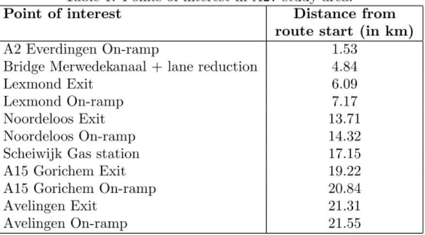
shown in Fig. 1 and annotated in Table 1. The Dutch highway loop AID system contains a queue tail warning system to improve traffic conditions and road safety. This system focuses on detecting congestion and other incidents and warns upstream traffic by using dynamic overhead signs. Once congestion is detected, drivers are alerted to reduce their speed and avoid rear-end collisions.
Table 1: Points of interest in A27 study area.
Point of interest Distance from
route start (in km) A2 Everdingen On-ramp 1.53
Bridge Merwedekanaal + lane reduction 4.84
Lexmond Exit 6.09
Lexmond On-ramp 7.17
Noordeloos Exit 13.71
Noordeloos On-ramp 14.32
Scheiwijk Gas station 17.15
A15 Gorichem Exit 19.22
A15 Gorichem On-ramp 20.84
Avelingen Exit 21.31
Avelingen On-ramp 21.55
The system consists of overhead signs installed above the highway, with each dynamic road sign coupled to a dual inductive loop. Each sign keeps a running averagevcurof the individual vehicle speeds registered by the loop sensor. When
a car passes the sensor with a speedvslower than vcur, the current average is
changed to (1−αdec)·vcur+αdec·vs. If vs ¿ vcur, the update is done with
a different weighting factor αacc to allow different switching behaviour when
traffic is speeding up or slowing down.
Parametersαaccandαdecallow to tune the sensitivity of the average to faster
and lower samples respectively, with 0≤αacc, αdec ≤1. The weighted speeds
vcur are monitored to detect congestion events and other incidents. When an
individual vcur drops below a predefined lower threshold von e.g. 35 km/h,
the controller switches on the overhead sign. When traffic improves and vcur
becomes larger than the upper thresholdvof f e.g. 50 km/h, the sign is switched
off and will showBLK (=blank). These thresholds can be set differently (with
von ≤vof f), creating hysteresis to avoid excessive switching of the road sign.
The values forvonandvof f were set by the Dutch road side operators according
to their desired sign switching.
While each controller determines its sign based on its ownvcur, the individual
controllers are also linked to allow overall consistent signage. Controllers at the same location but monitoring different lanes communicate to avoid inconsistent speed advices e.g. the leftmost lane getting a lower speed advice than the right-most lane. While the signs on the individual lanes can differ, this only occurs when road operators input manual overrides from the regional traffic manage-ment central. Controllers also take into account the first downstream detector
Figure 1: Overview of A27 study area. The monitored route (in red) runs from Vianen (top right) southbound to Gorinchem (bottom left). The points of interest of Table 1 are marked by the blue markers.
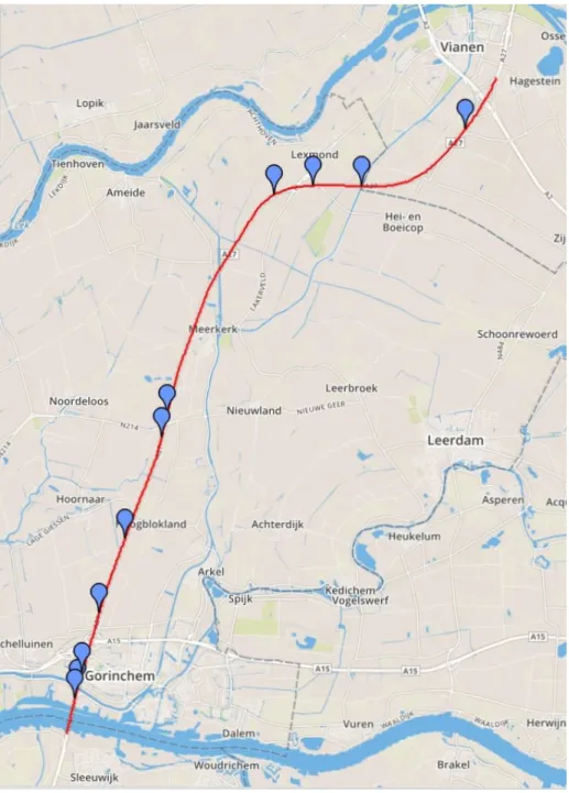
Figure 2: Spatio-temporal plot of the loop VSL on the A27 highway on Thurs-day 14 January 2016, from 3 pm to 9 pm. The installed overhead signs shows 50 km/h (orange) in the detected traffic jam itself, 70 km/h (yellow) just up-stream of the congestion andBLK (white) outside of the congestion. The black vertical lines denote the positions of interest from Table 1.
(typically within 500 m) to better capture backward propagating congestion waves. When a speed sign is activated by its controller, the first upstream con-troller (within 500 m) also activates its road sign, allowing drivers to be alerted before the congestion wave reaches the next controller location. The second upstream controller (within 1000 m) is also alerted to activate an additional (less strict) speed advice, to slow down traffic more gradually. Note that the distances given are typical values, as the distance between loops can vary.
This system thus converts individual vehicle samples to incident reports and dynamic speed advice along the highway. As an individual sign at a specific location is valid on the route until the next downstream sign, the combined signage provides dynamic speed advices for the entire route with a granularity depending on the installed loop hardware. For the A27 route in our study, Fig. 2 shows the individual road signs throughout the day. The black vertical lines, denoting the positions of interest from Table 1, are plotted to explain some structural properties of the road e.g. the 3-to-2 lane reduction bottleneck at km 4.84.
3
FCD System
The aim of this paper is to show the potential of FCD for dynamic traffic management. In this section, we first elaborate on the FCD properties of the underlying FCD system before presenting the FCD algorithm.
3.1
FCD data
The main difference between FCD and loop data is the distributed nature of ve-hicle tracking. FCD consists of individual probe veve-hicle measurement samples, each denoted with a timestamp, an anonymised identifier, a set of coordinates, a speed estimatevsand a vehicle heading. As mentioned in Section 1, the FCD
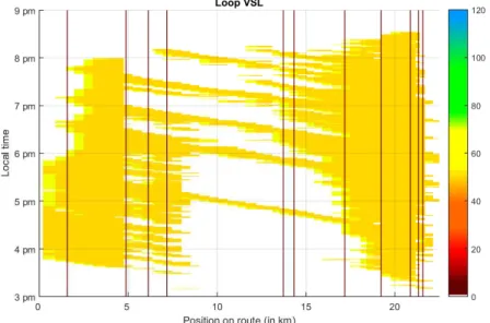
sampling rate varies significantly and impacts the additional processing required for converting the distributed data. For this study, we use high frequency FCD, with probe vehicles generating data samples every second. This allows to min-imise the data capturing delay the algorithm (see next section) experiences. The samples were matched to an underlying representation of the road network consisting of road segments of 50 m using their coordinates and heading. The system used to generate data in this study operates in the Netherlands, combin-ing positioncombin-ing data obtained from transport companies as well as from mobile apps. While the system works for the entire country, the area of study is limited to the A27 (see Fig. 1). The general system setup consists of instrumented ve-hicles that sample their own position and speed and relay this information to a central server for processing (to aggregate to average travel times). Fig. 3 shows the FCD consisting of individual vehicle trajectories matched to the underlying road.
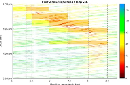
Compared to the loop data, the FCD provides data for road segments be-tween loop locations, revealing the traffic conditions and congestion evolution along the route more clearly. This is illustrated in Fig. 4, showing the formation of a backward propagating traffic jam around km 8 at 4 pm. Traffic congestion develops at the loop around 3:56 pm. It travels a little further along the route before turning into a backwards propagating traffic jam. The loop VSL does not activate until the congestion reaches the loops at km 8. Also note the loop VSL switches off several times (e.g. around 4:05 pm) as the small congestion wave travels backwards. Thevcur of the detector at km 7.5 is not low enough
to trigger the AID, while thevcur at km 8 is already higher than thevof f.
3.2
FCD VSL
Using the high frequency FCD described above, a VSL system similar to the installed loop AID/VSL system can be developed. While the loop system has a set of fixed portal locations roughly every 500 m, the matched FCD is avail-able on each 50 m segment of the underlying map. On each such segment, a virtual road sign controller is defined, working on the FCD for that segment. As with the loop system, the virtual FCD road sign controller keeps a weighted sum of the vehicle samples on the segment with updates for every new sample
Figure 3: Individual FCD vehicle trajectories A27 highway on Thursday 14 January 2016, from 3 pm to 9 pm. Vehicles drive from the left to right, with their speeds being colour-coded in the figure. When multiple vehicles are on the same segments, their average speed is shown.
Figure 4: FCD vehicle trajectories and loop variable speed limit signs, detailed view for 15 December 2015. Loop portal locations are indicated by the vertical dashed lines. FCD is plotted as in Fig. 3, loop VSL are plotted as an overlay using the same colour code as in Fig. 2.
Figure 5: FCD VSL result on the A27 highway on Thursday 14 January 2016, from 3 pm to 9 pm. The FCD algorithm, using the data shown in Fig. 3, generates speed advice of 50 and 70 km/h which are colour-coded as orange and yellow, respectively.
according to the procedure in Section 2. For a route of 22.5 km, this results in 450 segments with associated virtual controllers keeping a weighted sum. Whenever one of these values goes below the predefined threshold (similar to the loop system), the segment is considered to be congested. As with the loops, this triggers an alert for the current segment. However, to mimic the inter-connected upstream/downstream loop controllers, the congested status of one virtual detector also triggers speed advice on all segments 500 m upstream and downstream, as well as a less strict advice for segments between 500 and 1000 m upstream. The resulting FCD VSL is illustrated in Fig. 5. While the loop system works with blocks of 500 m, the FCD VSL has a higher granularity, depending on the road map segment size. This higher granularity allows for better traffic jam monitoring.
4
Evaluation methodology
To evaluate the quality of the FCD, we focus on the experimental data from the underlying FCD system and the installed loop AID. With the detailed loop logs and the high frequency FCD with a 6-8% penetration rate, it is possible to focus on the experimental data instead of using micro-simulations for which the results would be tightly coupled to the simulation parameters. We compare the result
of the loop VSL to that of the FCD VSL, focusing on the signage results rather than on the data itself. This allows to fairly compare both systems, as they both provide speed advice for the entire space-time window of the study area. This is the biggest motivation for focusing on the signage results, as purely comparing loop data to FCD is infeasible, with both sources fundamentally differing in terms of data granularity, covered area and data frequency. Furthermore, data quality also depends on the intended application scenario. With both systems providing a full response for the spatio-temporal study area, the loop system is used as a reference for the FCD algorithm.
4.1
State modelling
The following analysis was done on the output of both VSL systems. However, comparing the FCD VSL to the loop VSL also needs careful modelling. A first, straightforward evaluation could be to compare the individual systems output for each timeslot and position in the considered space-time window. While this is simple, it fails at capturing the underlying traffic conditions and comparing both sources. If one source proposes “50” while the other gives no indication, it is unclear what the actual best sign should be. Similarly, if one system would decide on a “70” while the other is now at “50” after already displaying “70” for a few minutes, what penalty should be applied? To clearly differentiate between both systems, the temporal switching/evolution of the signs needs to be accounted for.
The first step in the following analysis consists of modelling the individual sources in temporal states. With the system being discretised in individual space-timeslots, each of those slots is classified according to its current, past and future sign. As the system under study allows for 3 different sign outputs (“BLK” in free flow, “50” and “70” in congestion), the classification yields 33 = 27 possible states. The state for each space-timeslot is determined by looking at the temporal switching at each position. While the current sign is directly available as the output of the system at that position, the past and future signs need further processing. The future sign for the current space-timeslot is determined by taking the (temporally) next sign at that location. If the system currently proposes “70” at the considered location, the future sign is the sign it will switch to in the future. Note however, that this look-ahead is limited to the immediate future, with a window of 1 minute. If no sign switch would occur, the current sign is considered to persist and taken as the future sign as well. A similar definition is used for the past sign, but looking back in time at that location. Given these definitions, a sign that is currently showing “50”, but was showing “70” 30 seconds ago and will show nothing in 40 seconds, will be classified as being in the (70,50, BLK) state.
4.2
State-based comparison
Using this VSL system classification, the 2 systems are more accurately com-pared. Each space-timeslot of the considered window is classified in one of the
Figure 6: Category classification A27 highway on Thursday 14 January 2016, from 3 pm to 9 pm.
N ×N possible (stateLoop, stateF CD) combinations. Here N = 33 = 27, yielding 27×27 = 729 combinations. To allow a more tangible analysis on the VSL system level, the states were first grouped according to the situation they correspond to. These categories are summarised in Table 2.
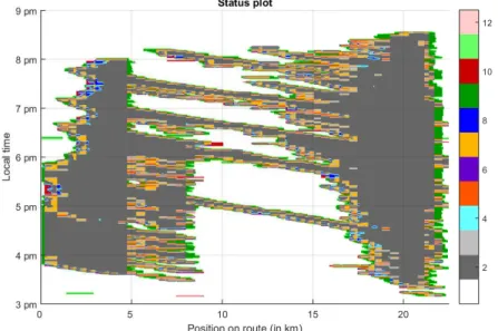
This classification gives an indication of the similarity of 2 VSL systems, as well as the specific conservative/relaxed differences between them. A VSL system is termed to be more conservative than the other if it shows a lower speed advice or if the advices are equal but it is going to show a lower speed advice e.g. (BLK,50,50) is more conservative than (BLK,50,70). An example of the classification is shown in Fig. 6. Each space-timeslot of 50 m and 1 s is colour-coded according to the categories of Table 2. With category 2 being prevalent during congestion, the main differences are on the edges of the traffic jam, due to differences in switching behaviour between both algorithms.
To obtain overall comparison metrics, the relative fractions of each category are calculated. This is shown in Table 2 for the study in this paper. The
Correspondence Score weight is explained in the following section.
4.3
FCD VSL calibration
The proposed VSL system analysis can now be used as a tool in the high level system comparison and to test the effect of individual VSL system parameter changes. Changing specific parameters in the FCD algorithm (see Section 3.2), will result in some of the space-timeslots ending up in different categories,
shift-T able 2: Categorisation of VSL syste m com binations. Note that “ − ” is used to compactly denote “BLK” while “?” is a placeholder for “BLK”, 50 and 70. Category Description Corresp ondence co de Score w eigh t 1 Both systems are idle (e.g. lo w traffic), corresp onding to state ( − , − , − )-( − , − , − ) 1 2 Both systems are in the same state 1 3 Both systems sho w the same sign but F CD VS L is in a more conserv ativ e/restricted state .5 4 Both systems sho w the same sign but F CD VS L is in a more relaxed state 0 5 Lo op VSL sho ws nothing (but has sho wn or will sho w), F CD VSL is already sho wing .5 6 F CD VSL sho ws nothing (but has sho wn or will sho w), Lo op VSL is already sho wing -1 7 Both sho w something but F CD VSL is more restrictiv e .5 8 Both sho w something but F CD VSL is more relaxed -.5 9 Lo op VSL is idle ( − , − , − ), F CD VSL sho ws something (? , ? 6 = − , ?) 0 10 F CD VSL is idle ( − , − , − ), Lo op VSL sho ws something (? , ? 6 = − , ?) -2 11 Lo op VSL is idle ( − , − , − ), F CD VSL sho ws “BLK” but is a w are of problems (? , − , ?) 6 = ( − , − , − ) 0 12 F CD VSL is idle ( − , − , − ), Lo op VSL sho ws “BLK” but is a w are of problems (? , − , ?) 6 = ( − , − , − ) -.5
ing the metrics. More interestingly, the analysis metrics can be used in an optimisation study of the FCD VSL parameters.
The FCD parameters were calibrated to best approximate the switching behaviour of the existing, country-wide implemented AID system. The 12 cate-gories from above were weighted to produce a single metric, theCorrespondence Score(CS). The CS aims at estimating the overall correspondence of the FCD AID system to the loop AID system. Each category received a weight factor (see Table 2) based on how well the category is desirable to mimic the loop sys-tem. The higher the weight, the more desirable the category is. These weights are currently chosen to obtain a conservative FCD VSL system, warning more proactively, in order to capture all situations in which the loop system also activates. Other weights can be specified according to user preferences.
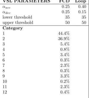
Starting from the FCD of 14 January 2016, the FCD AID results were calcu-lated along with the CS for different parameter combinations. In the optimisa-tion procedure, the sample weighting factorsαacc andαdec were varied from .1
to .6 in increments of .05. The upper threshold was varied from 40 to 55 km/h while the lower threshold was varied from 25 to 40 km/h, both in increments of 5 km/h. The influence range of the virtual detectors (500 m) was not varied as these were considered to correspond well to the current AID guidelines for loop placement on Dutch highways. Maximal correspondence was obtained for the presented use case for the parameters shown in Table 3. Comparing the
Table 3: Optimal FCD parameters for conservative loop AID approximation for A27 highway on Thursday 14 January 2016, from 3 pm to 9 pm.
VSL PARAMETERS FCD Loop αacc 0.25 0.40 αdec 0.25 0.15 lower threshold 35 35 upper threshold 50 50 Category 1 44.4% 2 36.9% 3 5.4% 4 0.8% 5 3.4% 6 0.3% 7 2.3% 8 0.3% 9 3.3% 10 0.2% 11 2.3% 12 0.4% Correspondence Score 0.8575
values of the FCD VSL algorithm to those of the loop VSL (as set by the Dutch road side operator), the upper and lower thresholds are the same. The αacc
is lower whileαdec is somewhat higher, indicating higher speeds are taken into
account less while lower speeds more. This makes the average calculated by the virtual loop detectors react quicker to lower speeds, which results in going below the lower threshold quicker. It should however again be noted that opti-mising for correspondence aims at approximating the loop system. Due to its inherent technological properties, the loop system has its own advantages and limitations (e.g. spatial resolution, limited look-ahead), as well as the FCD sys-tem. Optimising for correspondence could lead to unwanted effect as the FCD system would overfit and try to optimise out some of its inherent advantages compared to the loop system. It does however show the potential of current FCD to generate VSL signage.
5
Evaluation
With the described evaluation above, the calibrated FCD VSL is compared to the Loop VSL for an extended period of time. Table 4 shows the comparison for the weekdays between January 11 and January 22, 2016. Compared to the loop data, the FCD coverage varies between 6-8% of all traffic. For each day, the state categorisation from above was done, resulting in the relative percentages for each category. On top of the correspondence score (CS), the table also aggregates the different categories to overall percentages to show the similarity and conservative nature of both systems. TheIdlestate classification corresponds to the percentage that both systems were idle (category 1) while the
Identicalstate denotes the portion that both systems were in the same 3-valued state from above (category 2). The Conservative classification represents the sum of the categories in which the FCD system was more cautious than the loop system (categories 3, 5, 7, 9 & 11). Relaxed denotes the opposite, with the loop system being more cautious (categories 4, 6, 8, 10 & 12). When the loop VSL is taken as the reference, the relaxed portion gives an indication of missed signs. Note however that the loop system itself has some disadvantages, as shown in Section 3.1.
Additionally, the table also sums the different categories but only taking into account the actual displayed sign for the drivers. This results in the Iden-tical (categories 1, 2, 3, 4, 11 & 12), Conservative (categories 5, 7 & 9) and
Relaxed (categories 6, 8 & 10) sign entries. These numbers give more insight into the perceived difference by an observer not taking into account temporal sign switching.
In the 2 weeks shown here, the 12th and 14th of January had severe con-gestion while Friday 15 January hardly had any concon-gestion. Excluding these days, the average fraction idle states is 71.1%, with 15.9% identical, 11.7% more conservative and 1.4% more relaxed state classification. For the sign classifica-tion, the averaging of the 7 days yields 93.1% identical, 6.2% more conservative and 0.6% more relaxed signage. On the congested days, the VSL systems were
T able 4: Comparison F CD VSL to lo op VSL for A27 high w a y for w eekda ys from Monda y 11 Jan uary to F rida y 22 Jan uary 2016, b et w een 3 pm and 9 pm. Date MON 11 Jan TU E S 12 Jan WED 13 Jan THU 14 Jan FRI 15 Jan ST A TE Idle 72.7% 46.1% 70.0% 44.4% 95.0% Iden tical 14 .6% 36.0% 16.9% 36.9% 1.9% Conserv ativ e 11.1% 15. 7% 11.8% 16.7% 2.9% Relaxed 1.6% 2.3% 1.3% 2.0% 0.2% SIGN Iden tical 93 .1% 90.7% 93.4% 90.1% 98.2% Conserv ativ e 6.1% 8. 3% 6.1% 9.0% 1.7% Relaxed 0.8% 1.0% 0.6% 0.9% 0.1% CS 0.8965 0.8586 0.8973 0.8575 0.9732 Date MON 18 Jan TU E S 19 Jan WED 20 Jan THU 21 Jan FRI 22 Jan ST A TE Idle 77.9% 70.9% 67.9% 67.7% 70.4% Iden tical 13 .1% 16.0% 18.1% 17.3% 15.1% Conserv ativ e 8.2% 11. 7% 12.5% 13.5% 13.2% Relaxed 0.9% 1.4% 1.4% 1.4% 1.4% SIGN Iden tical 94 .7% 93.2% 93.0% 92.1% 92.5% Conserv ativ e 4.9% 6. 0% 6.3% 7.3% 6.9% Relaxed 0.4% 0.8% 0.8% 0.6% 0.6% CS 0.9290 0.8975 0.8874 0.8884 0.8896
active for more than half of the study window as indicated by the idle state percentages 46% and 44%. Compared to normal inactivity of 71.3%, the in-crease in the relaxed signs is limited as they only inin-creased from 0.6% (average normal days) to 0.9% (average for the 2 congested days). This indicates that the increase in the relaxed classification is caused by the increased activity of the VSL systems. Looking at the non-congested Friday 15 January, the FCD VSL is only more relaxed in 0.1% of the window. Overall, the low fraction of the relaxed classification is due to the conservative calibration of the FCD sys-tem. While the numbers for the relaxed classification should not be minimised, it does indicate that the calibrated FCD VSL (using only 1 day) approximates the loop VSL and is a suitable alternative.
5.1
Real time potential analysis
In the analysis above, all data was considered to be available instantaneously to the AID systems. In real applications, some delay will be present, mostly attributable to communication overhead and FCD transmission schemes. While the loop systems are operational, proving their feasibility, the tolerable latency for FCD is yet unknown. This section aims at investigating the effects of latency on the FCD VSL system.
To study the effect of latency, artificial delay is introduced in the FCD VSL algorithm. FCD samples are simulated to have a fixed communication overhead. While this latency in real life would be more random, it is sufficient here to show the performance impact. The FCD parameters in both cases are set to the optimal values from before. Delay was added in steps of 5 seconds. Fig. 7 shows the Relative Correspondence Score (RCS) for the A27. The RCS is the ratio of the CS for each specific latency to the maximum CS (when no FCD delay is present). Negative delay values (e.g. -60 s) correspond to situations where the loop data (used for the loop AID) would have delay before being accounted for in the overhead signs, as the CS is relative between both VSL systems. Interestingly, the conservative calibration of the FCD parameters results in a better tolerance for positive FCD delay, with a graceful degradation of the RCS of 0.0055% per second of added latency, than for negative FCD delay, with degradation of 0.0065%. The conservative nature of the FCD calibration makes it warn earlier, lessening the impact of the FCD delay.
Note that the analysis here was done without optimising any FCD system parameter. In live systems, these parameters could be adjusted (based on a preliminary estimate of the experienced latency) to account for the expected latency. By tweaking the αdec of the FCD VSL, it could be more proactive
in alerting for congestion. Similarly, the influence range could be enlarged, to account for backwards congestion propagation. Furthermore, more specific approaches could be used in the FCD algorithm e.g. including the sample age (to account for variable latency) or taking into account downstream samples in the estimation for the current position. Specialised provisions for latency are beyond the scope of this paper as the focus here was to show the potential of FCD in terms of traffic estimation and VSL application.
S2
S%
4
5a
5s
5o
5−
lee
SS2S4
lee
ce
e
ce
lee
6
Discussion
While the results above indicate the potential of FCD, some important remarks need to be made. Firstly, the algorithm was designed/calibrated to mimic the existing loop system, as this was the only available reference. While loop sys-tems are widely used, they have known disadvantages e.g. localised view and prone to sensor errors. Aside from costly manual benchmarks and model-bound simulation results, no reference output exists. For this study, the operational system, having proven its value in the field, was considered a good target for FCD testing. Other VSL logs could however easily be integrated in the calibra-tion/evaluation. This would also allow to use some FCD properties (e.g. time between samples or total number of samples) which were not included in the algorithm design to stick close to the reference. Fully utilising valuable FCD properties is left for future work.
Another point of interest is the used FCD. In our study, high frequency FCD covering 6-8% of traffic was available. Compared to the existing literature (see introduction), this is a lot of data. The performance of the FCD algorithm with less data would decline. However, considering advances in vehicle commu-nication and connectivity, cellular coverage and emerging tolling policies, data availability will only increase. By properly integrating our modern infrastruc-ture (taking privacy into account), the penetration rates will improve, allowing for even better results. While results of our algorithm on smaller datasets would be interesting to determine the absolute required FCD penetration rate, the imperfect benchmark, varying desired performance and omitted algorithm optimisations render optimal parameters not sensible. Extensive optimisation studies are left for future work.
7
Conclusion
In this paper, we focused on the potential for Floating Car Data (FCD) to be used in dynamic traffic management systems. An FCD variable speed limiting (VSL) algorithm was designed similar to an existing loop VSL and evaluated by a state based classification method. The FCD VSL was conservatively calibrated and compared to an existing loop VSL benchmark during afternoon rush hour for 2 work weeks. The FCD VSL followed loop signage throughout the study period, only not warning 0.6% of the time window on normal days and 0.9% on congested days. This live setup shows that current FCD system technology has acceptable latency and sufficient penetration rate to allow live VSL. With lower system costs, wider area coverage and ever-increasing vehicle connectivity, FCD presents a valuable alternative for loop data in dynamic traffic management systems.
Acknowledgment
Maarten Houbraken was a PhD fellow of the Research Foundation - Flanders (FWO-Vlaanderen). The authors would further like to thank the Dutch road side operator RWS for providing the data.
References
[1] M. Westerman, R. Litjens, J.-P. Linnartz. “Integration Of Probe Vehicle And Induction Loop Data: Estimation Of Travel Times And Automatic Incident Detection”, Technical report, Institute of Transportation Studies, University of California, Berkeley, (1996).
[2] J. Kwon, B. Coifman, P. Bickel. “Day-to-Day Travel Time Trends and Travel Time Prediction from Loop Detector Data”, Transportation Re-search Record,(1717), pp. 120–129, (2000).
[3] B. Coifman. “Estimating travel times and vehicle trajectories on freeways using dual loop detectors”, Transportation Research Part A: Policy and Practice,36(4), pp. 351–364, (2002).
[4] B. Coifman. “Vehicle Re-Identification and Travel Time Measurement in Real-Time on Freeways Using Existing Loop Detector Infrastructure”,
Transportation Research Record: Journal of the Transportation Research Board,1643(July), pp. 181–191, (jan 1998).
[5] J. Li, H. van Zuylen, G. Wei. “Diagnosing and Interpolating Loop Detector Data Errors with Probe Vehicle Data”, Transportation Research Record: Journal of the Transportation Research Board,2423, pp. 61–67, (2014). [6] H. Bar-Gera. “Evaluation of a cellular phone-based system for
measure-ments of traffic speeds and travel times: A case study from Israel”, Trans-portation Research Part C: Emerging Technologies, 15(6), pp. 380–391, (dec 2007).
[7] D. Gundlegard, J. Karlsson. “Handover location accuracy for travel time estimation in GSM and UMTS”,IET Intelligent Transport Systems,3(1), p. 87, (2009).
[8] S. Ancona, R. Stanica, M. Fiore. “Performance boundaries of massive Floating Car Data offloading”, 2014 11th Annual Conference on Wireless On-demand Network Systems and Services (WONS), pp. 89–96, (IEEE, 2014).
[9] M. A. Quddus, W. Y. Ochieng, R. B. Noland. “Current map-matching al-gorithms for transport applications: State-of-the art and future research di-rections”,Transportation Research Part C: Emerging Technologies,15(5), pp. 312–328, (oct 2007).
[10] F. Chen, M. Shen, Y. Tang. “Local Path Searching Based Map Match-ing Algorithm for FloatMatch-ing Car Data”, Procedia Environmental Sciences, 10(PART A), pp. 576–582, (2011).
[11] T. Miwa, D. Kiuchi, T. Yamamoto, T. Morikawa. “Development of map matching algorithm for low frequency probe data”,Transportation Research Part C: Emerging Technologies,22, pp. 132–145, (2012).
[12] B. Y. Chen, H. Yuan, Q. Li, W. H. Lam, S.-L. Shaw, K. Yan. “Map-matching algorithm for large-scale low-frequency floating car data”, Inter-national Journal of Geographical Information Science, 28(1), pp. 22–38, (2014).
[13] E. Jenelius, H. N. Koutsopoulos. “Travel time estimation for urban road networks using low frequency probe vehicle data”,Transportation Research Part B: Methodological,53, pp. 64–81, (jul 2013).
[14] M. Rahmani, E. Jenelius, H. N. Koutsopoulos. “Non-parametric estimation of route travel time distributions from low-frequency floating car data”,
Transportation Research Part C: Emerging Technologies,58, pp. 343–362, (sep 2015).
[15] F. Zheng, H. Van Zuylen. “Urban link travel time estimation based on sparse probe vehicle data”, Transportation Research Part C: Emerging Technologies,31(111), pp. 145–157, (2013).
[16] C. De Fabritiis, R. Ragona, G. Valenti. “Traffic estimation and predic-tion based on real time floating car data”,IEEE Conference on Intelligent Transportation Systems, Proceedings, ITSC, (NOVEMBER 2008), pp. 197–203, (2008).
[17] S. Breitenberger, B. Gr¨uber, M. Neuherz, R. Kates. “Traffic information potential and necessary penetration rates”, Traffic Engineering and Con-trol,45(11), pp. 396–401, (2004).
[18] J. C. Herrera, D. B. Work, R. Herring, X. J. Ban, Q. Jacobson, A. M. Bayen. “Evaluation of traffic data obtained via GPS-enabled mobile phones: The Mobile Century field experiment”, Transportation Research Part C: Emerging Technologies,18(4), pp. 568–583, (aug 2010).
[19] M. Levin, G. M. Krause. “Incident detection: A Bayesian Approach”,
Transportation Research Record, (682), pp. 52–58, (1978).
[20] A. I. Gall, F. L. Hall. “Distinguishing Between Incident Congestion and Re-current Congestion: A Proposed Logic”, Transportation Research Record, (1232), pp. 1–8, (1989).
[21] E. Parkany, D. Bernstein, E. Parkany. “Design of Incident Detection Al-gorithms Using Vehicle-to-Roadside Communication Sensors”, Transporta-tion Research Record 1494,67, pp. 67–74, (1995).
[22] K. Petty, A. Skabardonis, P. Varaiya. “Incident Detection with Probe Ve-hicles: Performance, Infrastructure Requirements, and Feasibility”, IFAC Proceedings Volumes,30(8), pp. 125–130, (jun 1997).
[23] L. Yu, L. Yu, Y. Qi, J. Wang, H. Wen. “Traffic Incident Detection Al-gorithm for Urban Expressways Based on Probe Vehicle Data”, Journal of Transportation Systems Engineering and Information Technology,8(4), pp. 36–41, (2008).
[24] L. Yu, Y. Gao, L. Yu, G. Song, F. Zhang, J. Liu. “Floating car data-based method for detecting flooding incident under grade separation bridges in Beijing”,IET Intelligent Transport Systems,9(8), pp. 817–823, (oct 2015). [25] W. Vandenberghe, E. Vanhauwaert, S. Verbrugge, I. Moerman, P. De-meester. “Feasibility of expanding traffic monitoring systems with floating car data technology”, IET Intelligent Transport Systems, 6(4), pp. 347– 354, (dec 2012).
[26] B. Kerner, C. Demir, R. Herrtwich, S. Klenov, H. Rehborn, M. Aleksi, A. Haug. “Traffic state detection with floating car data in road networks”,
Proceedings. 2005 IEEE Intelligent Transportation Systems, 2005., pp. 700– 705, (IEEE, 2005).
[27] G. Klunder, H. Taale, S. Hoogendoorn. “The Impact of Loop Detector Distance and Floating Car Data Penetration Rate on Queue Tail Warning”,
3rd International Conference on Models and Technologies for Intelligent Transport Systems, (2013).
[28] L. Amb¨uhl, M. Menendez. “Data fusion algorithm for macroscopic funda-mental diagram estimation”, Transportation Research Part C: Emerging Technologies,71, pp. 184–197, (oct 2016).
[29] M. Rahmani, E. Jenelius, H. N. Koutsopoulos. “Floating Car and Camera Data Fusion for Non-Parametric Route Travel Time Estimation”, 2014 IEEE 17th International Conference on Intelligent Transportation Systems (ITSC), pp. 1286–1291, (2014).
[30] M. Houbraken, P. Audenaert, D. Colle, M. Pickavet, K. Scheerlinck, I. Yperman, S. Logghe. “Real-time traffic monitoring by fusing floating car data with stationary detector data”,2015 International Conference on Models and Technologies for Intelligent Transportation Systems, MT-ITS 2015, (2015).
[31] C.-s. Chou, A. P. Nichols. “Deriving a surrogate safety measure for free-way incidents based on predicted end-of-queue properties”,IET Intelligent Transport Systems,9(1), pp. 22–29, (feb 2015).