D. S. Lee†‡*, L. F. Gonzalez‡, J. Périaux‡and K. Srinivas†
†
School of Aerospace Mechanical Mechatronic Engineering (AMME), University of Sydney, NSW 2006, Australia. [email protected], [email protected]
‡
School of Engineering System, Queensland University of Technology, Brisbane Australia.
CIMNE/UPC, Barcelona, Spain and INRIA Sophia OPALE Project Associate.
Abstract: One of the new challenges in aeronautics is combining and accounting for multiple disciplines while considering uncertainties or variability in the design parameters or operating conditions. This paper describes a methodology for robust multidisciplinary design optimisation when there is uncertainty in the operating conditions. The methodology which is based on canonical evolution algorithms is enhanced by its coupling with an uncertainty analysis technique. The paper illus-trates the use of this methodology on two practical test cases related to Unmanned Aerial Systems (UAS). These are the ideal candidates due to the multi-physics in-volved and variability of missions to be performed. Results obtained from the op-timisation show that the method is effective to find useful Pareto non-dominated solutions and the use of robust design techniques.
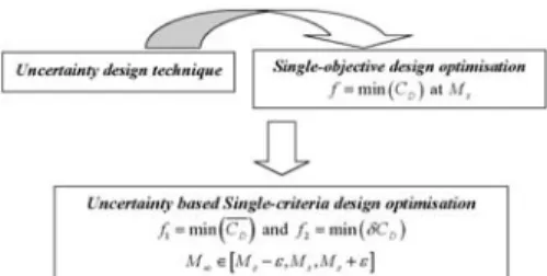
4.1.1 Introduction
Most of Multi-Objective (MO) and Multidisciplinary Design Optimisation (MDO) problems in aerospace engineering frequently deal with intuitive nature problems [1-3]. One cannot ignore the fact that MO and MDO in aerospace engineering fre-quently deal with situations where the design input parameters and flight/flow conditions have some amount of uncertainty. When the optimisation is carried out for fixed values of the design variables and parameters however, converged opti-mised solution results in good performance at design condition but poor drag or lift to drag ratio at slightly off-design conditions. The challenge in aeronautics is still to develop a robust design that accounts for uncertainty in the design or
oper-ating conditions of the engineering system or aircraft. In this work we attempt to remedy this issue and prevent the fluctuation of performance by using a robust de-sign technique [5, 6].
This paper introduces uncertainty based robust design coupled with evolutionary algorithms and analysis tools for aerodynamics, electro-magnetics to maximise the survivability of Unmanned (Combat) Aerial Vehicles (UAV/UCAV) at a set of variable flight conditions and frequencies that affect the Radar Cross Section (RCS). The paper describes the methodology and its numerical implementation for Uncertainty based Multidisciplinary Design Optimisation (U-MDO). The method-ology couples a CFD and RCS analysis software, an advanced evolutionary opti-miser (HAPMOEA) [7] and the concept of robust/uncertainty strategy in the de-sign, to produce a set of optimal –stable designs.
The rest of paper is organised as follows; Section 4.1.2 describes the uncertainty based methodology. Analysis and formulation of problem are demonstrated in sec-tion 4.1.3. Real-world applicasec-tions are considered in secsec-tion 4.1.4 and conclusions are presented in section 4.1.5.
4.1.2 Methodology
The method couples the Hierarchical Asynchronous Parallel Multi-Objective Evo-lutionary Algorithms (HAPMOEA software) with several analysis tools. The method is based on Evolution Strategies [8, 9] and incorporates the concepts of Covariance Matrix Adaptation (CMA) [10, 11], Distance Dependent Mutation (DDM) [9], an asynchronous parallel computation [13, 14], multi-fidelity hierar-chical topology [12] and Pareto tournament selection. Details of HAPMOEA can be found in reference [7]. The method is enhanced with a robust design technique. Robust Design Technique (Uncertainty)
A robust design technique Uncertainty [15] is considered to improve simultane-ously both stability and performance of the physical model. The robust design ap-proach can be computed by using two statistical formulas mean and variance;
1 1 K j j f f K
(mean) and 1 1 1 K j j f f f K
(variance)The above equations represent the aerofoil/wing performance and the sensitivity to the variability of input parameters such as geometry, flight conditions, radar fre-quency, etc. For instance, if uncertainty is applied to single aerodynamic design optimisation, the problem becomes an uncertainty based multi-objective design problems as shown below:
Consequently, the major role of uncertainty technique is to produce not only low drag coefficient but also low drag sensitivity at uncertain flight conditions by computing mean and variance of criteria. Full details of uncertainty can be found in the references [5] and [6].
4.1.3 Analysis and Formulation of Problem
The type of vehicle considered in this section is a UCAV that is similar in shape to Northrop Grumman X-47B [16]. The baseline UCAV is shown in figure 4.1.
Fig. 4.1. Baseline design in 3D view. Fig. 4.2. Baseline UCAV configuration. The wing planform shape is assumed as an arrow shape with jagged trailing edge. The aircraft maximum gross weight is approximately 46,396 lb and empty weight is 37,379 lb. The design parameters for the baseline wing configuration are illus-trated in figure 4.2. In this test case, the fuselage is assumed from 0 to 25% of the half span. The crank positions are at 46.4% and 75.5% of the half span. The in-board and outin-board sweep angles are 55 degrees and 29 degrees. Inin-board and out-board taper ratios are 20% and 2% of the root chord.
It is assumed that the baseline design contains three types of aerofoils at root, crank1, crank2 and tip section as illustrated in figure 4.2; NACA 66-021 and NACA 1015 are at the inboard sections while NACA 66-015 and NACA 67-008 are used at the outboard sections. The maximum thickness at root section is 21% of the root chord; this value is about 3% thicker than that for the X-47B to increase avionics, fuel capacity and missile payloads.
Fig. 4.3. Mission profile for baseline UCAV.
The mission profile for the UCAV considers Reconnaissance, Intelligence, Sur-veillance and Target Acquisition (RISTA) as illustrated in figure 4.3.
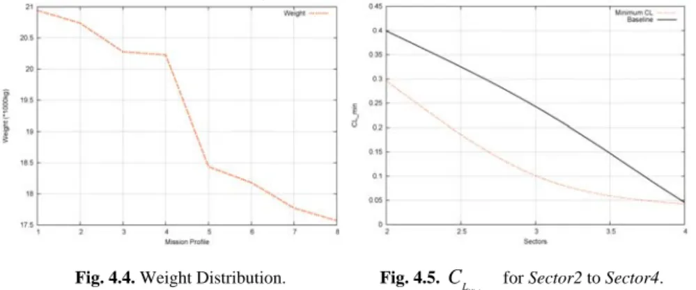
Figure 4.4 shows the weight distribution along the mission profile. The weight be-tween Sector4 and Sector5 is significantly reduced since 80% of munitions weight is used for target strike. In this paper, flight conditions for Sector2 to Sector4 are considered and the minimum lift coefficients (CLmin) are 0.296 and 0.04 for
Sec-tor2 and Sector4 as shown in figure 4.5.
Fig. 4.4. Weight Distribution. Fig. 4.5.
Minimum
L
C for Sector2 to Sector4.
The baseline design produces 30% higher lift coefficient at Sector2 when com-pared to CLmin while only 7% higher at Sector4. The aim of optimisation is the
im-provement of aerodynamic performance at Sector4 while maintaining aerodynam-ic performance in Sector2.
Representation of Design Variables
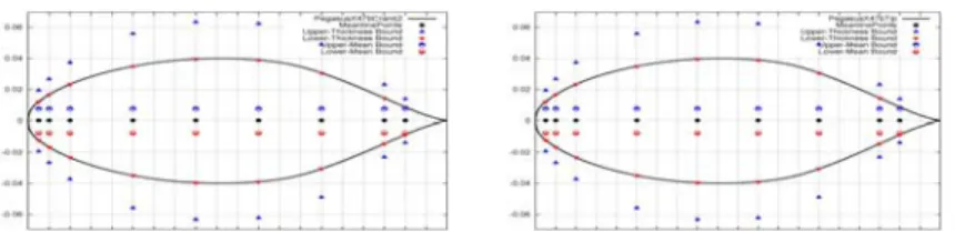
The aerofoil geometry is represented using Bézier curves with a combination of mean line and thickness distribution control points. Example of the upper and lower bounds for mean and thickness control points at root, crank 1, crank 2 and tip sections are illustrated in figures 4.6a and 4.6b.
Fig. 4.6a. Root (left) and Crank1 (right) mean and thickness control points.
Fig. 4.6b. Crank2 (left) and Tip (right) mean and thickness control points.
The wing planform shape is parameterised by considering the variables described in table 4.1 where three wing section areas, three sweep angles and two taper rati-os are considered. The taper ratio at crank 2 is not higher than the taper ratio at crank 1 i.e. (C2C1). Seventy six design variables are considered in total.
Table 4.1. Wing planform design variables.
Variables S1 (m2) S2 (m2) S3 (m2) C1 C2 RC1 C1C2 C2T
Lower 50.46 10.09 5.05 0.15 0.15 49.5 25 25 Upper 63.92 16.82 10.09 0.45 0.45 60.5 35 35
4.1.4 Real World Design Problems
Two real world test cases are selected to illustrate the potential of this methodolo-gy with increasing levels of complexity. The first case considers the aerodynamic analysis and optimisation on a J-UCAV, the second test compares and illustrates the challenge and benefits in industrial environments on introducing a second dis-cipline (electro-magnetics) while accounting for uncertainty in the design parame-ters and operating conditions.
4.1.4.1 Multi-objective Design Optimisation of J-UCAV
Problem DefinitionThis test case considers the design optimisation of a UCAV wing aerofoil sections and planform geometry. The objectives are to maximise both mean values of lift
coefficient (CL) and lift to drag ratio (L D/ ) at Sector2 and Sector4. The fitness
functions and flight conditions are as follows;
1 min 1 / CL f and f2 min 1 /
L D/
where
2 4 2 Mission Mission L L LC C C and L D/ L D/ Mission2L D/ Mission4 2
Results
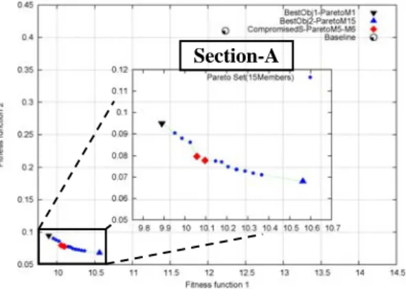
The algorithm was allowed to run approximately for 6667 function evaluations and took 200 hours on two 2.4 GHz processors. The resulting Pareto set is shown in figure 4.7. The black inverse triangle represents the best solution for fitness function 1. The blue triangle indicates the best solutions for the fitness function 2. The red squares represent compromised solutions. It can be seen that there is a convex Pareto front between first and second objective as shown in Section-A.
Fig. 4.7. Pareto optimal front.
Table 4.2 compares the fitness values obtained by the baseline and Pareto mem-bers (1, 5, 6 and 15). It can be seen that all non-dominated solutions produce high-er CL and L D/ . There was a 17.5% of CL and 80% L D/ improvement when
compared to the baseline design.
Table 4.2. Comparison of the objectives.
Description Baseline ParetoM1 ParetoM5 ParetoM6 ParetoM15
1 / CL 12.232 9.890 (-19%) 10.056 (-18%) 10.096 (-17%) 10.562 (-14%)
1 / L D/ 0.410 0.095 (-77%) 0.079 (-80%) 0.078 (-81%) 0.068 (-83%)
The Sector sweep is plotted with CL and CD in figures 4.8a and 4.8b. The range of
Sector sweep (Sector2 to Sector4) is M= [0.7:0.9], = [6.05:0.5] and ATI = [40,000:250].
Fig. 4.8a.CL vs. Sector sweep. Fig. 4.8b.CD vs. Sector sweep.
It can be seen that all Pareto members (1, 5, 6 and 15) produce higher CL when
compared to the baseline. Pareto member 1 indicates higher lift coefficient along all sectors when compared to other solutions while Pareto member 15 has lower drag coefficient from Sector3. In addition, all Pareto members produce lower CD
without fluctuation compared to the baseline design as shown in figure 4.8b. Table 4.3 compares the quality of drag coefficient obtained from Pareto members and the baseline design. It can be seen that all Pareto members produce lower CD
(-60 %) and lower sensitivity at Sector2 to Sector4 when compared to the baseline. Table 4.3. Comparison of CD quality
Description Baseline ParetoM1 ParetoM5 ParetoM6 ParetoM15
D
C 0.025 0.011 (-56%) 0.010 (-60%) 0.009 (-64%) 0.009 (-64%) D
C
5.4910-5 1.4910-5 1.5410-5 1.5610-5 2.1110-5 Figure 4.8c compares the lift to drag ratio obtained by Pareto members (1, 5, 6 and 15) and the baseline design.
It can be seen that all Pareto members produce higher L/D along the Sector sweep which means an extension of flight range. Even though the MO design method found useful Pareto non-dominated solutions produced aerodynamic improvement at Sector2 and Sector4, there is considerable fluctuation of L/D at M
[0.75:0.85] (transition point: Sector2 to Sector3 and Sector3 to Sector4) where a high dash flight is required. Therefore it is necessary to check their aerodynamic quality along the Sector conditions; M [0.75:0.85], [4.662:1.887] and ATI
[30,0062:10,187]. This can be done using mean and variance of L/D; the mean value indicates the scalar of objective while the variance can be interpreted as the stability/sensitivity of objective.
Table 4.4 compares the quality of L/D obtained from the Pareto members and the baseline design. The L/D variances of the optimal solutions are higher than the baseline design. This means Pareto members are over-optimised solutions to max-imise an aerodynamic performance at design conditions.
Table 4.4. Comparison of L/D quality
Description Baseline ParetoM1 ParetoM5 ParetoM6 ParetoM15
L D 10.525 27.62 30.03 31.05 33.222
L D
8.25 23.53 42.08 50.19 127.10
This fluctuation can lead to the structural or control failure at transition point. This fluctuation can be avoided by using robust design technique during optimisation. However, particular care is required for deciding variability of flight conditions. For instance, the variable operating conditions are considered between blue centre lines in figure 4.8c then the variance (Line-B) of the baseline is higher than Pareto member 1 (Line-A) even though the baseline is more stable (low sensitivity) from Sector2 to Sector4 conditions. The introduction of uncertainty with effective vari-ability of operating conditions is implemented in the next subsection to produce stable solutions on both drag coefficient and lift to drag ratio.
4.1.4.2 Uncertainty based MDO of J-UCAV
Problem DefinitionTwo disciplines aerodynamics and electromagnetics are considered to maximise the survivability of the UCAV when operating on a target strike mission. The first objective is to maximise the mean of L/D in the aircraft Sector3 while minimising the second fitness function variance of L/D to reduce fluctuation (Fig. 4.8c) at var-iable flight conditions. A third fitness function considers mono (Sector2) and bi-static (Sector4) radar analysis at variable radar frequency to produce a stealth UCAV. The RCS quality (scalar and stability) is expressed as one combined sta-tistical formula in terms of the mean and variance.
where MS, S, ATIS and FS represents the standard design condition. The fitness functions for this problem are defined as;
1 1 min / fitness f L D
--(mean) and 2 min
L fitness f D --(variance) 3
1 min 2 mono bi Quality mono bi fitness f RCS RCS RCS RCS RCS where 2 2 1 1 i K i i S L D M L D K M
and 2 2 2 1 1 / / 1 K i i i S M L L D L D D K M
where [0 : 3 : 360 ] and [0 : 0 : 0 ] (Mono-static)
where 0 135 , 90 0 at [0 : 3 : 360 ] , [0 : 0 : 0 ] (Bi-static)
Results
The algorithm was allowed to run approximately for 539 function evaluations and took 200 hours on two 2.4 GHz processors.
Fig. 4.9. Pareto optimal front.
The resulting Pareto set is shown in figure 4.9 where the black inverse triangle (Pareto member 1) represents the best solution for fitness function1. The red square (Pareto member 10) represents the best solution for fitness function 2. The blue triangle (Pareto member 10) indicates the best solution for the third fitness. The light blue square (Pareto member 8) indicates the compromised solution. It can be seen all Pareto members produce higher L/D with low sensitivity while their wing planform shapes have low observability.
Table 4.5 compares the mean and variance of lift to drag ratio and RCS quality ob-tained by Pareto members (1, 8, 10) and the baseline design.
Table 4.5. Comparison of the objectives.
Description Baseline ParetoM1 ParetoM8 ParetoM10
1 L D/ 0.095 0.051 (-46%) 0.063 (-34%) 0.078 (-18%)
L D/
8.25 5.35 (-35%) 2.91 (-65%) 2.73 (-67%)
Quality
RCS 80.58 37.29 (-53%) 36.67 (-54%) 33.62 (-58%)
Pareto member 1 produces lower inverse mean lift to drag ratio by 46% with 35% reduction of sensitivity when compared to the baseline design. The sensitivity
(L/D) of Pareto member 10 is lower by 67% with 18% improvement in 1 L D/ . These indicate that all Pareto members produce higher aerodynamic performance with less sensitivity at the start of Sector3 to end of Sector3 where the fluctuation is shown in figure 4.8c. In addition all Pareto members have RCS quality im-provement (more than 50%) when compared to the baseline design.
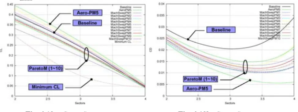
Figures 4.10a -c compare the Sector sweep vs. CL, CD and L/D obtained from
cur-rent non-dominated solutions (Pareto members 1~10), Pareto member 5 (denoted as AeroPM5) from previous test (section 5.1) and the baseline design. The range of Sector sweep is from Sector2 to Sector4. Figure 4.10a shows that the current Pareto members (1 and 2) and AeroPM5 produce higher CL along the Sector
sweep when compared to the baseline design. Pareto members (3 to 10) have a lower CLwhen compared to the baseline design while having a higher CL value
than CLmin.
Fig. 4.10a.CL vs. Sector sweep. Fig. 4.10b.CD vs. Sector sweep.
Figure 4.10b and table 4.6 compare the mean and sensitive of CD obtained by
Pa-reto members (1 to 10), AeroPM5 and the baseline design. AeroPM5 produces lower drag when compared to the other Pareto members and the baseline, whereas the current Pareto members have much lower CD sensitivity along the Sector
D
C
5.4910 1.5410 7.91710 6.4810 3.8310
Figure 4.10c compares the L/D along the Sector sweep obtained by Pareto mem-bers (1 to 10), AeroPM5 from previous test and the baseline design. It can be seen that Pareto member 1 and AeroPM5 produce higher L/D than the baseline design while Pareto member 10 produces lower sensitivity. It can be seen that one of the benefit of uncertainty design technique is that the maximum L/D point (Point-A) of AeroPM5 moves to the maximum L/D point (Point-B) of Pareto member 1 and then the designs and solutions moves to Point-C of Pareto member 10 which cor-responds to and reflects the variance.
Fig. 4.10c.L/D vs. Sector sweep.
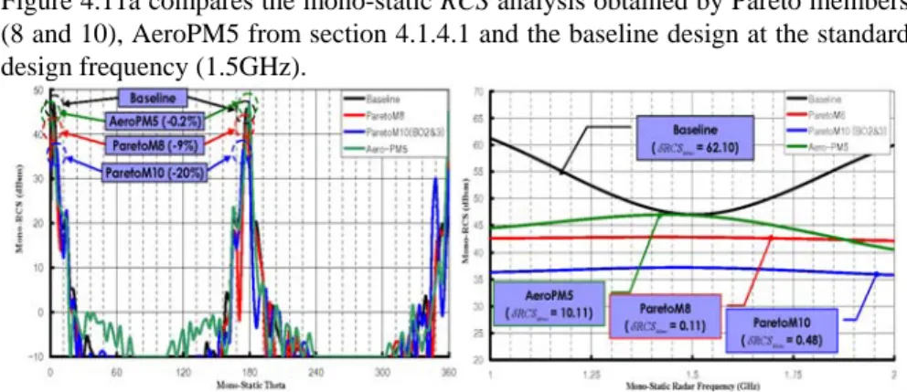
Figure 4.11a compares the mono-static RCS analysis obtained by Pareto members (8 and 10), AeroPM5 from section 4.1.4.1 and the baseline design at the standard design frequency (1.5GHz).
It can be seen that Pareto members 8 and 10 produce 9% and 20% lower RCS when compared to the baseline design while AeroPM5 produces almost the same RCS as the baseline design. Figure 4.11b illustrates a frequency sweep corre-sponding to mono-static RCS analysis. The variance value for Pareto member 8 is lower while the baseline design value highly fluctuates at the standard design ra-dar frequency (1.5GHz).
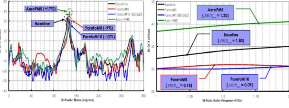
Fig. 4.12a.RCSBi at standard frequency. Fig. 4.12b.RCSBi vs. FBi-static.
Figure 4.12a compares the bi-static RCS analysis obtained by Pareto members (8 and 10), AeroPM5 and the baseline design at the standard deign frequency (1.5GHz). Even though AeroPM5 produces higher aerodynamic performance, its bi-static RCS indicates that it has 17% more chance to be detected to enemy radar system when compared to the baseline design. Pareto members 8 and 10 have 9% and 12% lower observability when compared to the baseline design. Figure 4.12b compares the bi-static RCS at variable frequencies and shows the lowest RCS vari-ance is achieved by Pareto member 10 (RCSBI= 0.09).
4.1.5 Conclusions
A new methodology for the design and optimisation of UCAV aerofoil sections and wing planform shapes have been proposed and investigated numerically. The methodology couples a robust multidisciplinary evolutionary algorithm, with aer-odynamic and RCS analysis software. The results of the method show that by in-troducing another discipline and a robust design analysis it is possible to compute a set of useful Pareto non-dominated solutions that produces 55% lower sensitivity and 35% higher aerodynamic performance with 55% lower observability at varia-ble flight conditions and radar frequencies when compared to the baseline design. Future work will focus on coupling the method with other game strategies such as Nash and hierarchical game. Results obtained from different games will be com-pared in terms of efficiency and design quality in a forthcoming paper.
The 5th Asian Computational Fluid Dynamics. Busan, Korea.
[3] Tang Z, Périaux J. and Désidéri J-A (2005) Multi Criteria Robust Design Using Adjoint Methods and Game Strategies for Solving Drag Optimization Problems with Uncertainties, in: East West High Speed Flow Fields Conference 2005, p. 487-493.
[4] Trosset MW (2004) Managing Uncertainty In Robust Design Optimisation. Lecture note, Department of Mathematics College of William & Mary.
[5] Lee DS, Gonzalez LF, Srinivas Kand Periaux J (2008)Robust Evolutionary Algorithms for UAV/UCAV Aerodynamic and RCS Design Optimisation, Special Issue of Computers and Fluids dedicated to Prof. M. Hafez. Vol 37. Issue 5, pages 547-564, ISSN 0045-7930. [6] Lee DS, Gonzalez LF, Srinivas Kand Periaux J (2008) Robust Design Optimisation using
Multi-Objective Evolutionary Algorithms, Special Issue of Computers and Fluids dedicated to Prof. M. Hafez. Vol 37. Issue 5, pages 565-583, ISSN 0045-7930.
[7] Lee DS, Gonzalez LF and Whitney EJ (2007) objective, Multidisciplinary Multi-fidelity Design tool: HAPMOEA – User Guide.
[8] Koza J (1994) Genetic Programming II. Massachusetts Institute of Technology.
[9] Michalewicz Z (1992) Genetic Algorithms + Data Structures = Evolution Programs. Artifi-cial Intelligence, Springer-Verlag.
[10] Hansen N and Ostermeier A (2001) Completely Derandomized Self-Adaptation in Evolu-tion Strategies. EvoluEvolu-tionary ComputaEvolu-tion, 9(2), pp. 159-195.
[11] Hansen N, Müller SD and Koumoutsakos P (2003) Reducing the Time Complexity of the Derandomized Evolution Strategy with Covariance Matrix Adaptation (CMA-ES). Evolu-tionary Computation, 11(1), pp. 1-18.
[12] Sefrioui M and Périaux J (2000) A Hierarchical Genetic Algorithm Using Multiple Models for Optimization. In M. Schoenauer, K. Deb, G. Rudolph, X. Yao, E. Lutton, J.J. Merelo and H.-P. Schwefel, editors, Parallel Problem Solving from Nature, PPSN VI, pages 879-888, Springer.
[13] Wakunda J. and Zell A (2000) Median-selection for parallel steady-state evolution strate-gies. In Marc Schoenauer, Kalyanmoy Deb, Günter Rudolph, Xin Yao, Evelyne Lutton, Juan Julian Merelo, and Hans-Paul Schwefel, editors, ParallelProblem Solving from Nature – PPSN VI, pages 405–414, Berlin, Springer.
[14] Veldhuizen D, Van A, Zydallis JB, and Lamont GB (2003) Considerations in Engineering Parallel Multiobjective Evolutionary Algorithms, IEEE Transactions on Evolutionary Com-putation, Vol. 7, No. 2, pp. 144--173.
[15] Trosset MW (2004) Managing Uncertainty In Robust Design Optimisation. Lecture note, Department of Mathematics College of William & Mary.