Spin–orbit effects in the bismuth atom and dimer: tight-binding and density functional theory
comparison
This article has been downloaded from IOPscience. Please scroll down to see the full text article.
2013 J. Phys. B: At. Mol. Opt. Phys. 46 095101
(http://iopscience.iop.org/0953-4075/46/9/095101)
Download details:
IP Address: 130.104.231.222
The article was downloaded on 28/05/2013 at 10:43
Please note that terms and conditions apply.
View the table of contents for this issue, or go to the journal homepage for more
J. Phys. B: At. Mol. Opt. Phys.46(2013) 095101 (9pp) doi:10.1088/0953-4075/46/9/095101
Spin–orbit effects in the bismuth atom
and dimer: tight-binding and density
functional theory comparison
Micael J T Oliveira
1,2and Xavier Gonze
2,31 Center for Computational Physics, University of Coimbra, Rua Larga, 3004-516 Coimbra, Portugal 2European Theoretical Spectroscopy Facility (ETSF)
3 Universit´e Catholique de Louvain, IMCN/NAPS, Louvain-la-Neuve, Belgium E-mail:[email protected]
Received 29 November 2012, in final form 17 March 2013 Published 16 April 2013
Online atstacks.iop.org/JPhysB/46/095101 Abstract
We present a simple tight-binding model for the bismuth atom and dimer whose main feature is the inclusion of the spin–orbit coupling in such a way that it allows the study of several electronic properties as a function of the spin–orbit coupling strength. Density functional theory calculations (norm-conserving and full-potential linearized augmented plane wave) are used to obtain the tight-binding parameters and to check the accuracy of the model. The model is then used to show in a straightforward way that, in the case of the bismuth dimer, the inclusion of the spin–orbit coupling produces a set of molecular orbitals that are a mixture of bonding and non-bonding non-relativistic molecular orbitals, thus weakening the molecular bond.
(Some figures may appear in colour only in the online journal)
1. Introduction
A proper account of relativistic effects is essential for an accurate determination of the electronic properties of systems including heavy elements. In the past decades, a great amount of work has been devoted to understanding what is the effect of considering relativity with respect to the results obtained from the simpler and more widely used non-relativistic theory. For example, it has been known for quite some time that gold is predicted to be yellow only if relativistic effects are taken into account [1]. More recently, it was shown that relativistic effects are responsible for the unique bonding pattern of U2 [2]. Other studies also showed the importance of relativistic effects in systems like nanographene [3] or organo-transition metal compounds [4]. Many other examples can be found in the literature of how electronic properties, like bond lengths, dissociation energies, photo-electron spectra, etc, are predicted to be different if relativistic effects are taken into account (see e.g. [1,5,6] and references therein).
Because of its large atomic number (Z = 83), bismuth is a clear case where relativistic effects cannot be ignored. Moreover, crystalline bismuth exhibits quite
interesting properties. For example, it is the most diamagnetic elemental solid [7] and is considered to be an ideal system to study quantum confinement effects [8, 9]. Recently, it was shown that the inclusion of the spin–orbit coupling is essential to obtain phonon band structures and specific heat of crystalline bismuth in agreement with experiment [10,11]. In particular, ab initio calculations of the specific heat of bismuth were carried with the spin–orbit coupling term multiplied by a parameter that was used to vary the spin–orbit strength. This was done in an attempt to better understand what was the impact of this relativistic effect when determining the thermodynamic properties of crystals. Besides the bulk, bismuth nanostructures, like nanotubes, nanowires and clusters, have also attracted some attention [12–14]. In particular, the bismuth dimer has been studied to some extent theoretically and experimentally [15, 16]. Concerning the importance of relativistic effects, van Lenthe et alanalysed the effect of spin–orbit coupling on the electronic properties of the dimer using the ZORA Hamiltonian within density functional theory (DFT) [17]. They showed that, although the bond length of the dimer only changed by 1% when spin–orbit coupling was included, the dissociation energy
J. Phys. B: At. Mol. Opt. Phys.46(2013) 095101 M J T Oliveira and X Gonze decreased by almost 40%. This weakening of the bond is
quite significant. For example, it is partially responsible for the changes observed in the phonon band structure of the bulk [11]. A simple qualitative explanation for this change in the bond was given by Pitzer, who argued that the j j coupled relativistic p orbitals of the atom could not combine to form good bonding molecular orbitals [18,19,1].
Nowadays, relativistic effects can be readily included in ab initio calculations, like quantum chemistry methods or DFT. Nevertheless, understanding how relativity affects the properties of atoms, molecules or solids in ab initio
calculations is not always straightforward. Furthermore, calculations including heavy atoms can be very CPU intensive, such that many systems of interest are out of reach from today’s available computational power. On the other hand, tight-binding models [20] are usually much cheaper from the computational point of view and the simplicity of the tight-binding Hamiltonian makes it easier to understand the contribution of specific terms like the spin–orbit coupling. The inclusion of spin–orbit coupling in tight-binding models was proposed some years ago [21] and one can even find such a model for bulk bismuth [22]. However, to our knowledge, there is no similar model for the bismuth dimer nor an analysis of the effect of spin–orbit coupling on the dimer bond length based on such a model.
In this work we introduce tight-binding models for the bismuth atom and dimer that include the spin–orbit coupling. In these models, a parameter is introduced to control the strength of the spin–orbit coupling, such that it is possible to study the change in the electronic properties when the spin–orbit coupling is switched on and is increased up to full strength. We also performed DFT calculations where the spin–orbit coupling term was included multiplied by a similar parameter as in the tight-binding models. The details of the DFT calculations are presented in section2. The tight-binding models are presented in section3. In section4, we discuss how to fit the tight-binding parameters using the DFT results and compare the results obtained with both methods. We finalize by using the tight-binding model to analyse the effect of the spin–orbit coupling on the bond length of the bismuth dimer.
2.
Ab initio
calculations
We have performed calculations of the eigenvalues of the bismuth atom and dimer within DFT [23]. The core electrons were treated using norm-conserving pseudopotentials. Since most relativistic effects come from the core electrons, these have to be taken into account in the pseudopotential. This is done starting from all-electron fully relativistic calculations for the atom and by generating the pseudopotentials using a suitable scheme. In this work, we decided to use pseudopotentials generated from the scheme of Hartwigsen, Goedecker and Hutter (HGH) [24] and the relativistic extension of the Troullier–Martins (TM) scheme [25, 26]. For reasons of computational efficiency, pseudopotentials are usually applied in a fully non-local form [27]. In the case of relativistic pseudopotentials including spin–orbit, there are two ways of expressing them in a non-local form. In the first
case, the pseudopotentials are written in terms of scalar-relativistic and spin–orbit coupling terms,VSR
l andVlSO, and
depend on the angular momentum quantum numberl. This in turns allows us to express the projectors in terms of the spin and angular momentum eigenfunctions [28]:
VPP(r,r)=Vloc(r)δ(r−r)+ ls VlSR(r,r)|lsls| + ls VlSO(r,r)Lˆ · ˆS|lsls|, (1)
whereVlocis the local part of the potential. This means that, in this case, the strength of the spin–orbit coupling can be controlled by simply multiplying the third term of (1) by a parameterλ. In the second case, the pseudopotentials depend on the total angular momentum quantum number j and the projectors are written in terms of the total angular momentum eigenfunctions [29]:
VPP(r,r)=Vloc(r)δ(r−r)+
j
Vj(r,r)|jj|. (2)
Although the spin–orbit term does not appear explicitly in (2), it is nevertheless possible to rewrite the projectors in terms of the Pauli matrices and thus identify the spin–orbit term and multiply it byλ [30]. The HGH pseudopotentials are generated directly in the form of (1), while for the TM scheme,j-dependent pseudopotentials are first generated in a semi-local form and later they can be either transformed into (1) or into (2) [27–29,31].
The HGH pseudopotential for bismuth used in this work was taken directly from [24], while a relativistic TM pseudopotential was generated using the APE package [32]. As for the actual DFT calculations for the atom and dimer, we used theOCTOPUS[33] and ABINIT [34] computer codes. ABINIT allows for the usage of HGH pseudopotentials and relativistic TM pseudopotentials expressed as in (1). HGH pseudopotentials can also be used withOCTOPUS, while relativistic TM pseudopotentials are handled using (2). In both codes the valence electrons are treated with the non-relativistic Schr¨odinger equation. This is a very good approximation, as the Dirac equation for the valence states outside the core region reduces to the non-relativistic Schr¨odinger equation.
As a further validation step of our ab initio results, we calculated the atom and dimer eigenvalues with an all-electron method. In particular, we used the full-potential linearized augmented plane wave (FP-LAPW) method [35] as implemented in the ELK code [36]. In this method, the spin–orbit coupling is included as a perturbation within the second-variational scheme, so it is straightforward to multiply it by a parameterλ.
All the calculations were performed using the Perdew– Wang parametrization of the local density approximation [37] for the exchange and correlation functional.
In OCTOPUS the wavefunctions are discretized in a real-space grid and zero-boundary conditions are used when dealing with finite systems. As such, there are basically two parameters that control the convergence: the grid spacing and the size of the box that contains the system. We found that a spacing of 0.52 au and a sphere of radius 11.5 au was necessary to converge the 6p eigenvalues of the bismuth atom to less than 2
-0.24 -0.22 -0.2 -0.18 -0.16 -0.14 -0.12 0 0.2 0.4 0.6 0.8 1 Eigenvalues (a.u.) Spin-orbit strength TM - ABINIT HGH - ABINIT TM - octopus HGH - octopus FP-LAPW
Figure 1.Ab initioeigenvalues of the 6p states of the bismuth atom as a function of the spin–orbit strength computed using the FP-LAPW method and using TM and HGH pseudopotentials. a millihartree for all pseudopotentials. The same spacing was used for the bismuth dimer, but in this case the simulation box was built by taking two spheres of radius 11.5 au centred around each atom. In the case of ABINIT, the wavefunctions are expanded in a plane-wave basis set and periodic boundary conditions are used in all cases. We found that an energy cut-off of 10 Ha and a super-cell of 50×50×50 au was necessary to fulfil the same convergence criteria. As for the FP-LAPW calculations, the radius of the muffin-tin spheres, RMT, was chosen to be 2.4 au, so that there were no overlapping spheres in our calculations. The plane-wave cut-off,kmax, was chosen such thatRMTkmax=7.0. Finally, the size of the super-cell used was the same as for the ABINIT calculations.
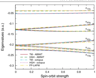
In figure1, we plot the 6p eigenvalues of the bismuth atom as a function of the spin–orbit coupling strengthλcalculated with ELK, and withOCTOPUSand ABINIT using TM and HGH pseudopotentials. In this case, all the curves corresponding to the pseudopotential calculations are very close to each other. The only noticeable difference occurs for the eigenvalues of the three unoccupied 6p states, which are slightly shifted upwards in the case of the ABINIT calculation. We note that this shift occurs even without spin–orbit coupling and that these curves are the most difficult to converge with respect to the size of the box, so this difference is not surprising and is within the expected numerical error. More important than this shift is the fact that the shape of the curves is identical in all cases. As for the FP-LAPW curves, we note small deviations from the pseudopotential curves for larger values ofλ. This is probably because of the different way in which the spin–orbit coupling is handled in the FP-LAPW method. In figure2, we plot the same curves, but for the eigenvalues of the bismuth dimer at the experimental bond length of 2.661 ˚A [38]. In this case the curves also exhibit a similar behaviour. The only significant difference is found in the unoccupied antibonding
σ1/2uorbital eigenvalues obtained using TM pseudopotentials,
which differ from the other curves by more than 0.01 Ha. Because the results obtained with the TM pseudopotentials are very similar for the two codes, the differences must come
-0.3 -0.25 -0.2 -0.15 -0.1 -0.05 0 0.2 0.4 0.6 0.8 1 Eigenvalues (a.u.) Spin-orbit strength σ1/2u π3/2g π1/2g π3/2u π1/2u σ1/2g TM - ABINIT HGH - ABINIT TM - octopus HGH - octopus FP-LAPW
Figure 2.Ab initioeigenvalues of the bondingσ1/2g,π1/2uandπ3/2u molecular orbitals and of the antibondingσ1/2u,π1/2gandπ3/2g molecular orbitals of the bismuth dimer as a function of the spin–orbit strength computed using the FP-LAPW method and using TM and HGH pseudopotentials. Note that each state is doubly degenerate.
from the pseudopotential. However, we can rule out the way in which the spin–orbit coupling is handled as a possible cause for these differences, as they occur even when there is no spin– orbit coupling, i.e. whenλ=0. Despite these differences, we note that the shape of all the curves is the same, even more than in the case of the atom. Thus, in the remainder of this work we will only use theab initioresults obtained with one of the codes and pseudopotentials (OCTOPUSwith TM pseudopotential).
3. Tight-binding model
3.1. Bismuth atom
The basis functions for the tight-binding model are taken to be the scalar-relativistic spin-dependent wavefunctions of the 6p orbitals of the bismuth atom in its ground-state configuration ([Xe]4f145d106s26p3): ψ↑ 6,1,1(r)↑ =R↑6,1(r)Y11(θ, φ)| ↑, (3) ψ↑ 6,1,0(r)↑ =R↑6,1(r)Y10(θ, φ)| ↑, (4) ψ↑ 6,1,−1(r)↑ =R↑6,1(r)Y1−1(θ, φ)| ↑, (5) ψ↓ 6,1,1(r)↓ =R↓6,1(r)Y11(θ, φ)| ↓, (6) ψ↓ 6,1,0(r)↓ =R↓6,1(r)Y10(θ, φ)| ↓, (7) ψ↓ 6,1,−1(r)↓ =R↓6,1(r)Y1−1(θ, φ)| ↓, (8)
where we have separated the wavefunctions in radial, angular and spin parts in the usual way.
The Hamiltonian of the system is
ˆ
J. Phys. B: At. Mol. Opt. Phys.46(2013) 095101 M J T Oliveira and X Gonze whereHˆatis the scalar-relativistic atomic Hamiltonian, and the
spin–orbit coupling termHˆsocan be written as ˆ
Hso=ξ (r)Lˆ· ˆS. (10)
At this point, in the same spirit as in the previous section, we introduce the parameterλthat controls the strength of the spin–orbit coupling:
ˆ
H= ˆHat+λHˆso. (11) When λ = 1, we recover the usual form of the spin–orbit interaction, while setting λ = 0 is equivalent to neglect the spin–orbit coupling. The Bi atom (with 3p electrons at
λ=0) is spin-polarized, following Hund’s rule. Accordingly, we distinguish the spin up↑ and spin down↑ eigenvalues (and associated eigenvectors).
The next step is to find the solutions of the Schr¨odinger equation:
ˆ
H|ψλ =λ|ψλ, (12) where the wavefunction|ψλis expanded in terms of the basis functions: |ψλ(r) = σ=↑,↓ 1 m=−1 cσ,mψ6,1,σ m(r) , σ . (13)
The matrix elementsi| ˆH|jcan easily be determined either by writing the basis functions in terms of total angular momentum states [21] or by writingLˆ · ˆSin terms of ladder operators. In either case, we obtain the following matrix elements for the spin–orbit term: HSO= ⎛ ⎜ ⎜ ⎜ ⎜ ⎜ ⎜ ⎜ ⎜ ⎝ α↑↑ 2 0 0 0 0 0 0 0 0 √ 2α↑↓ 2 0 0 0 0 −α↑↑ 2 0 √ 2α↑↓ 2 0 0 √ 2α↑↓ 2 0 − α↓↓ 2 0 0 0 0 √ 2α↑↓ 2 0 0 0 0 0 0 0 0 α2↓↓ ⎞ ⎟ ⎟ ⎟ ⎟ ⎟ ⎟ ⎟ ⎟ ⎠ , (14)
where we have defined
α↑↑=R↑6,1(r)|ξ (r)|R↑6,1(r) , (15) α↓↓=R↓6,1(r)|ξ (r)|R↓6,1(r) , (16) α↑↓=α↓↑=R↑6,1(r)|ξ (r)|R↓6,1(r) . (17)
The eigenvalues are determined in the usual way by solving the secular equation, giving
1 λ= 1 2 ↑+↓−λα↑↑ 2 −1 2 ↓−↑+λα↑↑ 2 2 +2λ2α↑↓2 1 2 , (18a) 2 λ= 1 2 ↑+↓−λα2↑↑ +1 2 ↓−↑+λα↑↑ 2 2 +2λ2α↑↓2 1 2 , (18b) 3 λ=↑+λα↑↑ 2 (18c) 4 λ= 1 2 ↑+↓−λα↓↓ 2 −1 2 ↑−↓+λα2↓↓ 2 +2λ2α2↑↓ 1 2 , (18d) 5 λ= 1 2 ↑+↓−λα↓↓ 2 +1 2 ↑−↓+λα↓↓ 2 2 +2λ2α2↑↓ 1 2 , (18e) 6 λ=↓+λα↓↓ 2 , (18f)
where↑and↓are the eigenvalues ofHˆat.
The case where the states with opposite spins are equally occupied, like closed-shell atoms, is a particular case of the previous equations. Indeed, in that case we have R↑(r) = R↓(r)and↑=↓=p, and the eigenvalues are given by
1,4
λ =p−λα , (19a)
λ2,3,5,6=p+λα , (19b)
withα↑↑=α↑↓=α↓↓=α.
3.2. Bismuth dimer
At the equilibrium bond length, the bismuth dimer is non-magnetic, i.e. the magnetization density is null everywhere in space. As such, we will use the wavefunctions of the non-magnetic atom as basis functions. Therefore, the wavefunctions of our basis corresponding to the first atom are |ψ6,1,1(r−R1)↑, (20) |ψ6,1,0(r−R1)↑, (21) |ψ6,1,−1(r−R1)↑, (22) |ψ6,1,1(r−R1)↓, (23) |ψ6,1,0(r−R1)↓, (24) |ψ6,1,−1(r−R1)↓, (25) and the wavefunctions corresponding to the second atom are
|ψ6,1,1(r−R2)↑, (26) |ψ6,1,0(r−R2)↑, (27) |ψ6,1,−1(r−R2)↑, (28) |ψ6,1,1(r−R2)↓, (29) 4
|ψ6,1,0(r−R2)↓, (30) |ψ6,1,−1(r−R2)↓, (31) whereR1andR2are the positions of the two bismuth atoms.
The Hamiltonian of the system can be written as
ˆ
H= ˆHat(1)+λHˆso(1)+ ˆHat(2)+λHˆso(2)+Vˆ, (32) where Hˆat(i) is the Hamiltonian of an isolated atom, Vˆ is the interaction between the two atoms,Hˆ(i)
so is the spin–orbit coupling acting on one atom, and we have again introduced a parameterλthat controls the spin–orbit coupling strength.
Like for the case of the atom, we search solutions of (12), and the wavefunctions are again expanded in terms of the basis functions: |ψλ(r) = 2 i=1 σ=↑,↓ 1 m=−1 c(σ,i)m|ψ6,1,m(r−Ri) , σ. (33)
As for the determination of the matrix elements, we will consider that the only contributions of Hˆat(i) andHˆ(i)
so are the ones involving basis functions centred on atomi. This implies that the only non-zero integrals involving two centres are the ones concerning the interaction between the two atomsVˆ. Taking this into account, we can write the matrix elements as
H= A B B A , (34)
whereAandBare
A= ⎛ ⎜ ⎜ ⎜ ⎜ ⎜ ⎜ ⎜ ⎝ p+λα2 0 0 0 0 0 0 p 0 √ 2λα 2 0 0 0 0 p−λα2 0 √ 2λα 2 0 0 √22λα 0 p−λα2 0 0 0 0 √ 2λα 2 0 p 0 0 0 0 0 0 p+λα2 ⎞ ⎟ ⎟ ⎟ ⎟ ⎟ ⎟ ⎟ ⎠ , (35) B= ⎛ ⎜ ⎜ ⎜ ⎜ ⎜ ⎜ ⎝ Vπ 0 0 0 0 0 0 Vσ 0 0 0 0 0 0 Vπ 0 0 0 0 0 0 Vπ 0 0 0 0 0 0 Vσ 0 0 0 0 0 0 Vπ ⎞ ⎟ ⎟ ⎟ ⎟ ⎟ ⎟ ⎠ , (36)
and where we have made
ψ6,1,1(r−R1)↑ |Vˆ|ψ6,1,1(r−R2)↑ =Vπ, (37) ψ6,1,1(r−R1)↓ |Vˆ|ψ6,1,1(r−R2)↓ =Vπ, (38) ψ6,1,0(r−R1)↑ |Vˆ|ψ6,1,0(r−R2)↑ =Vσ, (39) ψ6,1,0(r−R1)↓ |Vˆ|ψ6,1,0(r−R2)↓ =Vσ, (40) ψ6,1,−1(r−R1)↑ |Vˆ|ψ6,1,−1(r−R2)↑ =Vπ, (41) ψ6,1,−1(r−R1)↓ |Vˆ|ψ6,1,−1(r−R2)↓ =Vπ. (42) This choice for the integrals of two centres just corresponds to fixing the axis of the dimer along a given direction in space.
Like for the case of the atom, the eigenvalues of the dimer are obtained by solving the secular equation. The solutions are readily obtained and are the following:
1= p− 1 2 λα 2 +Vσ+Vπ +1 2 λα 2 −Vσ+Vπ 2 +2λ2α2 1 2 , (43a) 2= p− 1 2 λα 2 −Vσ−Vπ −1 2 λα 2 +Vσ−Vπ 2 +2λ2α2 1 2 , (43b) 3= p+ λα 2 +Vπ, (43c) 4= p− 1 2 λα 2 +Vσ+Vπ −1 2 λα 2 −Vσ+Vπ 2 +2λ2α2 1 2 , (43d) 5= p+λα 2 −Vπ, (43e) 6= p− 1 2 λα 2 −Vσ−Vπ +1 2 λα 2 +Vσ−Vπ 2 +2λ2α2 1 2 . (43f)
Note that all eigenvalues are twofold degenerate.
When there is no spin–orbit coupling, we recover well-known solutions for the tight-binding model of a non-magnetic dimer. Indeed, whenλ=0, the previous solutions become
1 λ=0=p−Vσ, (44a) 2,3 λ=0 =p+Vπ, (44b) λ=4,50=p−Vπ, (44c) 6 λ=0=p+Vσ. (44d)
From the previous equations, one sees that the tight-binding model predicts the eigenvalues of the bonding and antibonding orbitals to be symmetric with respect topwhen
λ= 0. Considering that from the DFT calculations we have
p = −0.176 au, we immediately see from figure2that this
symmetry is not respected by the DFT results, especially in the case of theσ orbitals. Since our purpose focuses on the behaviour with respect to the spin–orbit strength, we will allow some modification of this model at λ = 0 to correct this problem, that will then simply be transferred to the non-zero
λcase. First, the value ofpwill be different in the dimer and
J. Phys. B: At. Mol. Opt. Phys.46(2013) 095101 M J T Oliveira and X Gonze -0.24 -0.22 -0.2 -0.18 -0.16 -0.14 -0.12 0 0.2 0.4 0.6 0.8 1 Eigenvalues (a.u.) Spin-orbit strength DFT Tight-binding -0.24 -0.22 -0.2 -0.18 -0.16 -0.14 -0.12 0 0.2 0.4 0.6 0.8 1 Eigenvalues (a.u.) Spin-orbit strength DFT Tight-binding
Figure 3.Eigenvalues of the 6p states of the bismuth atom as a function of the spin–orbit strength from DFT calculations and calculated with the tight-binding model for magnetic (upper panel) and non-magnetic (lower panel) cases.
the potential due to the redistribution of charge density. Then, we will also take into account the influence of the presence of otherσ andπ orbitals, by allowing a shift of the first and sixth orbitals (σ-like atλ =0) with respect to the second to fifth orbitals (π-like atλ =0). This amounts to replacingp
in equations (43a)–(43f) by two new parameterspandp:
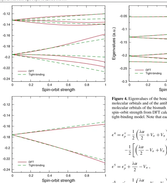
1= p− 1 2 λα 2 +Vσ+Vπ +1 2 λα 2 −Vσ+Vπ 2 +2λ2α2 1 2 , (45a) 2= p− 1 2 λα 2 −Vσ−Vπ −1 2 λα 2 +Vσ−Vπ 2 +2λ2α2 1 2 , (45b) 3= p+ λα 2 +Vπ, (45c) -0.3 -0.25 -0.2 -0.15 -0.1 -0.05 0 0.2 0.4 0.6 0.8 1 Eigenvalues (a.u.) Spin-orbit strength σ1/2u π3/2g π1/2g π3/2u π1/2u σ1/2g DFT Tight-binding
Figure 4.Eigenvalues of the bondingσ1/2g,π1/2uandπ3/2u molecular orbitals and of the antibondingσ1/2u,π1/2gandπ3/2g molecular orbitals of the bismuth dimer as a function of the spin–orbit strength from DFT calculations and calculated with the tight-binding model. Note that each state is doubly degenerate.
4= p− 1 2 λα 2 +Vσ+Vπ −1 2 λα 2 −Vσ+Vπ 2 +2λ2α2 1 2 , (45d) 5= p+ λα 2 −Vπ, (45e) 6= p− 1 2 λα 2 −Vσ−Vπ +1 2 λα 2 +Vσ−Vπ 2 +2λ2α2 1 2 , (45f)
and we obtain the following solutions whenλ=0:
1 λ=0=p−Vσ, (46a) 2,3 λ=0=p+Vπ, (46b) 4,5 λ=0=p−Vπ, (46c) 6 λ=0=p+Vσ. (46d)
4. Tight-binding versus
ab initio
To be able to compare the results obtained using the tight-binding model presented in section3with theab initiodata, it is first necessary to fit the parameters of the model to the
ab initioresults.
A simple way to do this is to take the analytical solutions of the secular equations and use them to write the parameters as functions of the eigenvalues and ofλ. Then one can obtain 6
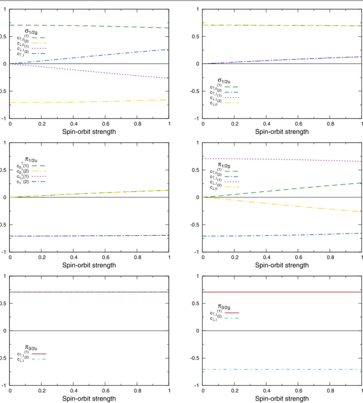
-1 -0.5 0 0.5 1 0 0.2 0.4 0.6 0.8 1 Spin-orbit strength σ1/2g c↑,0(1) c↓,0(2) c↓,1(1) c↑,1(2) -1 -0.5 0 0.5 1 0 0.2 0.4 0.6 0.8 1 Spin-orbit strength σ1/2u c↑,0(1) c↑,1(2) c↓,1(1) c↓,0(2) -1 -0.5 0 0.5 1 0 0.2 0.4 0.6 0.8 1 Spin-orbit strength π1/2u c0↑(1) c0↓(2) c1↓(1) c1↑(2) -1 -0.5 0 0.5 1 0 0.2 0.4 0.6 0.8 1 Spin-orbit strength π1/2g c↑,0(1) c↑,1(2) c↓,1(1) c↓,0(2) -1 -0.5 0 0.5 1 0 0.2 0.4 0.6 0.8 1 Spin-orbit strength π3/2u c↑,1(1) c↓,1(2) -1 -0.5 0 0.5 1 0 0.2 0.4 0.6 0.8 1 Spin-orbit strength π3/2g c↑,1(1) c↓,1(2) Figure 5.Coefficientsc(i)
σ,mof the bondingσ1/2g,π1/2uandπ3/2umolecular orbitals and of the antibondingσ1/2u,π1/2gandπ3/2gmolecular orbitals of the bismuth dimer as a function of the spin–orbit strength. For clarity, only the non-zero values are plotted and indicated in the key. Note that all the orbitals are twofold degenerate, but only the coefficients corresponding to one of the solutions are shown.
the parameters by replacing the eigenvalues by theirab initio
values for a given value ofλ. TheV,pandp parameters of
the bismuth dimer tight-binding model can indeed be obtained this way by considering the case when λ = 0, i.e. by using equations (46a)–(46d). As there are four equations and four parameters, the later can be determined exactly from the
ab initiovalues. Unfortunately, the same cannot be done for the
αparameters. Indeed, a closer inspection of equations (18a)–
(18f) reveals that there is more than one way to write each parameter in terms of the eigenvalues. This is no surprise, as there are more eigenvalues than parameters. If the tight-binding model was able to exactly reproduce all theab initio
eigenvalues at the same time, then the values of the parameters would not depend on which conditions are chosen to be fulfilled. Unfortunately, this is not necessarily the case (and indeed it is not).
J. Phys. B: At. Mol. Opt. Phys.46(2013) 095101 M J T Oliveira and X Gonze Another possible approach to obtain theαparameters is
to fit them in order to minimize the deviations between the
ab initioand tight-binding eigenvalues for a givenλ. Because this approach is more general and might be better suited for practical applications, it is the one that we chose to obtain the
αparameters.
We started by fitting theαparameters for the tight-binding models for the bismuth atom presented in section3using the DFT eigenvalues at λ = 1.0, for both magnetic and non-magnetic cases. This was done by minimizing the average deviation of the tight-binding eigenvalues with respect to the DFT eigenvalues. The minimization was carried out using the Simplex algorithm of Nelder and Mead [39] and the parameters were constrained to positive values. The resulting parameters for the magnetic atom wereα↑↑=0.0581 au,α↑↓=0.0230 au andα↓↓=0.0243 au, with an average deviation of 0.0068 au and a maximum deviation of 0.0091 au. As for the non-magnetic case, we obtainedα=0.0475 au, with an average deviation of 0.0044 au and a maximum deviation of 0.0045 au. In figure3, we plot the curves obtained with these parameters for the 6p eigenvalues compared to the DFT curves. From these plots we see that, although the general trend of the curves is well described in both cases, significant deviations are observed for some eigenvalues in the magnetic case. These deviations increase withλ, while they are very small for small values ofλ, indicating that for this system the full spin–orbit coupling cannot be accurately treated as a perturbation.
Next, we used equations (46a)–(46d) to determine the
V, p andp parameters of the bismuth dimer tight-binding
model. We obtained the following values:p= −0.1386 au,
p = −0.1666 au,Vπ = −0.0364 au andVσ = 0.0857 au.
As for theαparameter, we used the one obtained previously for the non-magnetic atom. We plot the obtained curves in figure 4. From this plot we see that the λ dependence of the eigenvalues is very well described. In particular, notable deviations between the ab initio and tight-binding curves are only observed in some cases and for large values of
λ, although they are never larger than 0.006 au. This is in contrast with the case of the magnetic atom. This indicates that the inclusion of the spin–orbit coupling as a perturbation in tight-binding models might only be a good approximation for closed-shell (i.e. non-magnetic) systems. This is probably due to the interplay between the spin–orbit coupling and the magnetic moment of the system. Furthermore, these results for the dimer validate the use of theαparameter fitted for the non-magnetic atom in the tight-binding model for the dimer, suggesting that it is transferable to other systems containing bismuth.
Previous DFT calculations showed that one of the effects of the spin–orbit coupling in the bismuth dimer was to weaken the bond and to increase the bond length [17]. Several ways of rationalizing the effect of the spin–orbit coupling on bond lengths of diatomics have been suggested. In particular, Pitzer observed that, when combined to form molecular orbitals, p3/2(1/2) and p1/2(1/2)atomic states give rise to σ andπ molecular orbitals that are a mix of bonding and anti-bonding orbitals, which would explain the weakening of the bond [18,19,1]. Although it is not straightforward to investigate
this in the DFT calculations, the tight-binding model allows us to easily verify it by looking at the λ dependence of the coefficients of (33) for the various molecular orbitals. In figure 5, we plot the coefficients for one of the two degenerate solutions that we find for each molecular orbital. For theσ1/2gorbital, we see that, whenλ = 0, this orbital’s
wavefunction is expressed as a mixture of|ψ6,1,0(r−R1)↑ and|ψ6,1,0(r−R2)↓basis functions, and that the coefficients have opposite signs. From this, we readily identify this molecular orbital as the usual non-relativistic bonding σ orbital. When we introduce the spin–orbit coupling, i.e. when
λ >0, the coefficients corresponding to the|ψ6,1,1(r−R1)↓ and |ψ6,1,1(r− R2) ↑ basis functions become non-null. This combination of atomic orbitals with coefficients with opposite signs is the usual non-relativistic anti-bonding π∗ molecular orbital. From this we see that, for theσ1/2gorbital,
the effect of spin–orbit is to mix the bonding σ molecular orbital with the anti-bondingπ∗ molecular orbital. A similar analysis can be made for theπ1/2u,π1/2gandσ1/2u molecular
orbitals, where from figure5we see that the effect of spin– orbit coupling is to mix bonding with non-bonding orbitals, as expected.
5. Conclusions
We have introduced tight-binding models with the inclusion of the spin–orbit coupling for the bismuth atom and dimer. The parameters of the models were obtained by fitting the tight-binding eigenvalues to the eigenvalues obtained from density functional theory calculations.
We have analysed the eigenvalues obtained from the tight-binding models as a function of the spin–orbit coupling strength and compared them to the ab initio results. Good qualitative agreement was found in all cases. In the case of the dimer and of the non-magnetic atom, very good qualitative agreement was found for all values of the spin–orbit coupling strength. In contrast, for the case of the magnetic atom, very good quantitative agreement was only found for small values of the spin–orbit coupling strength, indicating that the inclusion of spin–orbit coupling as a perturbation in tight-binding models of open-shell systems might not be a very good approximation.
We also found that, despite its simplicity, the tight-binding model was able to successfully explain the effect of the spin– orbit coupling in the bonding length of the bismuth dimer. Indeed, in agreement with previous studies, we found that one of the effects of spin–orbit coupling is to produce a set of molecular orbitals where some of them can be expressed as a mixture of the bonding and non-bonding non-relativistic molecular orbitals, thus yielding a bond that is weaker than when spin–orbit coupling is neglected.
Acknowledgments
We gratefully acknowledge the computer resources provided by the Laboratory for Advanced Computation of the University of Coimbra. MJTO gratefully acknowledges financial support from the Portuguese FCT (contract no 8
SFRH/BPD/44608/2008). XG would like to acknowledge technical support from Y Pouillon, A Jacques, M Giantomassi and J-M Beuken. This work was supported by the FRS-FNRS through FRFC projects, number 2.4.589.09.F, the Interuniversity Attraction Poles Program (P6/42), Belgian State, Belgian Science Policy, and the Communaut´e franc¸aise de Belgique through the NANHYMO project (ARC 07/12-003).
References
[1] Pyykk¨o P 1988 Relativistic effects in structural chemistry
Chem. Rev.88563–94
[2] Gagliardi L and Roos B O 2005 Quantum chemical calculations show that the uranium molecule U2has a quintuple bondNature433848–51
[3] Perumal S, Minaev B and ˚Agren H 2011 Spin–spin and spin–orbit interactions in nanographene fragments: a quantum chemistry approachJ. Chem. Phys.136104702 [4] Yersin H, Rausch A F, Czerwieniec R, Hofbeck T
and Fischer T 2011 The triplet state of organo-transition metal compounds. Triplet harvesting and singlet harvesting for efficient OLEDsCoord. Chem. Rev.2552622–52 [5] Kaltsoyannis N 1997 Relativistic effects in inorganic and
organometallic chemistryJ. Chem. Soc. Dalton Trans. 1–12 [6] Pyykk¨o P 2012 Relativistic effects in chemistry: more common
than you thoughtAnnu. Rev. Phys. Chem.6345–64 [7] Geim A K, Simon M D, Boamfa M I and Heflinger L O 1999
Magnet levitation at your fingertipsNature400323–4 [8] Hoffman C A, Meyer J R, Bartoli F J, DiVenere A, Yi X J,
Hou C L, Wang H C, Ketterson J B and Wong G K 1993 Semimetal-to-semiconductor transition in bismuth thin filmsPhys. Rev.B4811431–4
[9] Tian Y, Meng G, Biswas S K, Ajayan P M, Sun S and Zhang L 2004 Y-branched Bi nanowires with metal-semiconductor junction behaviorAppl. Phys. Lett.85967–9
[10] D´ıaz-S´anchez L E, Romero A H, Cardona M, Kremer R K and Gonze X 2007 Effect of the spin–orbit interaction on the thermodynamic properties of crystals: specific heat of bismuthPhys. Rev. Lett.99165504
[11] D´ıaz-S´anchez L E, Romero A H and Gonze X 2007 Phonon band structure and interatomic force constants for bismuth: crucial role of spin–orbit interactionPhys. Rev.B76104302 [12] Liu K, Chien C L, Searson P C and Yu-Zhang K 1998
Structural and magneto-transport properties of electrodeposited bismuth nanowiresAppl. Phys. Lett.
731436–8
[13] Yadong L, Wang J, Deng Z, Yiying W, Sun X, Dapeng Y and Yang P 2001 Bismuth nanotubes: a rational low-temperature synthetic routeJ. Am. Chem. Soc.
1239904–5
[14] Gao L, Pinglin L, Heqiang L, Li S F and Guo Z X 2008 Size-and charge-dependent geometric Size-and electronic structures of Bin(Bi−n ) clusters (n=2–13) by first-principles simulationsJ. Chem. Phys.128194304
[15] Effantin C, Topouzkhanian A, Figuet J, D’Incan J, Barrow R F and Verges J 1982 Electronic states of Bi2studied by laser-excited fluorescenceJ. Phys. B: At. Mol. Phys.
153829–40
[16] Balasubramanian K and Dai Wei L 1991 Spectroscopic constants and potential energy curves of Bi2and Bi−2
J. Chem. Phys.953064–73
[17] van Lenthe E, Snijders J G and Baerends E J 1996 The zero-order regular approximation for relativistic effects: the
effect of spin–orbit coupling in closed shell molecules
J. Chem. Phys.1056505–16
[18] Pitzer K S 1975 Are elements 112, 114, and 118 relatively inert gases?J. Chem. Phys.631032–3
[19] Pitzer K S 1979 Relativistic effects on chemical properties
Acc. Chem. Res.12271–6
[20] Slater J C and Koster G F 1954 Simplified LCAO method for the periodic potential problemPhys. Rev.
941498–524
[21] Jaffe M D and Singh J 1987 Inclusion of spin–orbit coupling into tight binding bandstructure calculations for bulk and superlattice semiconductorsSolid State Commun.
62399–402
[22] Liu Y and Allen R E 1995 Electronic structure of the semimetals Bi and SbPhys. Rev.B521566–77 [23] Fiolhais C, Nogueira F and Marques M A L (ed) 2003A
Primer in Density Functional Theory (Lecture Notes in Physicsvol 620)(Berlin: Springer)
[24] Hartwigsen C, Goedecker S and Hutter J 1998 Relativistic separable dual-space gaussian pseudopotentials from H to RnPhys. Rev.B583641–62
[25] Troullier N and Martins J L 1991 Efficient pseudopotentials for plane-wave calculationsPhys. Rev.B431993 [26] Engel E, Hock A and Varga S 2001 Relativistic extension to
the Troullier–Martins scheme: accurate pseudopotentials for transition-metal elementsPhys. Rev.B63125121
[27] Kleinman L and Bylander D M 1982 Efficacious form for model pseudopotentialsPhys. Rev. Lett.481425–8 [28] Hemstreet L A, Fong C Y and Nelson J S 1993 First-principles
calculations of spin–orbit splittings in solids using nonlocal separable pseudopotentialsPhys. Rev.B474238–43 [29] Theurich G and Hill N A 2001 Self-consistent treatment of
spin–orbit coupling in solids using relativistic fully separableab initiopseudopotentialsPhys. Rev.B
64073106
[30] Oliveira M J T, Nogueira F, Marques M A L and Rubio A 2009 Photoabsorption spectra of small cationic xenon clusters from time-dependent density functional theory
J. Chem. Phys.131214302
[31] Verstraete M J, Torrent M, Jollet F, Z´erah G and Gonze X 2008 Density functional perturbation theory with spin–orbit coupling: phonon band structure of leadPhys. Rev.B
78045119
[32] Oliveira M J T and Nogueira F 2008 Generating relativistic pseudo-potentials with explicit incorporation of semi-core states using APE, the atomic pseudo-potentials engine
Comput. Phys. Commun.178524–34
[33] Castro A, Appel H, Oliveira M, Rozzi C A, Andrade X, Lorenzen F, Marques M A L, Gross E K U and Rubio Angel 2006 Octopus: a tool for the application of time-dependent density functional theoryPhys. Stat. SolidiB
2432465–88
[34] Gonze Xet al2009 ABINIT: first-principles approach to material and nanosystem propertiesComp. Phys. Commun.
1802582–615
[35] Singh K J and Nordstr¨om L 2006Planewaves
Pseudopotentials and the LAPW Method(New York: Springer)
[36] http://elk.sourceforge.net
[37] Perdew J P and Wang Y 1992 Accurate and simple analytic representation of the electron–gas correlation energyPhys. Rev.B4513244–9
[38] Huber K P and Herzberg G 1979Constants of Diatomic Moleculesvol 4 (New York: Van Nostrand-Reinhold) [39] Nelder J A and Mead R 1965 A simplex method for function