DOCUMENTS DE TREBALL
DE LA FACULTAT D’ECONOMIA I EMPRESA
Col.lecció d’Economia
E09/219
Transformation kernel density estimation of actuarial
loss functions
Catalina Bolancé (1)
Montserrat Guillen (2)
Jens Perch Nielsen (3)
Adreça correspondència:
(1) Catalina Bolancé
Dept. Econometrics, RFA-IREA, University of Barcelona, Diagonal, 690, 08034 Barcelona, Spain,
(2) Montserrat Guillen
Dept. Econometrics, RFA-IREA, University of Barcelona, Diagonal, 690, 08034 Barcelona, Spain,
(3) Jens Perch Nielsen
Abstract:
A transformation kernel density estimator that is suitable for heavy-tailed
distributions is discussed. Using a truncated Beta transformation, the choice
of the bandwidth parameter becomes straightforward. An application to
insurance data and the calculation of the value-at-risk are presented.
Keywords:
Heavy-tailed distributions, Value at Risk, Non-parametric methods
JEL Classification:
C14, G22
Resum:
Es presenta un estimador nucli transformat que és adequat per a
distribucions de cua pesada. Utilitzant una transformació basada en la
distribució de probabilitat Beta l’elecció del paràmetre de finestra és molt
directa. Es presenta una aplicació a dades d’assegurances i es mostra com
calcular el Valor en Risc.
1
Introduction
The severity of claims is measured in monetary units and is usually referred to as insurance loss or claim cost amount. The probability density function of claim amounts is usually right skewed, showing a big bulk of small claims and some relatively infrequent large claims. For an insurance company, density tails are therefore of special interest due to their economic magnitude and their influence on the re-insurance agreements.
It is widely known that large claims are highly unpredictable while they are responsible for financial instability and so, since solvency is a major concern for both insurance managers and insurance regulators, there is a need to estimate the density of claim cost amounts and to include the extremes in all the analyses.
This paper is about estimating the density function nonparametrically when data are heavy-tailed. Other approaches are based on extremes, a subject that has received much attention in the economics literature. Embrechts et al (1999), Coles (2001), Reiss and Thomas (2001) have treated extreme value theory (EVT) in general. Chavez-Demoulin and Embrechts (2004), based on Chavez-Demoulin and Davison (2005), have discussed smooth extremal models in insurance. Their focus is devoted to highlight the nonparametric trends, as a time-dependence is present in many catastrophic risk situations (such as storms or natural disasters) and in the finansial marked. A recent work by Cooray and Ananda (2005) combine the lognormal and the Pareto distribution and derive a distribution which has a suitable shape for small claims and can handle heavy tails. Others have addressed this subject with the g-and-h distribution, like Dutta and Perry (2006) for operation risk analysis.
In previous papers, we have analysed claim amounts in a one-dimensional setting and we have realized that a nonparametric approach that accounts for the asymmetric nature of the density is preferred for insurance loss distributions
(Bolance et al. 2003, Buch-Larsen et al, 2005). Moreover, we have applied the method on a liability data set and compared the nonparametric kernel density es-timation procedure to classical methods (Buch-Larsen, 2006). Several authors (Clements et al., 2003) have devoted much interest to transformation kernel den-sity estimation, which was initially proposed by Wand et al. (1991) for asymmet-rical variables and based on the shifted power transformation family. The orig-inal method provides a good approximation for heavy-tailed distributions. The statistical properties of the density estimators are also valid when estimating the cumulative density function (cdf). Transformation kernel estimation turns out to be a suitable approach to estimate quantiles near 1 and therefore, it can be used to estimate value-at-risk (VaR) in financial and insurance related applications.
Buch-Larsen et al. (2005) proposed an alternative transformations based on a generalization of the Champernowne distribution, simulation studies have shown that it is preferable to other transformation density estimation approaches for dis-tributions that are Pareto-like in the tail. In the existing condis-tributions, the choice of the bandwidth parameter in transformation kernel density estimation is still a problem. One way of undergoing bandwidth choice is to implement the trans-formation approach so that transtrans-formation leads to a beta distribution, then use existing theory to optimize bandwidth parameter choice on beta distributed data and backtransform to the original scale. The main drawback is that the beta dis-tribution may be very steep in the domain boundary, which causes numerical in-stability when the derivative of the inverse distribution function is needed for the backward transformation. In this work we propose to truncate the beta distribution and use the truncated version at transformation kernel density estimation. The re-sults on the optimal choice of the bandwidth for kernel density estimation of beta density are used in the truncated version directly. In the simulation study we see that our approach produces very good results for heavy-tailed data. Our results are
particularly relevant for applications in insurance, where the claims amounts are analyzed and usually small claims (low cost) coexist with only a few large claims (high cost).
Letfxbe a density function. Terrell and Scott (1985) and Terrell (1990)
ana-lyzed several density families that minimize functionalsR nfx(p)(x)
o2
dx, where superscript (p) refers to the p-th derivative of the density function. We will use these families in the context of transformed kernel density estimation. The results on those density families are very useful to improve the properties of the transfor-mation kernel density estimator.
Given a sampleX1, ..., Xnof independent and identically distributed (iid)
ob-servations with density functionfx, the classical kernel density estimator is:
ˆ fx(x) = 1 n n X i=1 Kb(x−Xi), (1)
whereb is the bandwidth or smoothing parameter andKb(t) = K(t/b)/bis the
kernel. In Silverman (1986) or Wand and Jones (1995) one can find an extensive revision of classical kernel density estimation.
An error distance between the estimated densityfˆxand the theoretical density
fx that has widely been used in the analysis of the optimal bandwidth b is the
mean integrated squared error (MISE):
EZ fx(x)−fˆx(x)
2
dx
. (2)
It has been shown (see, for example, Silverman, 1986, chapter 3) that theMISE
is asymptotically equivalent toA−MISE:
1 4b 4(k 2)2 Z {f′′ X(x)} 2 dx+ 1 nb Z K(t)2dt, (3) where k2 = R
t2K(t)dt. If the second derivative of f
x exists (and we denote
it byf′′ X), then R {f′′ x(x)} 2
the smoother the density, the smaller this integral is. From the expression for
A−MISEit follows that the smootherfx, the smaller the value ofA−MISE.
Terrell and Scott (1985, Lemma 1) showed thatBeta(3,3)defined on the do-main(−1/2,1/2)minimizes the functionalR {f′′
x(x)}
2
dx within the set of beta densities with same support. TheBeta(3,3)distribution will be used throughout our work. Its pdf and cdf are:
g(x) = 15 8 1−4x 22,−1 2 ≤x≤ 1 2, (4) G(x) = 1 8 4−9x+ 6x 2(1 + 2x)3 . (5)
We assume that a transformation exists so that T(Xi) = Zi i = 1, ..., n is
assumed from aUnif orm(0,1)distribution. We can again transform the data so thatG−1(Z
i) =Yii= 1, ..., nis a random sample from a random variableywith
aBeta(3,3)distribution, whose pdf and cdf are defined in (5).
In this work, we use a parametric transformationT(·), namely the modified Champernowne cdf as proposed by Buch-Larsen et al. (2005)
Let us define the kernel estimator of the density function for the transformed variable: ˆ g(y) = 1 n n X i=1 Kb(y−Yi), (6)
which should be as close as possible to a Beta(3,3). We can obtain an exact value for the bandwidth parameter that minimizesA−MISE ofgˆ. If K(t) = (3/4) (1−t2) 1 (|t| ≤1)is the Epanechnikov kernel, where1 (·)equals one when the condition is true and zero otherwise, then we show that the optimal smoothing parameter forgˆifyfollows aBeta(3,3)is:
b= 1 5 −25 3 5 1 5 (720)−15 n−15, (7)
y =G−1(z) =G−1{T (x)}, the transformation kernel density estimator is: ˆ fx(x) = ˆg(y) G−1{T(x)}′T′(x) = (8) = 1 n n X i=1 Kb G−1{T (x)} −G−1{T (Xi)} G−1{T (x)} ′ T′(x)(9).
The estimator in (8) asymptotically minimizesMISE and the properties of the transformation kernel density estimation (8) are studied in Bolanc´e et al. (2008). Since we want to avoid the difficulties of the estimator defined in (8), we will construct the transformation so that we avoid the extreme values of the beta dis-tribution domain.
2
Estimation procedure
Let z = T(x) be a Unif orm(0,1), we define a new random variable in the interval [1−l, l], where1/2< l < 1. The values forl should be close to1. The new random variable isz∗ =T∗(x) = (1−l) + (2l−1)T (x).We will discuss
later the value ofl.
The pdf of the new variabley∗ = G−1(z∗) is proportional to theBeta(3,3)
pdf, but it is in[−a, a] interval, wherea = G−1(l). Finally, our proposed trans-formation kernel density estimation is:
ˆ fx(x) = ˆ g(y∗) [G−1{T∗(x)}]′T∗′(x) (2l−1) = ˆg(y ∗)G−1{T∗(x)}′T′(x) (10) = 1 n n X i=1 Kb G−1{T∗(x)} −G−1{T (Xi)} G−1{T∗(x)}′T′((11)x)
The value of A −MISE associated to the kernel estimation gˆ(y∗), where
the random variable y∗ is defined on an interval that is smaller than Beta(3,3)
domain is: A−MISEa = 1 4b 4(k 2)2 Z a −a {g′′(y)}2dy+ 1 nb Z a −a g(y)dy Z K(t)2dt. (12)
And finally, the optimal bandwidth parameter based on the asymptotic mean inte-grated squared error measure forˆg(y∗)is:
boptg = k−25 2 Z 1 −1 K(t)2dt Z a −a g(y)dy 1 5 Z a −a {g′′(y)}2dy −1 5 n−15(13) = 1 5 −2 5 3 5 1 4a −40a 2+ 48a4+ 15 1 5 (14) × 360a −40a2+ 144a4+ 5−51 n−15, (15)
The difficulty that arises when implementing the transformation kernel estima-tion expressed in (10) is the selecestima-tion of the value ofl. This value can be chosen subjectively as discussed in the simulation results by Bolanc´e et al. (2008). Let
Xi, i = 1, ..., n, be iid observations from a random variable with an unknown
densityfx. The transformation kernel density estimator offx is called KIBMCE
(kernel inverse beta modified Champernowne estimator).
3
VaR estimation
In finance and insurance, the VaR represents the magnitude of extreme events and therefore it is used as a risk measure, but VaR is a quantile. Let xa loss random variable with distribution function Fx, given a probability level p, the VaR ofx
is V aR(x,p) = inf{x, Fx(x)≥p}.SinceFx is a continuous and
nondecreas-ing function, then V aR(x,p) = F−1
x (p), wherep is a probability near1(0.95,
0.99,...). One way of approximatingV aR(x,p)is based on the empirical distri-bution function, but this has often been criticized because the empirical estimation is based only on a limited number of observations, and evennpmay not be an in-teger number. As an alternative to the empirical distribution approach, classical kernel estimation of the distribution function can be useful, but this method will be very imprecise for asymmetrical or heavy-tailed variables.
Swanepoel and Van Graan (2005) propose to use a nonparametric transforma-tion, that is equal to a classical kernel estimation of the distribution function. We propose to use a parametric transformation based on a distribution function.
Given a transformation functionT r(x)it follows thatFx(x) =FT r(x)(T r(x)). So, the transformation kernel estimation of V aR(x,p)is based in the kernel es-timation of the distribution function of the transformed variable.
Kernel estimation of the distribution function is (Azzalini, 1981 and Reiss, 1981): ˆ FT r(x)(T r(x)) = 1 n n X i=1 Z T r(x)−T r(Xi) b −1 K(t)dt, (16) Therefore, theV aR(x,p)can be found as:
V aR(x,p) = T r−1[V aR(T r(x), p)] =T r−1hFˆ−1
T r(x)(p)
i
(17)
4
Simulation study
This section presents a comparison of our inverse beta transformation method with the results presented by Buch-Larsen, et al. (2005) based only on the modi-fied Champernowne distribution. Our objective is to show that the second trans-formation, that is based on the inverse of a Beta distribution, improves density estimation.
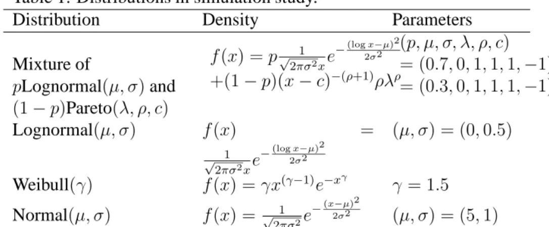
In this work we analyze the same simulated samples as in Buch-Larsen, et al. (2005), which were drawn from four distributions with different tails and different shapes near 0: lognormal, lognormal-Pareto, Weibull and truncated logistic. The distributions and the chosen parameters are listed in Table 1.
Table 1: Distributions in simulation study.
Distribution Density Parameters
Mixture of pLognormal(µ, σ)and (1−p)Pareto(λ, ρ, c) f(x) =p√ 1 2πσ2xe −(logx−µ)2 2σ2 +(1−p)(x−c)−(ρ+1)ρλρ (p, µ, σ, λ, ρ, c) = (0.7,0,1,1,1,−1) = (0.3,0,1,1,1,−1) Lognormal(µ, σ) f(x) = 1 √ 2πσ2xe −(logx−µ)2 2σ2 (µ, σ) = (0,0.5) Weibull(γ) f(x) =γx(γ−1)e−xγ γ = 1.5 Normal(µ, σ) f(x) = √1 2πσ2e −(x−µ)2 2σ2 (µ, σ) = (5,1)
Buch-Larsen, et al. (2005) evaluate the performance of the KMCE tors compared to the estimator described by Clements, et al. (2003), the estima-tor described by Wand, et al. (1991) and the estimaestima-tor described by Bolanc´e, et al. (2003). The Champernowne transformation substantially improve the results from previous authors. Here we see that if the second transformation based on the inverse beta transformation improves the results presented in Buch-Larsen, et al. (2005), this means that the double-transformation method presented here is a substantial gain with respect to existing methods.
We measure the performance of the estimators by the error measures based in L1 norm, L2 norm and W ISE. This last weighs the distance between the estimated and the true distribution with the squared value ofx. This results in an error measure that emphasizes the tail of the distribution, which is very relevant in practice when dealing with income or cost data:
∞ Z 0 b f(x)−f(x)2x2dx 1/2 . (18)
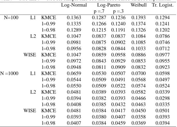
The simulation results can be found in Table 2. For every simulated density and for sample sizes N = 100 and N = 1000, the results presented here cor-respond to the following error measures L1, L2 andW ISE for different values
of the trimming parameter l = 0.99,0.98. The benchmark results are labelled KMCE and they correspond to those presented in Buch-Larsen, et al. (2005).
In general, we can conclude that after a second transformation based on the inverse of a certain Beta distribution cdf the error measures diminish with respect to the KMCE method. In some situations the errors diminish quite substantially with respect to the existing approaches.
We can see that the error measure that shows improvements when using the KIBMCE estimator is theW ISE, which means that this new approach is fitting the tail of positive distributions better than existing alternatives. TheW ISEerror measure is always smaller for the KIBMCE than for the KMCE, at least for one of the two possible value of l that have been used in this simulation study. This would make the KIBMCE estimator specially suitable for positive heavy-tailed distributions. When looking more closely at the results for the mixture of a log-normal distribution and a Pareto tail, we see that larger values ofl are needed to improve the error measures that were encountered with the KMCE method.
We can see that for the Truncated logistic distribution, the lognormal distri-bution and the Weibull distridistri-bution, the method presented here is clearly better than the existing KMCE. We can see in Table 2 that forN = 1000, the KIBMCE
W ISE is about 20% lower than the KMCE W ISE for these distributions. A similar behavior is shown by the other error measures,L1 andL2, forN = 1000, are about 15% lower for the KIBMCE.
Note that the KMCE method was studied in Buch-Larsen, et al. (2005) and the simulation study showed that it improved on the error measures for the existing methodological approaches (Clements, et al., 2003 and Wand, et al., 1991).
Table 2: The estimated error measures for KMCE and KIBMCE
withl= 0.99andl = 0.98for sample size 100 and 1000 based on 2000 repetitions Log-Normal Log-Pareto Weibull Tr. Logist.
p =.7 p =.3 N=100 L1 KMCE 0.1363 0.1287 0.1236 0.1393 0.1294 l=0.99 0.1335 0.1266 0.1240 0.1374 0.1241 l=0.98 0.1289 0.1215 0.1191 0.1326 0.1202 L2 KMCE 0.1047 0.0837 0.0837 0.1084 0.0786 l=0.99 0.0981 0.0875 0.0902 0.1085 0.0746 l=0.98 0.0956 0.0828 0.0844 0.1033 0.0712 WISE KMCE 0.1047 0.0859 0.0958 0.0886 0.0977 l=0.99 0.0972 0.0843 0.0929 0.0853 0.0955 l=0.98 0.0948 0.0811 0.0909 0.0832 0.0923 N =1000 L1 KMCE 0.0659 0.0530 0.0507 0.0700 0.0598 l=0.99 0.0544 0.0509 0.0491 0.0568 0.0497 l=0.98 0.0550 0.0509 0.0522 0.0574 0.0524 L2 KMCE 0.0481 0.0389 0.0393 0.0582 0.0339 l=0.99 0.0394 0.0382 0.0393 0.0466 0.0298 l=0.98 0.0408 0.0385 0.0432 0.0463 0.0335 WISE KMCE 0.0481 0.0384 0.0417 0.0450 0.0501 l=0.99 0.0393 0.0380 0.0407 0.0358 0.0393 l=0.98 0.0407 0.0384 0.0459 0.0369 0.0394
5
Data study
In this section, we apply our estimation method to a data set that contains auto-mobile claim costs from a Spanish insurance company for accidents occurred in 1997. This data set was analyzed in detail by Bolanc´e et al. (2003). It is a typi-cal insurance claims amount data set, i.e. a large sample that looks heavy-tailed. The data are divided into two age groups: claims from policyholders who are less than 30 years old, and claims from policyholders who are 30 years old or older. The first group consists of 1,061 observations in the interval [1;126,000] with mean value 402.70. The second group contains 4,061 observations in the interval [1;17,000] with mean value 243.09. Estimation of the parameters in the modified
Champernowne distribution function for the two samples of is, for young drivers
b
α1 = 1.116, Mc1 = 66,bc1 = 0.000 and for older driversαb2 = 1.145,Mc2 = 68,
b
c2 = 0.000, respectively. We notice that α1 < α2,which indicates that the data set for young drivers has a heavier tail than the data set for older drivers.
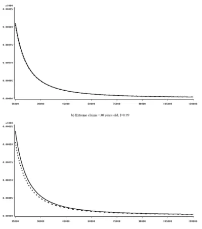
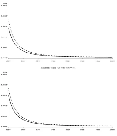
Figure 1 and 2 plot the estimated densities. For small costs, we see that the KIBMCE density in the mode is greater than for the KMCE approach proposed by Buch-Larsen et al. (2005) both for young and older drivers. For both methods, the tail in the estimated density of young policyholders is heavier than the tail of the estimated density of older policyholders. This can be taken as evidence that young drivers are more likely to claim a large amount than older drivers. The KIBMCE method produces lighter tails than the KMCE methods. Based on the results in the simulation study presented in Bolanc´e et al (2008), we believe that the KIBMCE method improves the estimation of the density in the extreme claims class.
Figure 1: KIBMCE withl = 0.99andl= 0.98(solid line) and KMCE (dashed line) estimators of automobile claims
for younger policyholders.
Table 3 presents the V aR(x,0.95) which are obtained from the empirical distribution estimation and those obtained with the KMCE and KIBMCE. We believe that the KIBMCE provides an adequate estimation of the VaR and it seems a recommendable approach to be used in practice.
Table 3: Estimation ofV aR(x,0.95), in thousands. KIBMCE Empirical KMCE l= 0.99 l = 0.98
Young 1104 2912 1601 1716
Figure 2: KIBMCE withl = 0.99andl= 0.98(solid line) and KMCE (dashed line) estimators of automobile claims
for older policyholders.
References
[1] Azzalini, A. (1981): A note on the estimation of a distribution function and quantiles by kernel method. Biometrika, 68, 326-328.
[2] Bolanc´e, C., Guill´en, M. and Nielsen, J.P. (2003): Kernel density estimation of actuarial loss functions. Insurance: Mathematics and Economics, 32, 19-36.
[3] Bolanc´e, C., Guill´en, M. and Nielsen, J.P. (2008): Inverse Beta transforma-tion in kernel density estimatransforma-tion. Statistics & Probability Letters, 78, 1757-1764.
[4] Dutta, K. and Perry, J. (2006): A Tale of Tails: An Empirical Anal-ysis of Loss Distribution Models for Estimating Operational Risk Cap-ital. FRB of Boston Working Paper No. 06-13 Available at SSRN: http://ssrn.com/abstract=918880
[5] Buch-Larsen, T., Guillen, M., Nielsen, J.P. and Bolanc´e, C. (2005): Kernel density estimation for heavy-tailed distributions using the Champernowne transformation. Statistics, 39, 503-518.
[6] Clements, A.E., Hurn, A.S. and Lindsay, K.A. (2003): M¨obius-like map-pings and their use in kernel density estimation. Journal of the American
Statistical Association, 98, 993-1000.
[7] Chavez-Denoulin, V. and Davison, P. (2005): Generalized additive mod-elling of sample extremes. Applied Statistics, 54, 1, 207-222.
[8] Chavez-Denoulin, V. and Embrechts, P. ((2004): Smooth Extremal Models in Finance and Insurance. The Journal of Risk and Insurance, 71, 2, 183-199. [9] Coles, S. (2001): An introduction to statistical modeling of extreme values,
Springer, London.
[10] Cooray, K. and Ananda, M.M.A. (2005): Modeling actuarial data with a composite lognormal-Pareto model. Scandinavian Actuarial Journal, 5, 321-334.
[11] Embrechts, P., Kl¨uppelberg, C. and Mikosch, T. (1999): Modelling Extremal
[12] Jones, M.C. (1990): Variable kernel density estimation and variable kernel density estimation. Australian Journal of Statistics, 32, 361-371.
[13] Reiss, R.D. (1981): Nomparametric estimation of smooth distribution func-tions. Scandinavian Journal Statistics, 8, 116-119.
[14] Reis, R.D. and Thomas M.(2001): Statistical Analysis of Extreme Values:
with Applications to Insurance, Finance, Hydrology and Other Fields, 2nd
Edition. Birkhauser.
[15] Silverman, B.W. (1986): Density Estimation for Statistics and Data
Analy-sis. London: Chapman & Hall.
[16] Swanepoel, J.W. H. and Van Graan F. C. (2005): A new kernel distribution function estimator based on a non-parametric transformation of the data,
Scandinavian Journal of Statistics, 32, 551-562.
[17] Terrell, G.R. (1990): The maximal smoothing principle in density estima-tion. Journal of the American Statistical Association, 85, 270-277.
[18] Terrell, G.R. and Scott, D.W. (1990): Oversmoothed nonparametric density estimates. Journal of the American Statistical Association, 80, 209-214. [19] Wand, M.P. and Jones, M.C. (1995): Kernel Smoothing. London: Chapman
& Hall.
[20] Wand, P., Marron, J.S. and Ruppert, D. (1991): Transformations in density estimation. Journal of the American Statistical Association, 86, 414, 343-361.
[21] Wu, T.-J., Chen, C.-F. and Chen, H.-Y. (2007): A variable bandwidth selec-tor in multivariate kernel density estimation. Statistics & Probability Letters,
Acknowledgement 1 The Spanish Ministry of Education and Science /FEDER