Factor productivity differences and missing trade problems in a regional HOV model

Factor productivity differences and missing trade problems in a regional HOV

model

Andrés Artal-Tur*, Carlos Llano-Verduras**, Francisco Requena-Silvente***

(*) Dpt. of Economics, Technical University of Cartagena, Pº Alfonso XIII, 50, 30203 Cartagena, Spain. (e-mail: [email protected])

(**) Dpt. of Economic Analysis, Autonoma University of Madrid, and CEPREDE, Centro Stone, Lawrence R. Klein Institute, 28049 Cantoblanco, Madrid, Spain.

(e-mail: [email protected])

(***) Dpt. of Applied Economics II, University of Valencia, Avda. Los Naranjos s/n, 46022 Valencia, Spain. (e-mail: [email protected])

Corresponding author: [email protected]

Short running title: “Productivity differences in a regional HOV model”

Abstract

Recent empirical papers testing the performance of the Heckscher-Ohlin-Vanek (HOV) model suggest the need of relaxing its restrictive assumptions in order to reconcile theory and data. This paper wonders if introducing factor productivity differences could help to improve the performance of the HOV model in a regional setting. Using a new dataset of 17 Spanish regions and three different HOV specifications, we seek for the existence of Hicks-neutral (HN) or factor-augmenting industry-neutral (FAIN) technological differences. Data support the existence of HN technological differences, which contributes for a remarkable improvement of the regional HOV performance since the so-called missing trade problem largely disappears.

Keywords: Heckscher-Ohlin-Vanek, Factor Regional Trade, Productivity differences, Missing trade

problem.

JEL classification: F11, F14.

Acknowledgements: The article has benefited from the comments of participants in European Trade Study Group (ETSG) 2008 (Warsaw) and INTECO 2008 (Spain). We would like also thank the suggestions made by James Walker. F. Requena is member of INTECO (GRUPOS03/151). A. Artal and F. Requena acknowledge financial support from the Spanish Ministry of Science and Innovation (project number ECO 2008-04059/ECON).

1. Introduction

The Heckscher-Ohlin (HO) model is a very illustrative example of what a theory should be: simple, rich, ambitious and very insightful. No doubt, this explains its ubiquity in the field of international economics, sometimes used as a framework for studying the location of production, other times for discussing the welfare impact of international trade flows (Bernstein and Weinstein 2002; Davis 1998). Vanek (1968) re-interpreted the model as one of trade in factor services, stating that, under some assumptions1, the model predicts that net export of factor services will be the difference between a region’s endowment and the endowment typical in the world for a region of that size. The importance of his contribution was establishing a testable relationship between factor endowments, factor input requirements and (net) factor trade, the so-called Heckscher-Ohlin-Vanek (HOV) equation.

This contribution obviously stimulated academic curiosity in order to see how the model performed empirically, with early tests showing a poor predictive power of the HOV model using a large number of countries and factors (Maskus 1985; Bowen et al. 1987). As a response, more recent contributions have followed the path of relaxing some of the strict assumptions of the original model, extending it in a way more consistent with observed data. In the country approach, these contributions have shown the prominent role that the assumptions of international identical technologies, factor price equalization, and identical and homothetic preferences play in reconciling theory and evidence (Trefler 1995; Davis and Weinstein 2001).2

Interregional trade flow data rather than international trade data can alternatively be used to test the performance of the HOV model. A priori, regional tests of the basic HOV model are expected to

1 _{The strict version assumes: (1) identical constant returns to scale (CRS) technology; (2) perfectly competitive markets in} goods and factors; (3) identical and homothetic preferences; (4) factor endowment are different (but not too different) across countries; and (5) free trade in goods.

2 _{Under the assumption of universal factor price equalization, endowments can be measured in physical units (i.e. number of} employees) rather than in currency (i.e. labour compensation) because factor prices are the same across countries.

show a superior performance, because the three key assumptions of the model - identical technologies, factor price equalization and identical and homothetic demands – are more plausible to hold in a regional setting than in an international one. The pioneer contribution of Davis et al. (1997), using data on the prefectures of Japan, found that relaxing the world factor price equalisation assumption, but maintaining it for Japan, was enough to obtain a remarkable improvement of the match between theory and data.3 In contrast, Artal et al. (2006) and Requena et al. (2008a), using data on 14 Spanish regions, found a remarkable performance of the strict HOV model when predicting the direction of factor trade services,

but serious missing trade problems remain when predicting the volume of factor trade services; their

results show that the theoretical model predicts much more factor trade than the one we observe in data. In this paper we get deeper understanding of how well the HOV model works, paying especial attention to whether technology differences between trading partners help improve the performance of the HOV model in a regional setting.4 Our approach assumes that regions could present differences in their unit factor requirements, but arraying solely from the existence of differences in their factor productivities. It allows us still assuming that regions share identical production technologies once we account for productivity differences. With this aim, we address two specifications of technological differences: Hicks-neutral (HN) and factor-augmenting industry-neutral (FAIN). In the HN specification, productivity differs among regions uniformly for all factors, but it is the same (“neutral”) across industries; in the FAIN specification, productivity is different for each region-factor pair but such differences remain constant across industries.

3 _{In practice Davis et al (1997) used the Japanese Input-Output Table rather than the replaced the US Input-Output Table in} the calculation of the measured factor content of trade of the Japanese prefectures to show that there are important differences in technology across countries.

4 _{Davis et al (1997) did not address this question because they had only the Japanese Input-Output Table. Requena et al.} (2008a) investigated the importance of Hicks-neutral technological differences across Spanish regions by simply scaling factor endowments by per capita GDP differences as suggested in Trefler (1993). The results showed that such a simple

Our analysis will focus on the Spanish interregional trade flows, which accounts for 80% of total Spanish trade. Requena et al. (2008b) show that the uneven distribution of production factors that induces intranational specialisation and different regional factor prices is not an issue for Spain. Since factor endowments differences are not too large across Spanish regions (i.e. national FPE holds), intranational space becomes a good setting to investigate the impact of technology differences on the factor trade model.

A first novelty of the paper is to apply three different specifications in testing the performance of the HOV model: the standard model, the pair-wise model, and the relative model. The first one is the most commonly used in the literature to evaluate the HOV model and it is based on a region by region comparison for each factor. The second one follows Hakura (2001) and it is based on comparisons between all pairs of regions for each factor. The third one follows Debaere (2003) and it is based on comparisons of factor contents and factor abundances between pairs of regions for each pair of factors. The pair-wise model and the relative model have two advantages regarding the standard model. First, bilateral comparisons increase the number of observations employed in the tests, improving the robustness of the results. Second, although less important in a regional framework, is the fact that comparisons between regions do not require a vector of world or national endowments.5

A second novelty of the paper is the use of a new database of Spanish Input-Output regional tables (Llano, 2004a, 2004b; Pérez et al, 2008). This newly constructed data set provides homogeneous information on trade flows, gross production, absorption patterns and technical coefficients for 17 Spanish regions, notably improving the data set characteristics, and allowing us to eliminate common measurement errors (Davis and Weinstein 2001). The new database expands the scope of previous exercises incorporating information not before available for three Spanish regions (Murcia, Cantabria

and La Rioja). Moreover, all data used in the estimation of regional technology parameters in the empirical exercise is now provided by a unique source, the Lawrence-Klein Institute at the Autonoma University of Madrid, who developed an intense statistical effort of data homogenisation when building the whole regional Input-Output framework.6 Gains in quality of data are of salient relevance, given that previous data sets were surveyed separately by 14 different regional statistical agencies (see, Artal et al. 2006).7

Our results provide evidence on the importance of accounting for technological differences in a regional HOV framework. First, the capacity to predict the direction of factor trade services improves compared to the benchmark HOV model that assumes no productivity differences across regions. Second, and more interestingly, the missing trade problem largely disappears. This novel result indicates that regional productivity differences are the main reason why the HOV model was not accurately predicting the observed volume of factor services across Spanish regions. The HN specification seems to work slightly better in the regional HOV case, although the FAIN specification follows very closely.

After this introduction, the remainder of the paper is organised as follows. Section 2 defines three different methods employed in testing the extended version of the model. Section 3 describes the econometric specification in order to estimate productivity differences among the Spanish regions. Section 4 includes the data set and discusses the results of the research, while section 5 states the conclusions of the paper.

2. Three HOV specifications copying with productivity differences

In this section we present the HOV model and introduce efficiency adjustments in the use of the production factors across regions in a manner compatible with the fact that all regions use the same input 5 _{This property of the bilateral comparisons is more important when using international data due to the difficulty of computing} a vector of “world” endowments and the subsequent problems of statistical homogeneity (see Debaere 2003).

requirements measured in efficiency units in each industry. Our model builds on three different approaches to the HOV equation: the standard, the pair-wise and the relative versions. First we present the basic specification of each HOV equation and then extend it to its productivity-adjusted specification, which will be further employed in testing the modified model’s performance.

2.1 The standard HOV model

Let r, i, and f index regions, industries, and factors, respectively, with country S (for Spain)

having R regions, I industries, and F primary factors. Let Tr =Er −Mr be the interregional net trade

vector for region r, constructed as the difference between the export and import vectors for region r, and 1

S(I B )

D − _S − be country’s S technology matrix that transforms good flows into their total (direct and indirect) embodied factor services. The elements of matrix Dare defined as ratios between domestic

factor endowment by industry by the corresponding output. The elements of matrix Bare defined as ratios between domestic usage of each input and industry output.8 The observed factor content in region r

expresses the quantity of factor embodied in the net exports of region r and is obtained from multiplying

the Spanish technology matrix times the vector of net exports of region r , D_S(I−B_S)−1T_r. If a_S´f is a

vector of the technological matrix, the measured content of trade in factor f in region r is f _r S f S a T F = ´ . Let f r

V and VSf be the endowment of factor f in region r and country S, respectively; Yr be the gross national product (GNP) of region r, Y_S be country’s S GNP, and N_r be the trade balance of region

7 _{In addition, we use a new measure of the stock of physical capital provided by Fundación BBVA (2006).}

8 _{Each element (} fi) of matrix D_S(I−B_S)−1 is = +

∑

a , that is, the direct factor input plus the sum for each industry j of the indirect factor input, where the latter takes into account all intermediated inputs to industry i. Notice that

the direct input matrix and the input-output matrices for each region also include only the usage of domestically produced intermediates.

r, so that s_r =(Y_r −N_r)/Y_S captures the final consumption shares of region r in the national space.9 In

this framework, the standard regional HOV model shows that, under standard assumptions, the predicted factor content of trade for factor f in region r is equal to the difference between the region’s factor

endowments ( f r

V ) and the national endowments (

∑

) adjusted by the final consumption share of region r in the country (sr). If the theory is correct, the HOV equation can be written as:

∑

where the left hand side expression is the measured factor content of trade and the right hand side is the predicted factor content of trade.

Departing from the standard model by introducing regional factor-productivity differences requires the use of a technology parameter, f

r

π , such that if f r

V is the factor endowment of f in region r,

then f r f r f r V

V* =π would be the corresponding factor endowment measured in productivity-equivalent

units.10 We assume identical technologies at the productivity-equivalent level and normalize factor productivity of country S to be equal to one: π_rfA (I - B )_{r r} -1 =A (I - B )_{S S} -1, r =1…R, with π_rf being the productivity of region r relative to country S for factor f.11 Then equation (2) provides a specification for

the productivity-adjusted standard HOV model, with the right hand side of the expression capturing the excess of region’s r endowments supply in efficiency terms:

∑

Notice that the expression in left hand side (the measured factor content of trade) has not changed.

9 _{Since regions are open-economies, their trade balances represent a higher percentage of their GDP compared to Spanish’s} trade balance.

10 _{We assume that all differences in technology across regions arise in the form of factor-augmenting productivity differences} (HN or FAIN), following Trefler (1993)’s insight.

2.2 The pair-wise HOV model

In order to obtain the pair-wise HOV model (Staiger et al. 1987; Hakura 2001), we adopt a two-region version of the strict Vanek equation (1) for two given two-regions 1 and 2, and factor f:12

f f f f V V F F₁ −α ₂ = ₁ −α ₂ (3)

where α =s₁/s₂, F₁f −αF₂f is the measured pair-wise factor content of trade

(F₁ =D₁(I−B₁)−1T₁andF₂ =D₂(I−B₂)−1T₂), and V₁f −αV₂f is the predicted pair-wise factor content

of trade.13

This version requires all assumptions of the basic HOV model to hold. Further, we can relax the assumption of identical regional technology, withA (I - B )_{r r} -1≠A (I - B )_{r´ r´} -1≠A (I - B )_{S S} -1,∀ ≠r r´, obtaining in this way the version popularised by Staiger et al. (1987) and more recently used by Hakura (2001). In order to specify the model in its productivity-equivalent version, we start defining a vector of technology parameters of the form f_´

rr

π that captures the productivity ratio by pairs of regions in country

S. Given that productivity differences are the unique technology differences allowed for in the model,

regions will share the same technology matrix at the productivity-equivalent level for every factor f, that

is, f_´ rr π = -1 -1 r r r´ r´

A (I - B ) (I - B ) A , with FPE holding at a national level (Trefler 1993, 1995).

11 _{We normalize respect to the country technology by convenience, but one could have normalized respect to a region of} reference as it is usual in the country approaches (see, for example, Trefler 1993, 1995).

12 _Defining

∑

∑

∑

and reordering terms, we obtain equation (3).

13 _{Note that in the strict pair-wise regional version we assume identical technologies at the national level, with} ,∀r

-1 -1

r r S S

Introducing productivity differences for two given regions 1 and 2, leads to the following specification of the model14:

f f f f f V V F F₁ −α ₂ =π_{21 1} −α ₂ (4)

with equation (4) expressing the pair-wise HOV equation in productivity-equivalent units, in terms of region 2’s technology.

2.3 The relative HOV model

The relative version of the Vanek equation was proposed by Debaere (2003) as an extension of the basic HOV model, and it is based on comparisons of endowments and observed factor trade services by pairs of factors and regions. In order to obtain the simple version of the relative HOV model, we start with the strict Vanek equation for a region r and a factor f, under standard assumptions, as displayed in

(1). Dividing both sides of equation (1) by the regional consumption share (sr), and defining

r f r f r F s f = and v_rf = V_rf s_r yields,

∑

. Extending this expression for two given regions r and r´, taking the difference between them, and dividing both sides of the resulting equation by

the sum of both region’s normalised endowments, f

r f r v v + _´, we obtain

(

) (

) (

) (

)

14 _{Derivation of the pair-wise HOV model with factor-productivity adjustments assumes that}

12 f π = -1 -1 1 1 2 2 A (I - B ) A (I - B ) . Applying it for region 1 and factor f, we have two equations: (1) π₁₂A (I - B ) T_{2 2} -1 ₁= −V₁ π₁₂A (I - B ) C_{2 2} -1 ₁ and

(2) -1 = −V₂ -1

2 2 2 2 2 2

A (I-B ) T A (I-B ) C. Pre-multiplying (1) with π₁₂−1=π₂₁=A (I -B )_{2 2} -1 A (I -B )_{1 1} -1and (2) with α, taking the

difference between the two equations, and noting that in the pair-wise version C₁ =αC₂ (Staiger et al. 1987; Brecher and Choudri 1988), we obtain equation (4).

Now, if we compute this expression for a supplementary factor f´ and again take differences, we

obtain the basic version of the relative HOV equation. Debaere’s proposal provides a testable modified version of the standard HOV model that compares standardized relative factor contents of trade and endowments by pairs of factors between regions:

´ ´ ´ ´ ´ ´ ´ ´ ´ ´ ´ ´ ´ ´ ´ ´ f r f r f r f r f r f r f r f r f r f r f r f r f r f r f r f r v v v v v v v v v v f f v v f f + − − + − = + − − + − (5)

Introducing regional productivity differences in the relative HOV model requires premultiplying every region’s factor endowment by its productivity measure f

r

π in equation (5). In order to make it simpler, we again normalize factor productivity of country S to unity ( f

r π -1= -1 r r S S A (I - B ) A (I - B ) , r =1—R), with f r

π being the productivity of region r relative to country S, for factor f. Then, we define

factor endowments at the productivity-equivalent level as f r f r r f r f r r f r f r V s V s v v* = * =π =π , with the

productivity-adjusted relative model yielding:

´ ´ * ´ * ´ ´ * ´ * ´ * * ´ * * ´ ´ * ´ * ´ ´ ´ ´ * * ´ f r f r f r f r f r f r f r f r f r f r f r f r f r f r f r f r v v v v v v v v v v f f v v f f + − − + − = + − − + − (6) and f f / / r r r r r r f =π A (I - A ) T_{r r} -1 s =A (I - B ) T_{S S} -1 s for factor f.

3. Estimating regional factor productivity differences

We have just defined the theoretical framework of the investigation, both in the basic specification and in the productivity-adjusted extension. In this section, we estimate the factor-augmenting parameters of the three versions of the HOV model, further incorporating them in the extended models in order to see how these new specifications affect the performance of the model, with a primary focus on missing trade questions.

In the basic versions of every HOV model, standard, pair-wise or relative, we assume the existence of identical technologies in a national-FPE framework, with all regions of country S having the

same technology matrix ( -1 -1

r r S S

A (I - B ) = A (I - B ) ), and consequently every regional industry i

presenting the same unit total (direct and indirect) factor requirement for every factor f (a a rfi r

fi

S = ´ ,∀

´ ).

Within the new framework, once we allow for regional technological differences in the form of factor efficiency gaps, regions will continue to share identical production technologies but now at the productivity-equivalent level, observing the equality of adjusted total unit factor requirements:

fi r fi * S a´ a´ = , with fi r f r fi r a´ a´* _{=π and} f r

π representing productivity of factor f in region r relative to

country S.

Following this approach, we estimate two types of factor-augmenting technological differences by regressing unit total factor requirements of country S (Spain) against those of region r. In the first

specification we allow for factor-augmenting productivities common to every factor f in region r and

industry i, that is, in a HN fashion (π_rf =π_r,∀f ):

i r i r r i=π _a´ +ε a´_S (7)

In the second specification of the technological parameters, we allow for the existence of regional productivity differences specific to every factor, in a factor-augmenting industry-neutral specification (π_rf ≠π_r,∀f ), and estimate the following equation:

fi r fi r f r fi=π _a´ +ε a´_S (8)

Equations (7) and (8) allows for regional technological differences arising in the form of productivity differences. Both equations are estimated using data that vary across 20 industries for each of the 17 regions through seemingly unrelated equations regressions (SURE), what ensures that the

estimation of productivity parameters is not only consistent but also efficient. This procedure is used for the standard and relative versions of the HOV model. In estimating productivity parameters in the pair-wise version of the model, we apply the next specification for every regional pair:

i 1 i 1 21 i 2 a´ a´ =π +ε (9) fi fi f fi 1 1 21 2 a´ a´ =π +ε (10)

where π₂₁ is the productivity of region 2 in terms of region 1, uniform for all factors in equation (9) or factor-specific in equation (10). Both equations allows us estimating interregional productivity differences, now for all binary combination of regions rather than simply for each region relative to Spain, the country of reference. In all cases, we assume that factor requirements are generated by a process obeying to the HN or FAIN assumptions, with measurement errors randomly distributed around zero and embodied in the residual terms.15

After equations (7)-(10) have been estimated, we incorporate the productivity estimates in the extended versions of the HOV model [either equation (2), (4) or (6)], and then explore how it affects the performance of the model through the standard tests of sign, variance ratios and slope of the regressions of actual versus predicted factor contents of trade for the Spanish regions.16

4. Data and results

4.1 Data

The research is based primarily on information coming from a set of homogeneous input-output (IO) tables for 17 Spanish regions, developed by the Lawrence-Klein Institute at the Autonoma University of Madrid with the aim of estimating the first Spanish inter-regional Input-Output model. The

15 _{This procedure permits the model staying at the productivity-equivalent framework, avoiding at the same time the criticism} by Gabaix (1997) to the original Trefler’s (1993) approach, which was previously implemented in Requena et al (2008a).

importance of this newly constructed data set is that it provides comparable data on trade flows, gross production, absorption patterns and technical coefficients for all of the Spanish regions in the year 1995, significantly improving available information to date, which only could be obtained by the compilation of information provided -for different years and dissimilar methodologies- by 14 different regional statistical offices, with all the heterogeneity it introduces in the model. This new data set also allows us to incorporate three new Spanish regions to the study, La Rioja, Murcia and Cantabria, regions for whom there were not available information to date. The regional data set is equally compatible with the country or national statistical framework, with aggregated regional information coherently reproducing the national accounting system, what markedly improves previous data set characteristics, and it is important in terms of efficiently capturing the production and absorption (consumption plus investment) patterns present in the HOV framework. In this way, the homogeneity of regional IO data allows us to compute comparable technical coefficients for every Spanish region, what then will be used to estimate our productivity parameters.

Additionally, we will use the input-output table of Spain in 1995 when computing the factor content of trade for the strict and extended versions of the regional HOV model, and, through the use of its technical coefficients, it will provide the technology of reference when estimating our regional specific productivity estimates. Direct input requirements are constructed as factor endowments divided by gross output, while total input requirements imply multiplying direct requirement vectors by corresponding Leontief inverse tables. Trade flows come from the Input-Output tables, which allow us to breakdown the trade vectors of every Spanish region in their interregional and international flows.

We use three production factors: physical capital (K), high educated labour (H), low educated labour (L). Endowment data is taken from Encuesta de Población Activa and from National Accounts

16 _{The tests employed in the paper are standards in the HOV literature. We describe them in more detail in the following}

(INE-National Statistics Institute; www.ine.es) for the labour force, which classifies the labour force regional vectors in terms of education levels, with high educated individuals defined as those with secondary and above levels of enrolment and low educated ones as those that have not finished the secondary studies or have a lower level of education. Data on physical capital stock comes from the new database launched by Fundación BBVA, which applies a methodological revision to its precedent work

in El stock y los servicios del capital en España y su distribución territorial (1964-2005). Nueva

metodología, following new methodological recommendations of the OECD (see, www.fbbva.es, for

further details).17

Our database then compiles a new data set of 20-industries, including primary, secondary and tertiary activities, for 17 Spanish regions plus the country as a whole, and for 3 production factors (K, H and L). More details on the data composition can be found in the Appendix.

4.2 Results

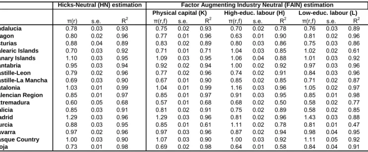
Table 1 presents the results of estimating productivity parameters for the regions of Spain. We include two types of results: in the first data column of the table we report the productivity estimates of Spanish regions relative to those of Spain as a whole for every factor in the HN specification (π_r) (equation 7). The following three columns of the table include the same information for the FAIN specification ( f

r

π ) (equation 8). We do not report a table containing the estimated pair-wise productivity

subsection.

17 _{Out of the three new measures of capital stock proposed by Fundación BBVA (gross, net and productive), we choose gross} capital stock as it is the one more closely related to the concept of “endowment”.

parameters because of the great number of results it supposes: for each factor under the HN specification we estimate 272 parameters (=17*16).18

Productivity estimates of the regions of Spain in the HN assumption show that Madrid is the most productive region; the value of 1.29 means that Madrid uses 29 percent less of each factor to produce one final unit of output in all industries than Spain as a whole does. It is followed by Canary Islands (1.10), Catalonia (1.03) and Basque country (1.00). The least productive regions in Spain appear to be Extremadura (0.60), Castille-La Mancha (0.69) and Andalusia (0.78). The degree of dispersion in the value of coefficients ranging from 0.60 to 1.29 reveals the existence of substantial regional productivity differences, and therefore, of efficiency-based factor endowments differences across regions. In addition the degree of adjustment shows a remarkable achievement of the estimation by SURE procedure. All regions exhibit a 2

R statistic equal to or greater than 0.9 except for Extremadura (0.68) and Asturias

(0.89).

In terms of individual factors, now under the FAIN assumption, we observe clear differences with respect to the HN estimates in all three factors of production. For example, in the case of Madrid, efficiency gains in terms of capital unit requirements in the FAIN specification coincide in value (1.29) with those obtained for the three factors jointly in the HN specification. However, the FAIN specification reveals that Madrid is less efficient than other regions in the use of high-educated labour (up to 19 percent inferior) while it is highly efficient in the use of low-educated labour across industries (up to 43 percent more than the entire country). In general, the coefficients obtained for the physical capital in the FAIN specification appear to be closer to those obtained in the HN specification, while bigger differences seem to emerge for the two types of labour. For example, in the case of low-educated labour factor (L), some regions (Murcia, Valencian Region, Castille-La Mancha, Catalonia and Balearic

Islands) experience important productivity gains in comparison with their HN estimates and others regions (Navarra, Madrid, La Rioja and Aragon) lose positions in the national ranking.

When we tested whether the FAIN coefficients for the three factor were the same as the one obtained from the HN specification, in all cases the null hypothesis of equality was rejected at conventional significance levels. Therefore, and a priori, the FAIN specification is preferred to the HN specification from an econometric point of view.

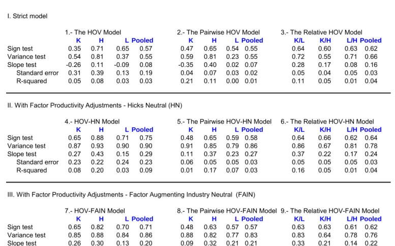
After computing regional technological parameters, we apply our productivity estimates to the three versions of the HOV model in order to check how technological assumption affects its performance in a regional setting. We run three commonly used tests in testing the performance of the HOV model: the sign test, the variance ratio and the slope test. The three tests compare both sides of the model´s equation: the actual vs the predicted factor contents of trade. The sign test counts the number of signs that match in both sides of the equation. Therefore the test examines whether the direction of the actual factor content of trade coincides with the direction that the model predicts. The variance ratio compares the variance of both the actual and the predicted factor content of trade. The larger the variance ratio, the more volume of the factor content of net exports is explained by the model. A variance ratio far below one means that the amount of factor trade predicted by the model is much larger than the amount of actual (observed) factor trade: the so-called “missing trade problem”. The coefficient of the slope test is the result of the regression of the normalised value of the actual factor content of trade against the predicted factor content of trade. As in the other two tests, the slope coefficient should be equal to one in order to achieve a “perfect performance” of the HOV model (Trefler 1995).19

Table 2 presents the results for the three versions of the HOV model (standard, pair-wise and relative), with every column containing the results for the basic and extended models (HN and FAIN).

The standard HOV model (first column of first panel), shows a limited predictive capacity in its strict version for pooled factors, with a sign value of 0.57 (0.35 for K, 0.71 for H and 0.65 for L, individually), a variance test value of 0.55 (0.54 for K, 0.81 for H and 0.37 for L) and the slope test reports a coefficient of 0.08 which is not statistically significant. In addition the slope coefficients for K and L exhibit negative values.

Extending the standard HOV equation to accommodate HN technology differences (first column of second panel), clearly improves the performance of the model, reaching values for pooled factors of 0.75 in the sign test (0.65 for K, 0.88 for H and 0.71 for L) and showing a positive value for the three individual coefficients in the slope tests (0.29 for pooled factors), although they remain not statistically significant. Moreover, introducing the HN assumption for the standard HOV equation clearly makes the missing trade problem nearly disappearing, pushing the variance ratio to a value of 0.90 for pooled factors (0.87 for K, 0.93 for H and 0.90 for L).

Introducing the FAIN technology assumption in the standard model (first column of third panel) also provides a remarkable improvement of the Vanek equation performance, with pooled factors showing slightly below values in all tests in comparison with the HN extension: 0.71 in the sign test, 0.86 in the variance ratio and 0.20 in the slope test. In this way, it seems that for the Vanek equation version, extending the HOV model through the introduction of measurement of factors in efficiency terms clearly improves its performance, not just pushing up its predictive capacity in terms of direction and volume of trade, but also making the missing trade problem almost disappearing.

Moving to the results for the pair-wise version of the HOV model (second column of first panel), we observe that the strict pair-wise specification reports similar results than those of the standard HOV 19 _{Note than in the slope test we are not just measuring how the model predicts the volume of factor trade services, but the}

model. It performs badly in terms of sign, variance ratio and slope test, with values of 0.55, 0.55 and 0.07 for pooled factors, respectively. Extending the pair-wise HOV model by introducing HN technology adjustments (second column of second panel) improves the performance of the model particularly in terms of the variance ratio, nearly solving the missing trade problem for physical capital (with a variance ratio of 0.91) and remarkably reducing missing trade for the other two factors, with test values of 0.85 for H and 0.79 for L. Slope test values improve again for K and L, with the pooled factor value shifting from 0.07 in the basic pair-wise version to 0.27 in the pair-wise HN extension, with all estimated coefficients now being statistically significants. The FAIN extension of the pair-wise HOV model reflects an improvement in the model’s performance of approximately the same magnitude than that of the HN case, although all values systematically are slightly lower than those of the HN case.

Finally, in the relative HOV model case, we observe that the strict version (column 3 of first panel) performs a little bit better than the Standard and the Pair-wise strict versions, with test values reaching 0.62, 0.66 and 0.16, for the sign, the variance ratio and the slope tests, respectively. Although being conscious that these test values still reflect a poor performance of the relative HOV model in its strict version, it is interesting to note that the slope test values for factor pairs (K/L, K/H and L/H) depart from more rationale values (0.28 for K/L and 0.17 for K/H) than in the other two basic versions of the model, while the missing trade problem is of much less importance in this basic relative HOV specification (0.72 for K/L and 0.71 for L/H), what seems to reflect some of the advantages that the relative model presents in comparison with the other two specifications. Once we introduce the HN extension in the relative HOV model (column 3 of second panel), we observe an improvement in the model’s performance in terms of missing trade and slope test values, but not a remarkable improvement in the capacity of the model to predict the factor trade direction, with sign test values remaining

relatively stable. The FAIN extension (column 3 of third panel) yields similar results, with the variance ratio and the slope test showing values that are just a bit smaller than those found in the HN case.

Our results point out that, in general, a better measurement of endowments in efficiency terms allows for an improvement of the model’s performance in a regional HOV framework, markedly reducing the missing trade problem. In terms of predicting the direction of trade, introducing technological differences in the HOV model also improves the predictive capacity of the HOV model, but there are differences in the size of the improvement: it is large for the standard version but not so much for the pair-wise and relative HOV versions. We also observe that correcting for productivity differences raises the value of the coefficient of the slope test and made the coefficients statistically significant in all three versions. Finally, the performance of the standard HOV specification is more sensitive to the introduction of endowment measures in efficiency terms compared to the pair-wise and the relative versions.

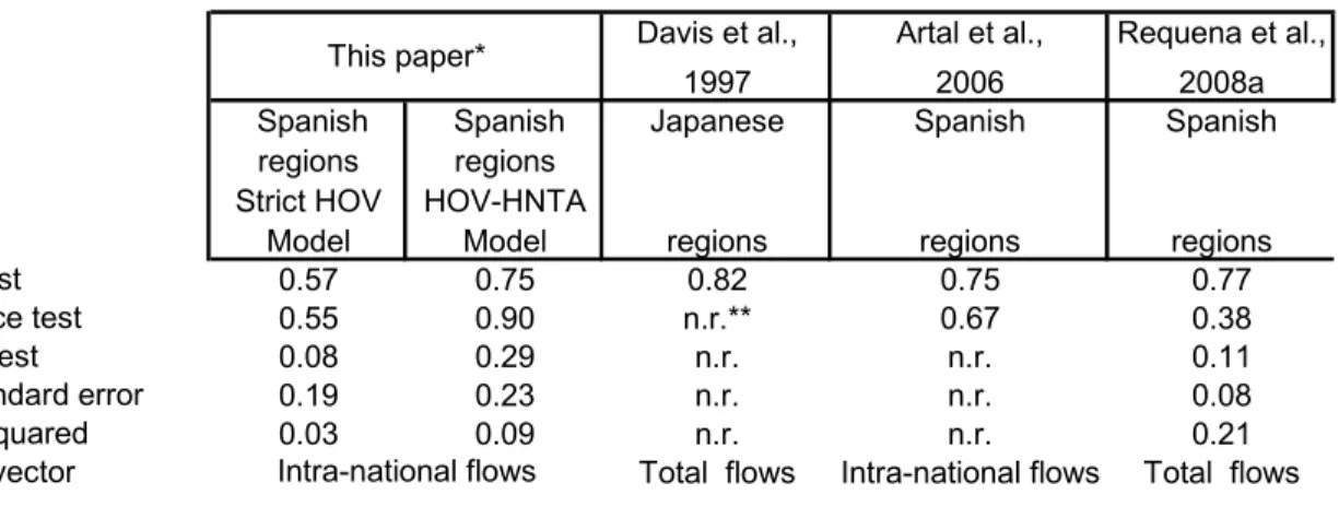
We conclude our analysis by providing a comparison of our results with those found previously in the empirical literature. So far, there are other three papers that have analysed the HOV model using intra-national trade flows. Davis et al (1997) for Japan prefectures did not have regional IO tables so trade was estimated as the difference between production and consumption. Since they have only the IO table of Japan, they could not investigate the role of technological differences. Artal et al (2006) and Requena et al (2008a) used 14 Spanish regional IO tables, which were not perfectly comparable, so they did not attempt to estimate technological differences across regions. By contrast, our paper employs a new and homogeneous data set for 17 Spanish regions, making it appropriate to estimate productivity gaps between regions. Alike us, Davis et al (1997) used three production factors (K,L,H), Artal et al. (2006) used an additional land factor and Requena et al. (2008a) did it for arable land and pasture, woodland and R&D capital. Another difference between those papers is the vector of trade employed.

Davis et al (1997) and Requena et al (2008a) use total (intra and international) trade flows, while Artal et al (2006) and our paper use only intra-national trade flows.

Table 3 compares the results of the four papers mentioned above. The direction-of-trade test (sign test) display similar results across the different papers. The coefficient of the slope test remains far from 1 across all the papers. The most notable improvement occurs in the variance ratio after introducing HN technological differences in the HOV model, moving from a test value of 0.55 to another of 0.90.

5. Conclusions

The strict version of HOV model has been repeatedly rejected empirically using international data. Relaxing identical technology and FPE assumptions at a universal level has been mandatory in order to achieve a good performance of the HOV model using country-level data. In this paper we explore whether the introduction of technological differences at a regional level (in a setting where FPE holds) may help to improve the performance of the HOV model, particularly investigating its effects on the important missing trade problem found in previous exercises.

With this aim, we estimate factor-productivity parameters from each region’s actual technologies, and address two specifications of technological differences: Hicks-neutral (HN) and factor-augmenting industry-neutral (FAIN). Then, we extend the model allowing for factor productivity-adjusted versions and test how these changes affect the model’s performance for three different HOV specifications: the standard model, the pair-wise model, and the relative model.

Using a new data set for 17 Spanish regions, we find evidence supporting the assumption of HN technological differences, with all test values improving markedly in the standard HOV equation case. The pair-wise and the relative versions of the model equally show how the missing trade problem almost disappears once we account for this kind of model extension. In this context, our results indicate that accounting for productivity differences is also an appropriate modification of HOV models at a regional

scale, as it has been shown in the country exercises, although HN is revealed as slightly more adequate in capturing regional technological differences than the FAIN assumption.

The contribution here is to show that a simpler technical modification can establish considerable gains in the predictive performance of the HOV model, nearly solving the missing trade problem, with FPE still holding at a national scale. Therefore, improving the measurement of endowments is showed as a primary way of reducing the missing trade problems in a regional HOV framework, a result that contributes to improve previous findings of the regional HOV literature.

References

Artal A, Castillo J, Requena F (2006) Contrastación empírica del modelo de dotaciones factoriales para el comercio interregional de España. Investigaciones Económicas 30: 283-316

Bernstein J R, Weinstein D E (2002) Do Endowments Predict the Location of Production? Evidence from National and International Data. Journal of International Economics 56: 55-76

Bowen H P, Leamer E, Sveikauskas L (1987) Multicountry, Multifactor Tests of the Factor Abundance Theory. American Economic Review 77 (5): 791-809

Brecher R A, Choudri E U (1988) The factor content of consumption in Canada and the United States: A two country test of the Heckscher-Ohlin-Vanek model.In: Feenstra R.C. (ed) Empirical Methods for

International Trade. MIT Press, Cambridge

Davis D R (1998) Does European Unemployment Prop up American Wages? National Labor Markets and Global Trade. American Economic Review 88 (3): 478-494

Davis D R, Weinstein DE, Bradford SC, Shimpo K (1997) Using International and Japanese Regional Data to Determine When the Factor Abundance Theory of Trade Works. American Economic

Review 87: 421-46

Davis D R, Weinstein D E (2001) An Account of Global Factor Trade. American Economic Review 91

(5): 1423-1453

Debaere P (2003) Relative Factor Abundance and Trade. Journal of Political Economy 111 (3): 589-610

Gabaix X (1997) The Factor Content of Trade: A Rejection of the Heckscher-Ohlin-Leontief Hypothesis. Harvard University, mimeo

Hakura D (2001) Why does HOV fail? The role of technological differences within the EC. Journal of

International Economics 54: 361-382

Llano C (2004a) Economía sectorial y espacial: el comercio interregional en el marco input-output. Instituto de Estudios Fiscales. Colección Investigaciones 1

Llano C (2004b) The Interregional Trade in the Context of a Multirregional Input-Output Model for Spain. Estudios de Economía Aplicada 22: 1-34

Maskus K E (1985) A test of the Heckscher-Ohlin-Vanek Theorem: The Leontief commonplace. Journal

of International Economics 19 (3-4): 201-212

Maskus K E, Nishioka S (2009) Development-Related Biases in Factor Productivities and the HOV Model of Trade, Canadian Journal of Economics, forthcoming

Pérez J, Dones M, Llano C (2008) An Interregional impact analysis of the EU Spanish Structural Funds in Spain (1995-1999). Papers in Regional Science, forthcoming

Requena F, Artal A, Castillo J (2008a) Testing Heckscher-Ohlin-Vanek model using Spanish regional data. International Regional Science Review 31 (2): 159-184

Requena F, Castillo J, Artal A (2008b) Is Spain a lumpy country? A dynamic analysis of the “lens condition”. Applied Economic Letters 15 (3): 175-180

Staiger R M, Deardorff A V, Stern R M (1987) An Evaluation of Factor Endowments and Protection as Determinants of Japanese and American Foreign Trade. Canadian Journal of Economics 20:

449-463

Trefler D (1993) International Factor Price Differences: Leontief was Right!. Journal of Political

Economy 101: 961-987

Trefler D (1995) The Case of Missing Trade and Other Mysteries. American Economic Review 85 (5):

1029-1046

Vanek J (1968) The factor proportions theory: the n-factor case. Kyklos 4: 749-756

Van der Linden J A, and Oosterhaven J (1995) Intercountry EC input-output relations: construction method and main results for 1965-1985. Economic System Research, 7 (3): 249 – 269

APPENDIX

A) Technical Appendix

As Debaere (2003) demonstrated, equation (5) is directly related to relative factor abundance as showed in equation (A1):

⎟⎟ ⎠ ⎞ ⎜⎜ ⎝ ⎛ + + − + = + − − + − f r f r f r f r f r f r f r f r f r f r f r f r f r f r f r f r f r v v v v v v v v v v v f f v v f f ´ ´ ´ ´ ´ ´ ´ ´ ´ ´ ´ ´ ´ ´ ´ ´ ´ ´ ´ 2 _(A1)

For any two factors f and f´, a region r is said to be relatively abundant in factor f compared to

region r´ always that v_rf v_rf´ >v_rf_´ v_rf_´´ . Debaere (2003) showed that this statement holds if and only if

(

) (

)

v_´´ _´ > ´ + _´´ + _´ , which determines the sign of the right-hand side of equation (A1). It

establishes a direct relationship between relative factor abundance and the right-hand side of equation (5), what leads this equation to be named as the relative abundance equation.

Rewriting relative factor abundance as:

´ ´ * ´ ´ ´ * ´ * ´ * ´ ´ ´ * ´ ´ ´ * ´ * ´ * ´ ´ ´ ´ * ´ ´ * ´ ´ * * ´ ´ ´ ´ / / / / f r f r f r f r f r f r f r f r f r f r f r f r f r f r f r f r f r f r f r f r f r f r f r f r f r f r f r f r v v v v v v v v v v v v v v v v π π π π π π π π π π π π > ⇔ > ⇔ > = > (A2)

we obtain that in the factor-augmenting case, the relative factor abundance ratio without productivity adjustments ( _/ f´

r f r v

v or v_rf_´/v_rf_´´) is the product of the productivity-equivalent relative factor abundance

ratio ( * _/ *f´ r f r v v or * ´/ *´´ f r f r v

v ) and the factor-productivity ratio (π_rf_´/π_rf or π_rf_´´/π_rf´). In the Hicks-neutral

(HN) case, factor-productivity ratios remain the same for every factor f or f´ and every pair of regions r

with or without productivity adjustments (Debaere, 2003, p. 609). Nevertheless, in the factor-augmenting industry-neutral (FAIN) case, where productivities of factors could differ inside a region

( ´ ´ ´ ´/ / f r f r f r f r π π π

π ≠ ), the relative factor abundance definition differs from the basic specification (Maskus and Nishioka, 2009): ´ ´ * ´ ´ ´ * ´ * ´ * ´ * ´ ´ * ´ * ´ * ´ ´ ´ * ´ ´ ´ * ´ * ´ * ´ ´ ´ ´ _f r f r f r f r f r f r f r f r r f r r f r r f r r f r f r f r f r f r f r f r f r f r f r f r f r f r v v v v v v v v v v v v v v v v π π π π π π π π π π π π > ≠ > ⇔ > ⇔ > (A3)

now holding when:

f r f r f r f r f r f r f r f r f r f r f r f r f r f r f r f r v v v v v v v v ´ ´ ´ ´ ´ ´ ´ ´ ´ ´ ´ ´ ´ ´ ´ ´ _π π π π π π π π > ⇔ > ´ ´ ´ ´ ´ ´ ´ ´ ´ ´ ´ ´ ´ ´ ´ ´ ´ ´ ´ ´ f r f r f r f r f r f r f r f r f r f r f r f r f r f r f r f r v v v v v v v v π π + π π > π π + π π ⇔ 1 ) ( ) ( ´ ´ ´ ´ ´ ´ ´ ´ ´ ´ ´ ´ ´ ´ _> + + ⇔ _f r f r f r f r f r f r f r f r f r f r f r f r v v v v v v π π π π π π f r f r f r f r f r f r f r f r f r f r f r f r v v v v v v ´ ´ ´ ´ ´ ´ ´ ´ ´ ´ ´ ´ ´ ´ π π π π π π + + > ⇔ (A4)

B) Data Appendix

In this paper we use a set of 17 homogeneous input-output (IO) tables developed for the Spanish regions, and referred to 1995. This database was built in the context of a larger project with the aim of estimating the first Spanish Inter-regional Input-Output model. The procedure for the estimation of this model has been reported in Llano (2004a, 2004b). More recently, a recent application to the EU Funds based in this model has also been published (Pérez et al, 2008).

Following Van der Linden and Oosterhaven (1995) in the case of the EU IRIO, the estimation of the 1995 Spanish Inter-Regional Input-Output table (SIRIO table) was conceived as the disaggregation of the 1995 National IO table, or as the interconnection of a full-set of 18 1995-Single-Region IO tables (SRIO), one per each of the R= 18, Spanish regions at the NUTS II level.20 Since not all the Spanish regions had a survey input-output table, non-survey techniques (bi-proportional RAS procedure) were used for updating and estimating the old or non-existing ones. Due to the heterogeneous situation of the regions in terms of the availability of SRIO tables, the estimation had to deal with three different situations: a) By that time, 6 regions had official SRIO tables for 1995 or 199621_{. b) In the case of 6} regions with no 1995 SRIO table22 but with old SRIO tables, we were able to obtain an up-dated 1995 SRIO using the RAS procedure, the structure of the previous tables and the margins from the National and the Regional Accounts. c) Finally, for the remaining 6 regions23, where a survey SRIO table had never been estimated, a non-survey 1995 SRIO table was obtained using the RAS procedure, the

20 _{We work with 17 regions instead of 18. The omitted region is Ceuta and Melilla, the two Spanish autonomous cities located} in Africa.

21_{Navarra, 1995; Madrid, 1996; Basque Country, 1995; Asturias, 1995; Andalusia, 1995; Castille and Leon, 1995.}

22 _{Comunidad Valenciana, 1990; Galicia, 1990; Extremadura, 1990; Canary Islands, 1992; Aragón, 1992; Catalonia, 1987.} 23 _{The SRIO for Murcia was based on the 1995 Comunidad Valenciana’s SRIOT; the one for La Rioja was based on the 1992} Aragon’s SRIOT; the one for Cantabria was based on the 1995 Basque Country’s SRIOT; the one for Castille-La Mancha was based on 1990 Extremadura’s SRIOT, the one for the Balearic Islands was based on the 1992 Canary Island SRIOT and the one for Ceuta and Melilla was based on the 1995 Andalusia’s SRIOT. In the case of Catalonia, although there was an old SRIO table for 1987, we used the 1995 Comunidad Valenciana’s SRIOT.

structure from the most similar region in terms of sectoral composition 24 and the margins from the National and the Regional Accounts.

Once that a full set of 18 SRIO tables was obtained, also by means of the RAS procedure, all the tables were harmonised to the Regional Accounts for the margins, and then, cell by cell, with the 1995 National Input-Output. Thus, previous to the estimation of the Inter-regional IO Table, a full harmonised set of SRIO was obtained for all the regions with a common sectoral classification and an optimum reference to the inter-sectoral structures available from the new and old SRIO tables available. This is the set of homogeneous SRIO tables that have been used in this paper.

Finally, once that the 18 SRIO tables were estimated, the interconnection of all of them was obtained throughout a parallel database on interregional trade flows by products (Llano, 2004b). The commodity flows were estimated using detailed statistics on transport flows by transport modes and regional prices by products. The inter-regional flows for traded services were obtained using gravity models based on actual data on production/consumption by sector/region and the intensity of inter-regional commodity flows, as a proxy of inter-inter-regional integration.

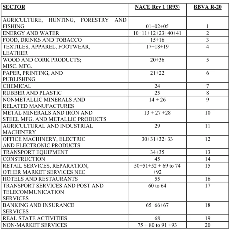
Table A.1. Spanish regions SPAIN ANDALUCIA ARAGON ASTURIAS BALEARIC ISLANDS BASQUE COUNTRY CANARY ISLANDS CANTABRIA * CASTILLE-LEON CASTILLE- LA MANCHA CATALONIA EXTREMADURA GALICIA MADRID MURCIA * NAVARRA (LA) RIOJA * VALENCIAN REGION

Table A.2. Sector categories

SECTOR NACE Rev 1 (R93) BBVA R-20

AGRICULTURE, HUNTING, FORESTRY AND

FISHING 01+02+05 1

ENERGY AND WATER 10+11+12+23+40+41 2

FOOD, DRINKS AND TOBACCO 15+16 3

TEXTILES, APPAREL, FOOTWEAR,

LEATHER 17+18+19 4

WOOD AND CORK PRODUCTS;

MISC. MFG. 20+36 5

PAPER, PRINTING, AND

PUBLISHING 21+22 6

CHEMICAL 24 7

RUBBER AND PLASTIC 25 8

NONMETALLIC MINERALS AND RELATED MANUFACTURES

14 + 26 9

METAL MINERALS AND IRON AND

STEEL MFG. AND METALLIC PRODUCTS 13 + 27 +28 10

AGRICULTURAL AND INDUSTRIAL

MACHINERY 29 11

OFFICE MACHINERY, ELECTRIC

AND ELECTRONIC PRODUCTS 30+31+32+33 12

TRANSPORT EQUIPMENT 34+35 13

CONSTRUCTION 45 14

RETAIL SERVICES, REPARATION,

OTHER MARKET SERVICES NEC 50+51+52 + 69 to 74 +92 15

HOTELS AND RESTAURANTS 55 16

TRANSPORT SERVICES AND POST AND TELECOMMUNICATION

SERVICES

60 to 64 17

BANKING AND INSURANCE SERVICES

65+66+67 18

REAL STATE ACTIVITIES 68 19

TABLES

Table 1. Estimated regional factor productivity differences across regions

π(r) s.e. R2 _{π(r,f) s.e. R}2 _{π(r,f) s.e. R}2 _{π(r,f) s.e. R}2

Andalucia 0.78 0.03 0.93 0.75 0.02 0.93 0.70 0.02 0.78 0.76 0.03 0.89 Aragon 0.80 0.02 0.96 0.77 0.01 0.96 0.63 0.01 0.90 0.81 0.02 0.96 Asturias 0.88 0.04 0.89 0.83 0.02 0.89 0.80 0.03 0.86 0.75 0.03 0.86 Balearic Islands 0.70 0.03 0.92 0.71 0.01 0.71 1.04 0.03 0.85 1.02 0.02 0.61 Canary Islands 1.10 0.03 0.95 1.09 0.03 0.95 1.06 0.04 0.88 1.01 0.03 0.92 Cantabria 0.95 0.03 0.94 0.92 0.02 0.94 1.00 0.02 0.92 0.97 0.03 0.96 Castille-Leon 0.79 0.02 0.96 0.77 0.02 0.96 0.74 0.02 0.91 0.84 0.03 0.96 Castille-La Mancha 0.69 0.03 0.90 0.67 0.01 0.90 0.85 0.02 0.85 0.71 0.02 0.87 Catalonia 1.03 0.01 0.99 1.04 0.01 0.99 1.16 0.03 0.96 1.05 0.02 0.97 Valencian Region 0.85 0.01 0.97 0.85 0.01 0.97 0.91 0.03 0.95 0.85 0.01 0.98 Extremadura 0.60 0.05 0.68 0.57 0.01 0.68 0.68 0.02 0.50 0.58 0.02 0.77 Galicia 0.85 0.03 0.91 0.81 0.02 0.91 0.75 0.02 0.89 0.58 0.02 0.85 Madrid 1.29 0.03 0.96 1.29 0.03 0.96 0.81 0.02 0.96 1.43 0.03 0.88 Murcia 0.88 0.03 0.95 0.85 0.01 0.61 1.11 0.02 0.78 0.81 0.01 0.47 Navarra 0.97 0.02 0.96 0.97 0.03 0.96 0.87 0.02 0.94 0.98 0.04 0.95 Basque Country 1.00 0.03 0.90 1.07 0.03 0.90 1.00 0.03 0.92 1.11 0.05 0.92 Rioja 0.73 0.01 0.98 0.69 0.02 0.98 0.64 0.01 0.58 0.84 0.04 0.91

Hicks-Neutral (HN) estimation Factor Augmenting Industry Neutral (FAIN) estimation

Physical capital (K) High-educ. labour (H) Low-educ. labour (L)

Note: The HN estimated coefficients are from equation (7) in the main text, and the FAIN estimated coefficients are from equation (8) in the main text.

Table 2. Results for tests on the HOV model’s performance

I. Strict model

1.- The HOV Model 2.- The Pairwise HOV Model 3.- The Relative HOV Model

K H L Pooled K H L Pooled K/L K/H L/H Pooled

Sign test 0.35 0.71 0.65 0.57 0.47 0.65 0.54 0.55 0.64 0.60 0.63 0.62

Variance test 0.54 0.81 0.37 0.55 0.59 0.81 0.23 0.55 0.72 0.55 0.71 0.66

Slope test -0.26 0.11 -0.09 0.08 -0.35 0.40 0.02 0.07 0.28 0.17 0.08 0.16

Standard error 0.31 0.39 0.13 0.19 0.04 0.07 0.03 0.02 0.05 0.04 0.05 0.03

R-squared 0.05 0.08 0.03 0.03 0.21 0.11 0.00 0.01 0.11 0.05 0.01 0.04

II. With Factor Productivity Adjustments - Hicks Neutral (HN)

4.- HOV-HN Model 5.- The Pairwise HOV-HN Model 6.- The Relative HOV-HN Model

K H L Pooled K H L Pooled K/L K/H L/H Pooled

Sign test 0.65 0.88 0.71 0.75 0.48 0.65 0.59 0.58 0.64 0.66 0.62 0.64

Variance test 0.87 0.93 0.90 0.90 0.91 0.85 0.79 0.86 0.86 0.67 0.81 0.78

Slope test 0.27 0.43 0.15 0.29 0.11 0.37 0.23 0.27 0.37 0.22 0.17 0.24

Standard error 0.23 0.22 0.24 0.23 0.06 0.05 0.05 0.03 0.05 0.05 0.05 0.03

R-squared 0.08 0.20 0.03 0.09 0.01 0.17 0.07 0.03 0.16 0.05 0.01 0.04

III. With Factor Productivity Adjustments - Factor Augmenting Industry Neutral (FAIN)

7.- HOV-FAIN Model 8.- The Pairwise HOV-FAIN Model 9.- The Relative HOV-FAIN Model

K H L Pooled K H L Pooled K/L K/H L/H Pooled

Sign test 0.65 0.82 0.70 0.71 0.48 0.63 0.57 0.57 0.63 0.63 0.61 0.62

Variance test 0.85 0.88 0.84 0.86 0.88 0.82 0.77 0.83 0.83 0.64 0.78 0.76

Slope test 0.26 0.30 0.13 0.20 0.09 0.32 0.21 0.21 0.33 0.21 0.14 0.22

Standard error 0.22 0.19 0.19 0.19 0.05 0.04 0.04 0.03 0.05 0.04 0.05 0.03

R-squared 0.08 0.14 0.02 0.11 0.01 0.12 0.05 0.00 0.11 0.03 0.00 0.03

Note: The HOV model uses 17 observations per factor and 51 observations in the pooled analysis. The Pairwise HOV model uses 272 (17x16) observations per factor and 816 observations in the pooled analysis. The Relative HOV model uses 272 (17x16) observations per factor pair and 816 observations in the pooled analysis. The sign test, variance test and slope test are explained in the main text. There are three production factors: physical capital (K), high-educated labour (H) and low-educated labour (L).

Table 3. Comparative results of the regional HOV literature

All results for pooled factor data

Davis et al., 1997 Artal et al., 2006 Requena et al., 2008a Spanish regions Strict HOV Model Spanish regions HOV-HNTA Model Japanese regions Spanish regions Spanish regions Sign test 0.57 0.75 0.82 0.75 0.77 Variance test 0.55 0.90 n.r.** 0.67 0.38 Slope test 0.08 0.29 n.r. n.r. 0.11 Standard error 0.19 0.23 n.r. n.r. 0.08 R-squared 0.03 0.09 n.r. n.r. 0.21

Trade vector Total flows Intra-national flows Total flows

This paper*

Intra-national flows

Notes:

(*): Results for the present paper include the preferred HOV specification with the introduction of the Hicks Neutral Technological Assumption (HNTA) in the model.

(**): These authors elaborate on the link between the missing trade puzzle and the universal-FPE assumption, although they do not expressly report a value for the variance test in the Japanese case. n.r.: not reported.

Davis et al., 1997 use three production factors: physical capital (K), high-educated labour (H) and low-educated labour (L). Artal et al., 2006 use four production factors: physical capital (K), high-low-educated labour (H), low-educated labour (L) and land (T). Requena et al., 2008a use six production factors: physical capital (K), high-educated labour (H), low-educated labour (L), R&D capital, arable land and pasture (TA) and woodland (TF).