Contents lists available atScienceDirect
Neural Networks
journal homepage:www.elsevier.com/locate/neunet
2013 Special Issue
Adaptive filters and internal models: Multilevel description of cerebellar
function
John Porrill
a, Paul Dean
a,∗, Sean R. Anderson
baDepartment of Psychology, Sheffield University, Western Bank, Sheffield, S10 2TP, UK
bDepartment of Automatic Control and Systems Engineering, Sheffield University, Sheffield, S1 3JD, UK
a r t i c l e i n f o Keywords: Cerebellum Internal model Adaptive control
a b s t r a c t
Cerebellar function is increasingly discussed in terms of engineering schemes for motor control and signal processing that involve internal models. To address the relation between the cerebellum and internal models, we adopt the chip metaphor that has been used to represent the combination of a homogeneous cerebellar cortical microcircuit with individual microzones having unique external connections. This metaphor indicates that identifying the function of a particular cerebellar chip requires knowledge of both the general microcircuit algorithm and the chip’s individual connections.
Here we use a popular candidate algorithm as embodied in the adaptive filter, which learns to decorrelate its inputs from a reference (‘teaching’, ‘error’) signal. This algorithm is computationally powerful enough to be used in a very wide variety of engineering applications. However, the crucial issue is whether the external connectivity required by such applications can be implemented biologically.
We argue that some applications appear to be in principle biologically implausible: these include the Smith predictor and Kalman filter (for state estimation), and the feedback–error–learning scheme for adaptive inverse control. However, even for plausible schemes, such as forward models for noise cancellation and novelty-detection, and the recurrent architecture for adaptive inverse control, there is unlikely to be a simple mapping between microzone function and internal model structure.
This initial analysis suggests that cerebellar involvement in particular behaviours is therefore unlikely to have a neat classification into categories such as ‘forward model’. It is more likely that cerebellar micro-zones learn a task-specific adaptive-filter operation which combines a number of signal-processing roles.
©2012 The Authors. Published by Elsevier Ltd.
1. Introduction: the chip metaphor
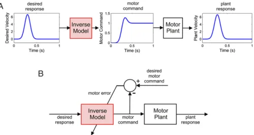
Recent reviews indicate that the possible role of the cerebellum in the formation of internal models is a topic of growing interest (Bastian,2011;Cerminara & Apps, 2011;Ebner, Hewitt, & Popa, 2011;Imamizu,2010;Medina,2011;Shmuelof & Krakauer, 2011). Although the term ‘internal model’ can be used very generally in this context to refer to any neural representation of a dynamic system (Wolpert, Ghahramani, & Jordan, 1995), many of its most important conceptual features can be captured by a simple example (Fig. 1).
Motor commands (as expressed by motoneurons) act on mus-cles which move a part of the body. The mechanical properties of the muscles and body part (for convenience referred to as the mo-tor plant) ensure that the dynamics of the movement differ from
∗Corresponding author.
E-mail address:[email protected](P. Dean).
those of the command (Fig. 1(A)). The circuit shown inFig. 1(B) allows a model of this plant to be learnt, by sending a copy of the motor commands to an adaptive element (highlighted in red throughout). The output of this element is compared with sensory feedback from the actual movement, and the discrepancy between the two used as a signal to ‘train’ the adaptive element (a form of supervised learning). As training proceeds the discrepancy de-creases, meaning that the dynamics of the adaptive element re-semble more closely the dynamics of the motor plant. In this way a model of the motor plant is learnt.
The model shown inFig. 1(usually referred to as a ‘forward’ model, as explained below) has many uses, including the predic-tion of the sensory effects of movement. Such a predicpredic-tion can, for example, help distinguish the sensory signals produced by one’s own movements from those arising from external events—the clas-sical reafference problem (e.g.Cullen, 2004), and further uses are discussed in Section3. Hence proposals that the cerebellum takes part in the formation of internal models seek to provide a crucial link between cerebellar function and proven sensorimotor compe-tences (Blakemore, Frith, & Wolpert, 1999, 2001;Imamizu, Kuroda, Miyauchi, Yoshioka, & Kawato, 2003;Kawato,1995,1996,1999, 2008;Miall, Christensen, Cain, & Stanley, 2007;Miall & Reckess,
0893-6080©2012 The Authors. Published by Elsevier Ltd. doi:10.1016/j.neunet.2012.12.005
Open access under CC BY-NC-ND license.
Fig. 1. Dynamic response and forward model of a simple viscoelastic motor plant. A: The motor command from the motoneurons acts on muscles, which move some part of the body. The mechanics of the muscles plus body part (=‘motor plant’) mean that the temporal trajectory of the movement differs from that of the motor command of the profile of the plant. The example shows the velocity response of a simple viscoelastic plant to a Gaussian motor command. (For convenience, the dynamics of sensory transduction are neglected, so the sensory measurement of the movement introduces no distortions.) B: A circuit for learning a forward model of the motor plant dynamics. The forward model is the adaptive element (highlighted in red; this convention is also applied in later figures). It can be learnt using sensory error (that is, the difference between the predicted and actual sensory consequences of the motor command) as teaching signal. (For interpretation of the references to colour in this figure legend, the reader is referred to the web version of this article.)
2002;Miall, Weir, Wolpert, & Stein, 1993;Miall & Wolpert, 1996; Wolpert,1997;Wolpert & Ghahramani, 2000;Wolpert et al.,1995; Wolpert & Kawato, 1998;Wolpert, Miall, & Kawato, 1998).
To evaluate how far this proposed link is supported by current evidence, the present article first outlines the popular ‘chip’ metaphor for cerebellar organisation, which requires cerebellar functions to be modelled at both microcircuit and external-connectivity levels.
1.1. The ‘chip’ metaphor
The arrangement of neurons and their connections within cerebellar cortex is broadly similar over the entire cortical mantle, whereas each individual region of the cerebellar cortex has a unique pattern of connections with external neural structures. This combination has long been recognised:
‘‘The cerebellar tissues have quite a uniform histological struc-ture. Their role in the actual motor control, however, varies from region to region, depending upon what subcortical structures they are connected with, as pointed out by Herrick (1924)’’ (Ito, 1970, p. 162);
and has given rise to what might be termed the ‘chip’ metaphor of cerebellar organisation
‘‘Cerebellar microcomplexes are connected to various systems of the brain and so play diverse roles in central nervous system functions. This situation would be similar to that of a computer chip which can be used for a great many purposes.’’ (Ito, 1997, p. 475).
This metaphor is illustrated inFig. 2, which shows in schematic form a functional sub-region of cerebellar cortex represented by an identical internal structure and idiosyncratic inputs and outputs. The important implication of the chip metaphor is that the function of any particular cerebellar sub-region depends on
Fig. 2. The cerebellar ‘chip’ metaphor. Each cerebellar microzone has a similar internal organisation, but its own idiosyncratic set of connections, two inputs and one output. The climbing fibre and output connections are unique to a microzone: some of a microzone’s mossy fibre inputs may be shared with other microzones. The climbing fibre teaching signal specifies the learning goals for the chip, hence it is this connectivity which is basic to defining individual microzones. The Purkinje cell output must then be connected to a target region in the deep cerebellar or vestibular nuclei which contributes to achieving this goal, and for which the learning procedure hardwired into the chip is stable and convergent. This provides a strong constraint on the output connectivity. The mossy fibre input connections are the least constrained. They can be regarded as a wide ‘bus’ of possibly relevant sensory and motor signals, from which those signals actually relevant to the task will be chosen by the learning procedure.
boththe signal-processing capacities of the generic chip,andthe particular architecture in which it is embedded.
The relevance of the chip metaphor for evaluating internal-model hypotheses of cerebellar function can be illustrated by the ‘inverse-model’ circuit shown in Fig. 3. The need for an inverse model of the motor plant arises because of the ‘distorting’ effects of plant dynamics on the motor command, as shown inFig. 1(A). Motor commands that specify a desired trajectory for a part of the body must therefore be converted into a form that compensates for the characteristics of the plant. This can be achieved by passing the command, not directly to the plant itself, but indirectly through an inverse model of the plant (Fig. 3(A)). As with the ‘forward’ plant model (terminology emphasising the contrast with the inverse plant model) such a model needs to be learnt, and a possible circuit for achieving this is shown inFig. 3(B). Although, as will be argued later, the circuit shown inFig. 3(B) is too simple to be biologically realistic, it illustrates an important point about the difference between an adaptive element and the circuit of which it is a component. Comparison ofFigs. 1and 3shows how the same adaptive element can learn either a forward model, or an inverse model, depending on the details of the external wiring. This is exactly the point captured by the cerebellar ‘chip’ metaphor ofFig. 2.
Evaluating internal-model hypotheses of cerebellar function therefore entails evaluating both the microcircuit model and the way it is wired into any particular system-level architecture. The particular microcircuit model chosen here is the adaptive filter, and this is briefly described in Section 2, and its general computational suitability for internal model formation explained. Particular internal-model architectures are then assessed in two stages. The first asks how they are biologically plausible—how far the signals they require could be in principle provided biologically (Section3). The second stage considers the problems that arise when the plausible architectures have to be mapped in practice onto complex neural circuits (Section4). The final section addresses the implications of the internal-model hypothesis for the future understanding of cerebellar functions (Section5).
2. Microcircuit level: inside the chip
The repeating nature of the cerebellar microcircuit suggests that there is a generic ‘cerebellar algorithm’, and hypotheses about its computational capability (Albus,1971;Marr,1969) appeared soon after the microcircuit itself was first described (Eccles, Ito, & Szentágothai, 1967). The Marr–Albus framework was further developed by Fujita (1982), who proposed that the cerebellar
Fig. 3. Inverse model control of a simple viscoelastic motor plant. A: A desired plant response, in the form of a Gaussian signal, is transmitted through an inverse model of the viscoelastic motor plant (also used inFig. 1). The inverse model transforms the desired response into the pulse-step motor command that is the exact control input required to reproduce the desired response from the plant. B: A circuit for learning an inverse model of the motor plant dynamics. The inverse model is the adaptive element and can be learnt by using motor error (that is, the difference between actual and desired motor command) as teaching signal as shown in the diagram. Since the desired motor command is not known (or if it was, could be used directly to drive the plant) this inverse model architecture is not biologically plausible as it stands (see text). circuit acts as an adaptive filter in which the mossy fibre inputs to
the cerebellum convey dynamic time-varying signals rather than the static spatial patterns associated with the original Marr–Albus formulations (further details in Section2.4). Since it appears that many of the cerebellar models concerned with behaviour (such as the control of eye or arm movements) resemble the adaptive-filter model (Dean, Porrill, Ekerot, & Jorntell, 2010), this is the microcircuit model considered here. Because the main focus here is on the system-level connectivity, only a brief description is given of the model and its biological plausibility. More detailed analysis is available elsewhere (e.g.Dean & Porrill, 2010, 2011).
2.1. The adaptive filter
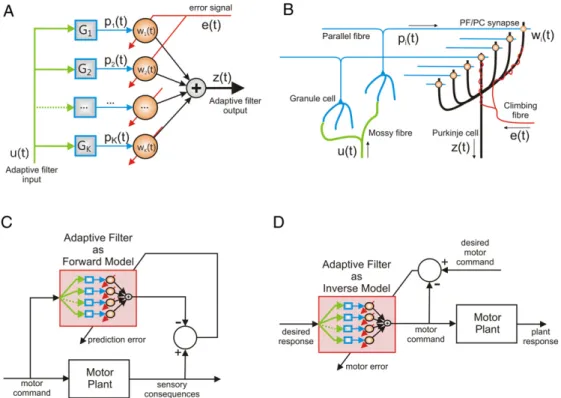
A linear in weights adaptive filter (Fig. 4(A)) takes as input a number of time varying signalsu1
(
t),
u2(
t), . . . ,
uN(
t)
(for clarity only a single input is shown in the figure). These inputs are passed through a basis of fixed filters Gi to produce signalspi=
G[
u1(
t), . . . ,
uN(
t)
]
which are combined with weights(w
1,
w
2, . . . , w
K)
to produce the outputz
(
t)
=
w
ipi(
t).
(1) The term adaptive filter is used because these weights are not pre-calculated, but are changed systematically during the operation of the filter to improve filter performance on a task. The learning rule for filter weights usually takes the formδw
i= −
β
⟨
e(
t)
pi(
t)
⟩
(2)where
β
is a positive learning rate parameter,e(
t)
is called the teaching signal (which is often related to task errors) and the angle brackets denote a time average. This learning rule has been re-discovered in many contexts and given names including the delta rule, the Widrow–Hoff rule (Widrow & Stearns, 1985), the LMS rule, the MIT rule, the covariance rule, etc. We will generally use the term covariance rule (Sejnowski, 1977) since updates to a weightw
iare proportional to the covariance of the signalpi(
t)
controlled by the weight and the teaching signale(
t)
.This learning rule is guaranteed to converge when the teaching signal is the error in filter outputeout
(
t)
=
z(
t)
−
zd(
t)
, but, as we shall see later, this output error signal is not always available to use as a teaching signal. There is some flexibility in the choice of teaching signal however. Suppose we have access to a signale
(
t)
=
H∗
eout(
t)
related to output error by a linear filterH. Thenthe learning rule above will still converge as long as the linear filter His strictly positive real (SPR) (Sastry & Bodson, 1989), that is the phase shift due toH at any frequency must be less than 90° so that the sign of the correlation in the learning rule is not reversed at any frequency. This SPR requirement means, for example, that if learning is required to be stable up to a maximum frequency of 1 Hz then the learning rule can tolerate delays in the teaching signal of up to 250 ms (in general the allowable delay is related to the maximum frequency byT
=
1/
4f; for further discussion see Porrill and Dean(2007a)).The filter shown in Fig. 4(A) is often referred to as an analysis–synthesis filter, with the analysis stage corresponding to the transformation of inputs by the bank of fixed filters, and the synthesis stage corresponding to the subsequent recombination of the suitably weighted transformed inputs.
2.2. Similarity to cerebellar microcircuit
Fig. 4(B) shows the basic cerebellar microcircuit in a form that allows comparison with the adaptive filter shown inFig. 4(A). Mossy fibre inputs carry the signals u1
(
t),
u2(
t), . . . ,
uN(
t)
to the cerebellum; these are analysed by granule cells whose axons bifurcate to form parallel fibres which carry basis signals p1(
t),
p2(
t), . . . ,
pK(
t)
. The parallel fibres synapse on Purkinje cells which perform the linear synthesis to produce the signal z(
t)
carried by the simple spike output. In addition a single climbing fibre winds around the Purkinje cell; spikes on this input cause the PC to fire complex spikes on a 1–1 basis. These complex spikes are interpreted as a trigger for synaptic weight changes with the climbing fibre input acting as a teaching signal. The covariance rule above is broadly consistent with the known behaviour of complex spike dependent LTD and LTP at PF/PC synapse.An important aspect of the resemblance illustrated inFig. 4is that the adaptive filter model offers an explanation of the two dis-tinctive features of the cerebellar microcircuit (e.g.Dean & Porrill, 2011). One is the enormous number of granule cells, estimated at up to 80% of all neurons in the human brain (Herculano-Houzel, 2010), potentially corresponding to the large number of basis func-tions required by an analysis–synthesis filter, particularly if non-linear bases are needed. The second distinctive microcircuit feature is the unusual behaviour of climbing fibres. These produce com-plex spikes in Purkinje cells on average at
∼
1 Hz, apparently too low a frequency to have a significant influence on Purkinje cell out-put (average simple-spike frequency∼
40 Hz). On the other handFig. 4. Adaptive filter model of the cerebellum. A. Systems diagram of the adaptive filter. Input signals (only one is shown for clarity) are analysed by a bank of filters (in engineering applications this could be a bank of delay-lines with a range of delays) to produce a basis of signals; these are recombined with appropriate weights to produce the desired output. The filter weights are adapted over time using the least-mean-squares (LMS) rule. B: Schematic diagram of the cerebellar microcircuit. Mossy fibres transmit the input signal to cerebellar cortex. The granule cell layer transforms the input signal to produce an output transmitted by the parallel fibres. Parallel fibres synapse onto the dendrites of a Purkinje cell. Parallel fibre/Purkinje cell synaptic efficacy is altered by correlational firing of a single climbing fibre and each parallel fibre. C: Forward model approximation of a motor plant using the adaptive filter model of cerebellum. The adaptive filter output is driven by the motor command and the adaptation of filter weights is driven by prediction error. D: Inverse model approximation of a motor plant using the adaptive filter model of cerebellum. The adaptive filter output is driven by the desired response signal and the adaptation of filter weights is driven by the motor error in contrast to (C). This change in connectivity is the only difference between use of the adaptive filter in forward and inverse model roles.
the complex spike produced by a climbing fibre action potential is associated with a large widespread calcium transient through-out the Purkinje-cell dendritic tree, apparently related to plasticity at the estimated 150,000 parallel-fibre synapses on the tree (e.g. Ohtsuki, Piochon, & Hansel, 2009). The peculiar combination of low-frequency firing with very extensive synaptic input that is characteristic of the climbing fibre is exactly what is wanted from a teaching signal which must alter all synaptic weights appropri-ately without contaminating the filter output.
2.3. Biological plausibility of adaptive-filter model
Although the adaptive filter model of the basic cerebellar micro-circuit is popular and appears plausible in certain broad respects, some detailed microcircuit features have been described that ap-pear incompatible with it. For example, some recent studies of granular-layer processing have suggested that mossy fibre signals may be only slightly altered, rather than transformed as required by an adaptive filter. A second example concerns Purkinje cell fir-ing. In certain circumstances Purkinje cells alternate between ‘up’ states with depolarised membrane potential and simple-spike fir-ing, and ‘down’ states with hyperpolarised membrane potential and no simple spikes. In other circumstances, Purkinje cell firing is apparently characterised by complex patterns and pauses, rather than being straightforwardly related to task variables.
Possible explanations for a number of these putative incompati-bilities have been discussed previously (Dean & Porrill, 2010;Dean et al.,2010) with the tentative conclusion that for at least some cerebellar microzones the adaptive filter remains a good candi-date model (Dean, Jörntell, & Porrill, 2013;Dean & Porrill, 2011).
This conclusion appears consistent with a recent review of cere-bellar plasticity (Gao, van Beugen, & De Zeeuw, 2012), which ar-gues that the granular layer increases the diversity of mossy-fibre inputs whereas the Purkinje cell network creates output by select-ing appropriately from this diversity, processes that would seem to correspond well to the analysis and synthesis stages of an adaptive filter. Therefore, since the emphasis here is on circuitry external to the cerebellum, the remainder of the review proceeds on the assumption that this conclusion is correct. The central question considered here concerns the biological plausibility of the adaptive filter as a candidate for the adapting element in forward models as shown inFig. 4(C) and in inverse plant models as inFig. 4(D) (com-pare withFigs. 1(B) and3(B) respectively).
2.4. Computational adequacy of adaptive filter
However, it only makes sense to address questions of biological plausibility if the putative microcircuit algorithm has the required computational power. Can an adaptive filter be used in principle as the learning element in internal model architectures?
A general answer for linear adaptive filters has been provided by Widrow and Stearns (1985), who specifically analysed how they could successfully be used to learn either forward or inverse models, and how such adaptive models could be used for model control, inverse control, interference cancellation, system identification, and signal prediction.
More recent work on the CMAC (Cerebellar Model Articulation Controller) described by Albus (1971) is consistent with this analysis. The CMAC treats the cerebellar microcircuit as a look-up table which stores the desired response to a given set of inputs, and therefore functions as a pattern classifier or feature detector.
However, the learning rule used by the CMAC for adjusting its weights is of the same form as the covariance rule used by adaptive-filter models, so the main difference between the two consists of how inputs are coded. Although Fujita (1982) has claimed that the spatial pattern-classifier used in the CMAC does ‘‘not account satisfactorily for processing of time–analog signals conveyed by frequency-modulated nerve impulses’’ (p. 195), it can be argued that the differences in coding between the CMAC and the adaptive-filter are concerned more with convenience of representation for individual problems rather than a fundamental computational point (Dean et al., 2010).
It turns out that although CMACs are now rarely used for simulating the role of the cerebellum itself (Dean, Mayhew, & Langdon, 1994), they continue to be applied to an extremely wide variety of adaptive control and signal-processing problems (
∼
30 papers per year), including fuzzy control, non-linear control and stock index forecasting (Cheng, 2011; Commuri & Lewis, 1997; Lin, Chen, & Yeung, 2010; Lu & Wu, 2011; Tao & Su, 2011). Of particular relevance here are the CMAC applications to the control of complex robots (Kim & Lewis, 2000;Sabourin, Bruneau, & Buche, 2006). If the above argument concerning CMACs and adaptive filters is accepted, the continuing usefulness of the CMAC in engineering and other contexts can be used as testimony to the computational adequacy of adaptive filters in many control and signal processing architectures, including those required by internal-model hypotheses.3. Chip connectivity: biological plausibility
The second stage of evaluating internal-model hypotheses concerns the system-level connectivity required by an adaptive filter to implement the variety of internal-model architectures that have been proposed for the cerebellum. To make this evaluation process more tractable, we split it here into two stages. First, which specific internal-model architectures arein principlebiologically plausible? Second, do these plausible architecturesin practicemap onto neural circuitry in the ways proposed by the models?
The present section deals with the first of these questions: how far are the proposed circuits biologically plausible, in the sense of requiring input signals that at least in principle could be available in the brain. We consider five specific circuits that have been proposed in the literature. (This section is a much fuller exposition of material covered briefly in Supplementary Material of Dean et al., 2010.)
3.1. Forward models
A forward model of a dynamical system describes the relation-ship between the inputs to the system and its outputs, for example the relationship between the motor commands to a motor plant (e.g. a mechanism consisting of muscles and joints) and the sensory consequences of the movement they produce (Fig. 1). Implement-ing a forward model of a complex motor plant requires a learnImplement-ing element that can accurately simulate complex input–output trans-formations, and in biological systems such models can only be ac-quired by supervised, trial and error, learning. Forward models are thus ideally suited to implementation via an adaptive filter.
A simple architecture in which a forward model can be learned successfully has been shown in Fig. 1. It can be seen that the connectivity requirements are:
1. Mossy fibre input to the forward model consists of an efference copy of the relevant motor commands.
2. The error signal required for learning is error in model output. This signal must be made available on the climbing fibres.
3. In order to calculate the required error signal the model output must target a comparator in which it is subtracted from the actual plant output.
If the teaching signal is output error (i.e. discrepancy between actual and predicted sensory signal) as shown in Fig. 1, then the adaptive filter with covariance learning rule is guaranteed to learn to be an optimal estimate of the plant (in the sense that it minimises the mean square prediction error). Provided sufficient time is available for learning, the accuracy of this estimate is therefore limited only by the completeness of the basis signals generated by the adaptive filter (seeFig. 4(A)).
In engineering systems the architecture shown inFig. 1is very often used, since the forward models learnt can be ‘unplugged’ and used elsewhere. It is difficult to see how this option could be implemented by a biological system. However forward models are often required as components of more complex architectures that can be biologically relevant. It is important to realise that successful learning in these architectures does not follow directly from the simple case described here, and that in each case a separate analysis must be made of the availability of the error signal required for learning, based on the specified connectivity. We will consider three further examples of architectures which include a forward model: noise cancellation in Section 3.1.1, the Smith predictor in Section3.1.2, and the state estimator in Section3.1.3.
3.1.1. Noise cancellation
An important application of forward models in signal process-ing is adaptive noise-cancellation (Widrow & Stearns, 1985). The basic structure of the problem is shown inFig. 5(A). An input signal of interest,s
(
t)
, is corrupted by noisen(
t)
, for example unwanted aircraft noise may leak into a headphone audio signal (Dean et al., 2013). Independent information about the noise source is assumed to be available, in the headphone example from a small micro-phone embedded in the earmicro-phones. This noise-source information, or reference signalr(
t)
, is used as the input to an adaptive filter, whose job it is to provide an estimatenˆ
(
t)
of the actual noise that is present in the signal. Ifr(
t)
andn(
t)
were identical the task would be very straightforward, because the output of the required filter would be identical to its input. However the noise may have been changed before being added to the signal of interest, a process rep-resented in the diagram by the box labelled ‘noise channel’. The task of the adaptive filter is therefore to learn a forward model of the noise channel.Previous analyses would suggest that the required teaching signal is filter output errore
(
t)
= ˆ
n(
t)
−
n(
t)
, but this is clearly unavailable since we have no access to the ‘true’ noise signaln(
t)
. An alternative teaching signal can be derived by considering a slightly unusual performance measure, the power of the predicted signalsˆ
(
t)
, given by E=
1 2
ˆ
s2
.
(3)Expanding
ˆ
s(
t)
and assuming statistical independence between both noise and reference noise and the signals(
t)
givesE
=
1 2
ˆ
s2
=
1 2
(
s+
(
nˆ
−
n))
2
=
1 2
s2
+
1 2
(
nˆ
−
n)
2
(4) (since other cross-correlation terms vanish). Hence this cost function is equal to mean square output error plus a constant, so minimising it minimises output error. Its gradient is∂
E∂w
i=
ˆ
s∂
ˆ
s∂w
i
=
ˆ
spi
(5)Fig. 5. Adaptive cancellation of reafferent signals. A: Adaptive noise cancellation architecture. The problem addressed in noise cancellation is to suppress noisen(t)that additively corrupts a signal of interests(t). Aknownreference noiser(t), which is correlated with theunknowndisturbance noise, is used to drive a forward model of the noise channel. The predicted noise signalnˆ(t)produced by the forward model is used to cancel the noise from the observed signal, resulting in a predictionˆs(t)of the signal of interest, this signal also acts as teaching signal. The architecture is adaptive, so that the forward model can track changing dynamics of the noise channel. B: Reafferent signal cancellation. During active sensing reafferent signals are often generated that can interfere with the detection and analysis of exafferent signals. The adaptive noise cancellation architecture in (A) can be used directly to overcome the reafference problem by substituting motor commands for reference noise. Hence, in a biological scenario the animal or human can learn to predict the sensory consequences of their own movements and cancel these reafferent components from observed sensory signals. so the gradient descent learning rule is a covariance learning rule
δw
i= −
β
ˆ
s(
t)
pi(
t)
(6) where the teaching signal ise(
t)
= ˆ
s(
t)
. This learning rule adjusts the weights until the estimated signal is uncorrelated with all the componentspi(
t)
of the reference noiser(
t)
. This is an informative example, because the teaching signal we have derived is clearly not a performance error, in fact it is the signal of interest. This means that it also provides an example where successful learning does not reduce the signal carried on the climbing fibre to zero, as would be expected for an error signal.This architecture shown can be applied directly to the problem of predicting the sensory effects of movement in biological systems (Fig. 5(B)). The signal of interest is now the output of a biological sensor. The task is to separate sensory signals that are produced by events in the outside world (exafference) from the ‘noise’ generated in the sensor by the animal’s own movements (reafference). The nature of this contamination cannot be known directly, but there is information about the movements themselves, provided by the motor commands sent to the relevant muscles. This ‘efference copy’ information is in effect reference information about the noise source, and so could be used as input to an adaptive filter (possibly located in the cerebellum, see below) that learns to mimic the transformation of motor commands into sensory signals. Thus the cerebellum would learn a forward model of ‘Plant
+
Sensor Dynamics’, including its basic properties of elasticity, viscosity and inertia, together with any post-processing in the sensory apparatus.Once learning has been achieved, the adaptive filter output is an explicit prediction of the effects of the animal’s own movements on the sensory signal. This prediction is subtracted from the raw sensory input to provide an estimate of the sensory signal generated by objects in the external world. Learning to predict the sensory effects of movement has been suggested as a central cerebellar function (e.g.Miall & Wolpert, 1996). A homely example concerns the difficulty of tickling oneself: the argument is that this difficulty is caused by a prediction of the sensory effects of one’s own movement that is used to diminish the actual sensory effects (Blakemore, Wolpert, & Frith, 1998).
The connectivity requirements for a hypothetical noise cancel-lation module are thus:
1. Mossy fibre input to the cerebellum is an efferent copy of the motor commands.
2. The error signal required for learning is the noise-cancelled signal.
3. Cerebellar output is an estimate of the self-produced sensations caused by the animal’s own movement, and must target a comparator to produce the noise-cancelled signal. Efferent copy of this signal must be available on the climbing fibre to provide the teaching signal inFig. 5.
The signals required by the adaptive element in this architec-ture appear to be available biologically, and its computational ef-fectiveness has been tested in the context of a rat-like whisking robot, using only observed whisker signals and a copy of motor commands as inputs (Anderson et al., 2010). The next question therefore concerns whether the circuit is in fact implemented bi-ologically. This question is addressed in Section4, for a particu-lar form of noise cancellation that can be used for the detection of novel stimuli.
3.1.2. Smith predictor
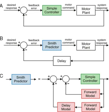
In engineering systems the preferred control option for track-ing a desired response in a motor system is usually a feedback con-troller as shown inFig. 6(A). The motor plant output is compared with the desired response and the error is fed into a high-gain con-troller (labelled ‘simple concon-troller’ inFig. 6(A)) to produce the re-quired motor command. To achieve stable and accurate tracking of time varying signals requires careful choice of controller, and there are powerful standard techniques for designing such controllers when a plant model is known.
However if the plant output is subject to delay the use of high-gain controllers can lead to instability and these standard control design techniques break down. In the control engineering literature a scheme known as the Smith predictor (Fig. 6(B)) is often used to overcome the problems associated with designing feedback controllers for systems with delay. The key benefit to the designer is that it allows a simple controller to be designed for the delay-free plant using standard methods. This controller is then used as a component in the Smith predictor (Fig. 6(C)) which also requires a forward model of the plant and a model of the delay. This architecture is guaranteed to give stable control of the delayed plant when the plant and delay models are accurate.
It has been suggested (Miall et al., 1993) that the cerebellum could act as a Smith predictor, compensating for the unavoidable time-delays arising from sensorimotor transmission and central processing of neural signals in biological systems. It is important in assessing this suggestion to make Marr’s distinction between the computational and the algorithmic levels of description. Computationally the Smith predictor implements a control scheme in which the desired response is reproduced with a fixed temporal delay. It is plausible that such a controller could be learned directly by the cerebellar microcircuit in a suitable architecture and
Fig. 6. The Smith predictor. A: Feedback control loop. A controller driven by feedback error causes a motor plant to track a desired response. This control architecture is widely used in engineered systems, and there are standard procedures for designing suitable controllers when the plant is not subject to delay. B: The Smith-predictor control loop. The control loop is now complicated by the presence of a delay, here shown in the sensory feedback pathway. The presence of a delay complicates control but a Smith predictor can be used to simplify the design process, which in effect allows the engineer to use a simple controller designed for a plant without delay. Note that for linear systems, the sum total of delays through a control loop (motor, sensory and plant) can be lumped into a single delay component, which has an equivalent effect on control performance when placed at any location in the loop. C: Smith-predictor controller architecture. The Smith predictor comprises two forward models of the plant, one with delay and one without. Motor commands are primarily generated through control of the undelayed forward model (the inner loop), thereby avoiding control problems associated with delay. However, the sensory feedback loop shown in (B), is required for the compensation of disturbances. Therefore, the outer loop of the Smith predictor (through the delayed forward model) is used to cancel the feedback error for zero disturbances, which permits the transmission of unpredictable disturbances only to the inner control loop (assuming an exact forward model of the plant).
this possibility should be investigated. However the term Smith predictor implies a particular algorithm based on the architecture shown inFig. 6(C) (or one of its variants) with specific modules implementing the forward plant and delay models found in that diagram. We are not aware that any biologically plausible scheme has been proposed that would allow these individual modules to be learned stably. For example, the teaching signal necessary for learning the plant forward model in Fig. 6(C) is the difference between the model input and the undelayed plant output, and the teaching signal necessary for learning the delay model is the difference between the (true) delayed and undelayed plant outputs. Neither signal appears in any natural way in the Smith predictor architecture, and substitution of similar signals containing the delayed components will necessarily lead to learning instability. Some of the stability problems in learning with delayed signals might be countered by a synaptic eligibility trace whose delay matched the plant delay accurately (Porrill & Dean, 2007a) but since this delay is an intrinsic property of the parallel fibre/Purkinje synapse, it could only cope with a limited range of delays (e.g. up to 200 msWang, Denk, & Häusser, 2000).
In the light of this analysis we highlight a number of challenges facing the Smith predictor hypothesis for which computational models have yet to be proposed: (i) How is anundelayedforward model learnt from signals that are necessarily delayed by
efferent/afferent processing? (ii) How is the Smith predictor architecture specifically subdivided in terms of forward model components and delays? (iii) In this architecture, what is the role and connectivity of the cerebellum? (iv) How are sensory error signals distributed in order to drive learning in separate Smith predictor components (forward model and delay model)? Answering these questions could well provide key insights into the handling of efferent/afferent delays in motor control.
In addition the configuration shown inFig. 6(C) requires sepa-rate models of the controlled plant and of the delay (Miall et al., 1993) suggested a slightly more plausible organisation but one in which the plant and delay are still represented separately). This modular configuration is an unlikely outcome of learning with plausible teaching signals, since it requires a division of the sensory error into individual components due to errors in plant and de-lay models. Although it seems unlikely that regions of the cere-bellum correspond in any direct way to the modular components implied by the Smith predictor architecture, it would be interesting to investigate whether individual components of this architecture – for example the loop via a forward model, which is very similar to the internal feedback loop proposed by Robinson (e.g. Robin-son, 1981) for the control of saccades – have plausible cerebellar implementations.
3.1.3. State estimator
The input–output characteristics of a system such as a motor plant often depend on the past history of the control inputs as well as their current values. The state vector of such a system is defined to be a set of variables which completely describes the system, including these ‘historical influences’, such that the control inputs, together with the initial state, completely determine the future behaviour of the system. Physical output from the model can be regarded as a measurement of some combination of these internal state variables. Having access to the internal state of a system is very useful when designing controllers and has important theoretical consequences. For example it can be shown that the optimal controller for many stochastic systems can be implemented as a feedback controller with access to the internal state (Todorov, 2005).
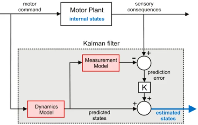
If an accurate theoretical model of the system is unavailable the only way to determine its internal state is by inference from measurements on the system. When the system is linear an optimal (in the sense of least squares) algorithm for state estimation is known, which can be implemented using a Kalman filter in the architecture shown inFig. 7.
Implementation of this state-estimator requires a great deal of knowledge about the observed system. Firstly we need to know the state update model, which describes how the internal state of the plant changes over time both autonomously, and under the influence of control inputs and system noise. We also need the measurement model, which describes how measurable quantities are related to the system’s internal state, and also includes a model of measurement noise. The state estimator uses these two models to estimate the system’s current state; updating the current estimate of the state vector over time using the state update model and improving this estimate when new measurements arrive. This process uses a Kalman filter algorithm, which determines the optimal values for the gain matrix which determines the influence of the current measurements on the state-estimate. Clearly this influence should be small when the measurements are inaccurate relative to the expected error in the internally predicted state, but large in the opposite case. In essence the Kalman gains determine the relative weighting to be given to the estimates from internal models compared to external measurements.
Kording, Tenenbaum, and Shadmehr(2007) have investigated the use of state estimation in biological motor control systems
Fig. 7. The Kalman filter. Architecture of a Kalman filter state-estimator. The Kalman filter combines predictive information with sensory observations to produce an optimal estimate of the plant’s internal state. The predictive element of the Kalman filter is similar to a typical forward model but the forward model is split into two components: (i) a dynamic state model that predicts future states from current values – the dynamics model, and (ii) a static model that maps states to sensory signals – the measurement model (each highlighted in red, since they could be learned adaptively). The motor commands that drive the plant are also provided as input to the dynamics model to predict the next state. When measurements become available the predicted state is additively combined with the sensory prediction error weighted by the Kalman gain matrix (K), to produce an improved state estimate. (For interpretation of the references to colour in this figure legend, the reader is referred to the web version of this article.)
in the context of saccadic gain adaptation. Saccades become inaccurate if the gain of the saccadic plant varies over time. Such gain changes can arise from a variety of internal causes such as muscle fatigue, or developmental changes in muscle strength. These individual components of the muscle state can have different characteristic time constants and sizes. For example fatigue may cause large, relatively rapid variations while developmental changes cause slower, smaller variations. Although observing saccadic performance only gives information about the combined effect of these components the Kalman filter architecture outlined inFig. 7is capable of estimating the contributions of the individual components and making an optimal gain estimate. Comparing the behaviour of this ‘ideal observer’ with actual performance has shown that in many cases the gains used by real observers are the optimal gains characteristic of state estimation methods.
Studies of this kind can indicate that the system as a whole can approximate state-estimation, but do not indicate whether the site of state-estimation is, as has been proposed, the cerebellum (Miall et al., 2007; Miall & Wolpert, 1996). As far as we are aware no detailed mechanisms or architectures for the biological implementation of state estimation methods have been proposed, so we are unable to give a detailed analysis of the required connectivity or learning characteristics. In particular, no scheme has been suggested that could implement the detailed matrix equations required to estimate the optimal Kalman gain matrices required in the general case.
The argument so far has focused on state-estimation in the context of hidden or unobservable states of a motor plant, states which may in engineering applications have no physical em-bodiment whatsoever but which have direct relevance to motor control. However, state-estimation as a generic process for com-bining measurements and model-based predictions can be applied to a very wide range of tasks, including prey localisation (by pre-cerebellar structures in electric fishPaulin, 2005) or estimating the position and velocity of an arm (Miall & Wolpert, 1996). Since the state update model in Fig. 7is essentially a forward plant model which has to be adaptive to track the true plant, it could in principle be implemented as a (cerebellar) adaptive filter. Per-haps an approximation to the required Kalman gains could also be implemented with an adaptive filter (thoughPaulin, 2005used
3.2. Inverse models
We have seen that a feedforward controller can be imple-mented using the architecture shown inFig. 3(A). As implemented in its simplest form inFig. 3(B) this requires the cerebellar adaptive filterCto learn the inverseC
=
P−1of the motor plantP, hencethe name adaptive inverse control.
In the architecture shown in Fig. 3(B) the teaching signal required for supervised learning is the error in adaptive filter output, sometimes called proximal error. Although this error in filter output causes the errors in system output (distal or sensory error) that will be measured by sensors, the two are not usually related in a simple way. The fact that it is only sensory (distal) error that is directly available to a learning system rather than learning element output (proximal) error is called the distal error problem: it is a generic problem in neural net learning systems (Jordan,1996; Jordan & Wolpert, 2000).
In motor systems, if an adaptive-filter output contributes to a motor command, its output error is called motor error. In this case the distal error problem is also called the motor error problem, and is directly relevant to the issue of biological plausibility of cerebellar internal models. InFig. 3(B) the teaching signal required is motor error—the difference between actual and desired motor commands to the motor plant. As we have noted this error signal is not directly observable since it passes through the motor plant before producing observable sensory consequences. Nor can the desired motor commands be known in advance in biological systems—hence the circuit shown inFig. 3(B) as it stands is not biologically plausible.
Two basic solutions to the motor error problem for cerebellar learning have been proposed, motor error learning (Section3.2.1) and recurrent architecture (Section3.2.2). In both cases we must take account of the cerebellum acting in conjunction with other control pathways since cerebellar lesions do not completely abolish function. This arrangement appears to be a general feature of cerebellar control, as seen for example in the vestibulo-ocular reflex (Section4.2.2) where the supplementary controller can be localised in the brainstem (for this reason we will term this non-cerebellar componentB).
3.2.1. Motor error learning
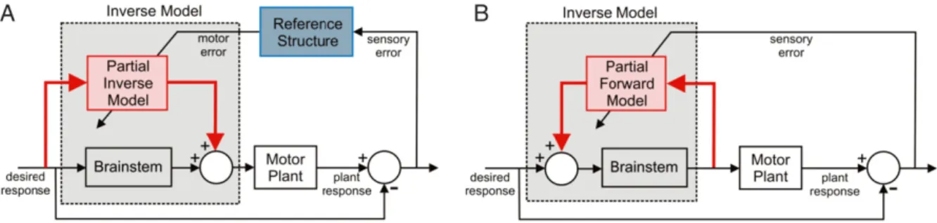
The first solution tackles the motor-error problem head on: the required motor error is calculated from sensory errors by hypo-thetical neural structures called reference structures (Fig. 8(A)). This approach has been most strongly advocated by Kawato and co-workers and implemented in the feedback–error–learning al-gorithm (Gomi & Kawato, 1992, 1993;Kawato & Gomi, 1992, 1993), where the estimated motor error can also be used in online feed-back mode to improve movement accuracy (not shown in figure). In this architecture, taking into account the contribution fromB, the cerebellum learns a partial inverse model,C
=
P−1−
B.Because motor error is related to sensory error by the plant transfer function P, sensory error is not a satisfactory training signal unless the plant itself satisfies the Strictly Positive Real con-dition (Section3.1). This constraint severely limits the applicabil-ity of the circuit shown in Fig. 8(A) if sensory error were used directly as a teaching signal, especially in multi-joint configura-tions. Feedback–error–learning attempts to solve this problem by
Fig. 8. Alternative architectures for adaptive inverse plant compensation. A: Motor-error architecture. The motor command is produced by a combination of a fixed element (calledBin the text and representing e.g. the brainstem in the case of the VOR) and an adaptive elementCrepresenting the cerebellum. Together the fixed and adaptive components combine to form an inverse modelP−1=B+Cof the plant. In order to learn the partial inverse modelC=P−1−B, the required teaching signal is motor
error. However, the motor error is unavailable, and therefore must be estimated from the sensory error by filtering the sensory error through a reference structure that approximates an inverse model of the plant. Since an (approximate) inverse model of the plant must be known in order to learn an inverse model of the plant this reasoning is circular for all but very simple plants. B: Recurrent architecture. This differs from (A) in the direction of the cerebellar arcs (highlighted in red). The cerebellum receives copies of motor command as input and its output is added to the desired response signal. Unlike the forward architecture in (A), the sensory error is used directly, thus avoiding the circularity mentioned above. Although the brainstem and cerebellum combined constitute an inverse model, the cerebellum itself learns a partial forward modelC=B−1−P. (For interpretation of the references to colour in this figure legend, the reader is referred to the web version of this article.)
‘back-propagating’ sensory error through an approximate inverse of the motor plant (as shown by the blue box labelled ‘Reference Structure’ inFig. 8(A)) to obtain an estimate of motor error. Hence the connectivity requirements for this architecture are:
1. Mossy fibre input to the cerebellum consists of a copy of the desired motion.
2. The error signal required for learning is motor error. This signal must be made available on the climbing fibre by passing the sensory error through a suitable reference structure.
3. Cerebellar output must target a brain region involved in transmitting the motor command, and makes an open-loop contribution to this command.
Fig. 8(A) illustrates the central problem with this scheme, which is the requirement for an inverse model (in the Reference Structure) to learn an inverse model. Feedback–error–learning seeks to escape this apparent circularity by using a relatively simple approximation to the true inverse model, such as a single gain term to transform sensory into motor error.
However, although such approximations have been shown to work well in particular theoretical and robotics contexts (e.g.Dean, Mayhew, Thacker, & Langdon, 1991;Kawato, Furukawa, & Suzuki, 1987;Kawato & Gomi, 1993;Miyamura & Kimura, 2002;Nakanishi & Schaal, 2004) they run into problems for more complex plants. Thus, a feedback–error–learning model of the cerebellar control of reaching movements requires that inferior olivary cells ‘‘detect ‘torque-like’ errors in performance’’ (Schweighofer, Spoelstra, Arbib, & Kawato, 1998, p. 99), and a recent application of feedback–error–learning to control of 7-dof robot arm (Tolu, Vanegas, Luque, Garrido, & Ros, 2012) uses a teaching signal explicitly related to individual errors in joint angle. The inescapable difficulty is the general constraint that the reference structure required for stable learning (i.e. an implicit inverse Jacobian) be of similar complexity to the inverse model. This point has been made in the context of robotics (e.g.Porrill & Dean, 2007b), with the claim that feedback–error–learning ‘‘is rarely used in the literature’’ (Schenck, 2011, p. 8). For biological plants it has been argued that with multiple-input multiple-output redundant systems such as the vestibulo-ocular reflex in three dimensions, the connectivity needed by the reference structure becomes infeasibly complex— how exactly should a vertical retinal-slip signal be channelled to the six oculorotatory muscles (e.g. Fig. 3 ofPorrill, Dean, & Stone, 2004)? AsGomi and Kawato(1992,p. 112) point out: ‘‘The most interesting and challenging theoretical problem (raised by FEL) is setting an appropriate inverse reference model in the feedback controller at the spinal and brainstem levels’’.
A second drawback of the architecture shown in Fig. 8(A) is that it requires the climbing-fibre signal to cerebellar cortex to be an estimate ofmotor error. ‘‘Our view that the climbing fibers carry control error information, the difference between the instructions and the motor act, is common to most cerebellar motor-learning models; however ours is unique in that this er-ror information is represented in motor-command coordinates’’ (Gomi & Kawato, 1992, p. 112). However, experimental investiga-tions of climbing-fibre signals have emphasised their sensory na-ture (see e.g.Miall & Wolpert, 1996), related to touch, pain, mus-cle sense, or in the case of the vestibulo-ocular reflex retinal slip (references inPorrill & Dean, 2007b). The fundamental importance of this sensory signalling is reflected in the zonation scheme for cerebellar cortex, which derives from the organisation of inputs to cortex from the inferior olive that are segregated according to the sensory signals they convey (e.g.Voogd, 2011).
3.2.2. Recurrent architecture
The second proposal for a biologically realistic version of Fig. 3(B) uses a recurrent architecture (Fig. 8(B)) in which the input to the adaptive filter is a copy of the motor commands sent to the plant (Dean, Porrill, & Stone, 2002; Jordan,1996; Porrill et al., 2004). This circuit is based on the actual connectivity of particular cerebellar microzones such as the flocculus. It can be shown that with this connectivity learning using sensory error is stable without the need for reference structures, for example by Lyapunov analysis (Porrill & Dean, 2007b). Note that in this configuration the cerebellum converges toC
=
B−1−
P, so that,despite the fact that theoverallarchitecture embodies an adaptive inverse controller (Fig. 8(B)), the cerebellum itself implements an incremental forward model of the plant. This complexity emphasises that the precise nature of the model learnt by the cerebellar chip cannot be predicted without close analysis of the system connectivity.
The connectivity requirements for the recurrent configuration are:
1. Mossy fibre input to the cerebellum is an efferent copy of the motor commands.
2. The error signal required for learning is sensory error in model output (so no reference structure is required).
3. Cerebellar output must target the brain region producing the desired motion command, forming a closed-loop or recurrent architecture.
This architecture, which is consistent with a range of anatomi-cal and neurophysiologianatomi-cal evidence, has previously been shown
(Middleton & Strick, 2000) of unknown function (Ramnani & Miall, 2001). The computational analysis presented here provides a pos-sible answer. Cerebellar loops allow stable adaptive learning using only observable sensory errors. This allows the cerebellar microcir-cuit to be treated as a ‘cerebellar chip’ which can be plugged into a motor system to improve performance, without the need for com-plex, hard-wired reference structures.
3.3. Conclusions
This section has considered five architectures, three relating to forward models and two to inverse models. We argue that three of these architectures – at least in their present forms – appear to require signals that are not available biologically. The two architectures that do seem to be biologically plausible in principle, namely noise cancellation (forward model) and the recurrent architecture (inverse model) are considered further in the next section, which asks whether they are in fact implemented in neural circuitry. Here we address the distinction between the adaptive filter architectures suitable in engineering applications and those suitable for biological systems. The following appear to be important differences between biology and engineering.
1. The learning rule in biological systems is fixed by the charac-teristics of synaptic plasticity in the microcircuit. It cannot be adaptedad hocto suit particular tasks, in the way engineers might choose specific methods from an extensive toolkit, for ex-ample supplementing an adaptive back-stepping design with a particular anti-windup scheme, to meet the needs of a specific task.
2. The cerebellar chip metaphor should not be over-extended. In engineering applications it is possible to learn a particular com-ponent, such as an inverse model (this learning will often be off-line) and then plug the learned component into another slot in a control architecture. In contrast current evidence suggests that the cerebellar chip must learnin situ, and must continue to function during the learning process. If correct this simple ob-servation rules out many commonly used engineering solutions to control problems.
3. The teaching signals required for adaptive control and signal processing must be biologically plausible. In many cases these signals will indicate performance errors (but not always, cf. noise cancellation) since these indicate the need to change sys-tem parameters. These errors will be provided originally by bio-logical sensors, such as vision or touch, and they should as far as possible be used as teaching signals without requiring extensive processing based on task characteristics (in the way that engi-neers can choose between output error, equation error, filtered error, etc.). Although this criterion precludes the use of the com-plex reference structures required to recover motor error it does not exclude the possibility that extensive pre-filtering, together with other operations such as signal gating is implemented in pre-olivary structures.
4. Chip connectivity: biological implementation
In this section we investigate to what extent the two architectures that seem biologically plausible in principle, namely noise cancellation (forward model) and the recurrent architecture (inverse model), are implemented by neural circuitry in practice.
accompanied by descriptions of the detailed neural circuitry that would be required for such a role. Assessing how far noise-cancellation is in fact carried out by a cerebellar model is therefore a difficult task. Here we consider two possible examples. The first is a hypothesis concerning the circuitry underlying a particular variant of noise-cancellation involving the cerebellum, namely detection of novel vibrissal inputs by the whisking rat. The second concerns experimental evidence directly implicating cerebellar-like structures in noise cancellation in electric fish.
4.1.1. Noise cancellation and novelty detection
The architecture for novelty detection shown in Fig. 9(A) is similar to that of Fig. 5(B), but with the addition of a copy of the sensory signal being sent to the adaptive element. The specific application considered here is the detection of unexpected whisker contacts by rats, so the components of Fig. 5(B) have been re-labelled appropriately. Since the adaptive filter now has information about previous sensory inputs, it is able to cancel any component of the signal predictable from its past history. That is, it becomes a novelty detector, responsive in the whisking application only to new contacts, or sharp changes in the characteristics of a contact.
The connectivity requirements for a novelty-detection module are therefore:
1. Input to the adaptive filter is an efferent copy of the relevant motor commands, together with the original sensory signal. 2. Filter output is an estimate of self-noise, and must target a
comparator to produce the noise-cancelled signal.
3. The efferent copy of this signal provides the teaching signal for the filter.
The signal from the whiskers is contaminated by ‘self-noise’ signals that are generated by the animal’s own exploratory movements of the whiskers (‘whisking’). The nature of this contamination cannot be known directly, but there is information about the whisking movements themselves, provided by the motor commands sent to the muscles that move the whiskers. This ‘efference copy’ information in effect is the reference information about the noise source, and so can be used as input to an adaptive filter (with proposed location in zone A2 of the cerebellum) that learns to mimic the transformation of motor commands into sensory signals from the whiskers. Thus, the cerebellum learns a forward model of ‘Plant
+
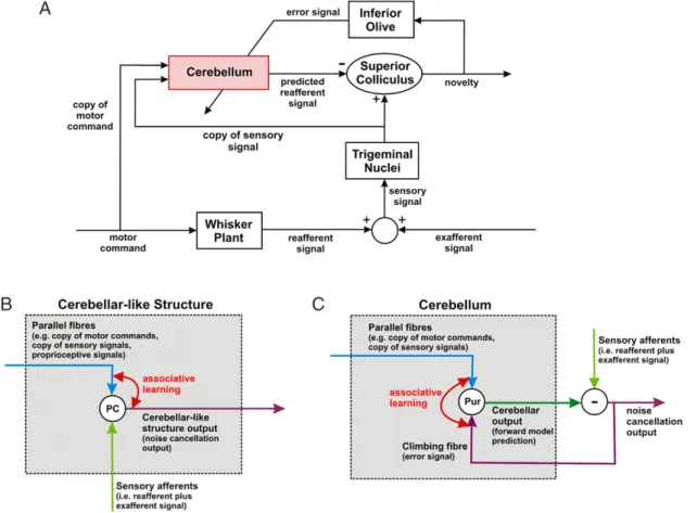
Sensor Dynamics’, including its basic properties of elasticity, viscosity and inertia, together with any post-processing in the sensory apparatus (Anderson et al., 2012).Once learning has been achieved, cerebellar output would be an explicit prediction of the sensory signal including the effects of the animal’s own movements on the sensory signal provided by the whiskers. Evidence suggests that this prediction could be subtracted in the superior colliculus from the raw sensory input to provide an estimate of unexpected whisker signal generated by objects in the outside world. The circuit shown inFig. 9(A) is consistent with the known connectivity of the superior colliculus, inferior olive and cerebellum in rat, and with the established role of the superior colliculus in detecting (and orienting to) novel vibrissal stimuli. Further experiments are needed to establish whether it corresponds to the firing patterns of the relevant neurons in those structures (Anderson et al., 2012).
The novelty detection architecture illustrates an important theoretical point. To a large extent the function of a cerebellar chip is fixed by its climbing fibre input and its output target. In
Fig. 9. Possible neural implementations of forward model architectures. A: Novelty detection in rat whisker system. The basic circuit is that shown inFig. 5(B), with the addition of a sensory input to the adaptive filter, re-labelled with proposed neural equivalents. Exploratory movements of a rat’s whiskers (‘whisking’) produce reafferent whisker signals that combine with signals from the external world. A copy of the whisking commands, together with a copy of the contaminated whisker signal, is sent to the cerebellum (zone A2). Climbing fibre input to that zone comes from the superior colliculus via the caudal medial accessory olive. The superior colliculus compares actual and predicted whisker input (the latter from the dorsolateral protuberance of the deep cerebellar nuclei). Discrepancies signal novel whisker contacts, and can be used to initiate movements such as orienting turns of the head (further details inAnderson et al., 2012). B: Forward model for noise-cancellation implemented by cerebellar-like structure in electric fish. Apical dendrites of output cells receive input from parallel fibres carrying signals such as corollary discharge of the electric organ and proprioceptive signals reporting body movement. Basilar dendrites receive input from the periphery—sensory afferents that carry e.g. electroreceptive information contaminated by reafferent signals. The parallel-fibre synapses are plastic, with associative learning being driven by the correlation between output cell firing and the parallel fibre inputs to form a forward model. The forward model prediction is then subtracted from the contaminated sensory signals that arrive via the basilar dendrites, to provide a prediction of the exafferent signal. C: Simplified diagram of the architecture in panel A to emphasise similarities with panel B. In contrast to the cerebellar-like structure, the cerebellar output is the forward model prediction of the reafferent signal. An additional structure is therefore required to act as comparator to predict the exafferent signal, and an additional pathway is required to feed the error signal back to the Purkinje cell to drive associative learning—the climbing fibre.
most applications changes to the mossy fibre filter only affect the completeness of the basis inputs available to the filter and so affect the accuracy of the learned filter output but leave its qualitative character unchanged. However in this example supplying further sensory information on the mossy fibres changes the qualitative behaviour of the learned system: from noise cancellation to novelty detection. The learned internal model is no longer simply a forward model of the whisker dynamics and sensors, but also includes prediction of future sensory inputs from current sensory state and relevant motor information. This kind of hybrid internal model, which reflects properties of both the organism and its environment may be important, since the problem of combining noisy and delayed sensory information with knowledge of self-generated body motion is fundamental, as emphasised by Munuera, Morel, Duhamel, and Deneve(2009).
4.1.2. Cerebellar like structures
Noise-cancellation has been proposed as a function for some ‘‘cerebellar-like’’ structures, such as the electrosensory lateral line lobe (ELL) of mormyrid electric fish. In particular, it has been argued that these structures adaptively remove self-generated interference from the electroreceptor signal (Bell, Bodznick, Montgomery, & Bastian, 1997; Bell, Han, & Sawtell, 2008;
Montgomery, Bodznick, & Yopak, 2012; Requarth & Sawtell, 2011). Output cells (Fig. 9(B)) receive (i) corollary-discharge and proprioceptive information from neurons in the granular layer that form synapses with their apical dendrites and (ii) direct sensory information from their basal dendrites. The synapses on the apical dendrites are plastic, and their weights are adjusted according to the correlation between the firing of their parent parallel fibre and the firing of the principal cell. The Anti-Hebbian rule for adjusting the weights is similar in form to that used here (Roberts, 1999), with the result that the sum of the weighted granule layer inputs comes to form a negative image of the self-generated interference. This is combined with the actual sensory input arriving at the basal dendrites, so that the output of the principal cell forms an estimate of the uncontaminated sensory signal (Roberts & Bell, 2000;Sawtell & Williams, 2008).
One important difference between the cerebellar (Fig. 9(B)) and cerebellar-like architectures (Fig. 9(C)) is that the output layer cells in cerebellar-like structures embodyboththe adaptive filter and the comparator of predicted and observed sensory signal. This arrangement has the advantage that the firing rates of these cells can be used directly as a teaching signal, whereas the more complex arrangement ofFig. 9(A) requires an indirect teaching signal to be conveyed to the cerebellar Purkinje cell by the climbing