A Primal-Dual Algorithmic Framework for Constrained Convex Minimization

A Primal-Dual Algorithmic Framework for Constrained

Convex Minimization

Quoc Tran-Dinh

•

Volkan Cevher

Laboratory for Information and Inference Systems (LIONS),

´

Ecole Polytechnique F´ed´erale de Lausanne (EPFL), CH1015 - Lausanne, Switzerland.

{quoc.trandinh, volkan.cevher}@epfl.ch.

March 3, 2015

Abstract

We present a primal-dual algorithmic framework to obtain approximate solutions to a prototypical con-strained convex optimization problem, and rigorously characterize how common structural assumptions affect the numerical efficiency. Our main analysis technique provides a fresh perspective on Nesterov’s excessive gap technique in a structured fashion and unifies it with smoothing and primal-dual methods. For instance, through the choices of a dual smoothing strategy and a center point, our framework subsumes decomposition algorithms, augmented Lagrangian as well as the alternating direction method-of-multipliers methods as its special cases, and provides optimal convergence rates on the primal objective residual as well as the primal feasibility gap of the iterates for all.

Keywords: Primal-dual method; optimal first-order method; augmented Lagrangian; alternating direction method of multipliers; separable convex minimization; monotropic programming; parallel and distributed algorithm.

1

Introduction

This article is concerned about the following constrained convex minimization problem, which captures a surprisingly broad set of problems in various disciplines [11, 18, 43, 70]:

f?:=min

x {f(x):Ax=b,x∈X}, (1)

where f :Rn→R∪ {+∞} is a proper, closed and convex function; X ⊆Rn is a nonempty, closed and

convex set; andA∈Rm×nandb∈Rmare known. In the sequel, we develop efficient numerical methods to

approximate an optimal solutionx?_{to (1) and rigorously characterize how common structural assumptions on}

(1) affect the efficiency of the methods.

1.1

Scalable numerical methods for

(1)

and their limitations

In principle, we can obtain high accuracy solutions to (1) through an equivalent unconstrained problem [13, 54]. For instance, when X is absent and f is smooth, we can eliminate the linear constraint Ax=b by using a projection onto the null-space of Aand then applying well-understood smooth minimization techniques. Whenever available, we can also exploit barrier representations of the constraintsX and avoid non-smooth

[13, 33, 46, 48]. While the resulting smooth and unconstrained problems are simpler than (1) in theory, the numerical efficiency of the overall strategy severely suffers from the curse-of-dimensionality as well as the loss of the numerical structures in the original formulation.

Alternatively, we can obtain low- or medium-accuracy solutions when we augment the objectivef(x)with simple penalty functions on the constraints. For instance, we can solve

min

x

f(x) + (ρ/2)kAx−bk2₂ : x∈X , (2)

whereρ>0 is a penalty parameter. Despite the fundamental difficulties in choosing the penalty parameter, this approach enhances our computational capabilities as well as numerical robustness since we can apply modern proximal gradient, alternating direction, and primal-dual methods. Intriguingly, the scalability of virtually all these solution algorithms rely on three key structures that stand out among many others:

Structure 1 (Decomposability): We say that the constrained problem (1) isp-decomposableif the objective function f and the feasible setX can be represented as follows

f(x):= p

∑

∏

wherexi∈Rni,Xi∈Rni, fi:Rni →R∪ {+∞}is proper, closed and convex fori=1, . . . ,p, and∑p_i=1ni=

n. Decomposability immediately supports parallel and distributed implementations in synchronous hardware architectures. This structure arises naturally in linear programming, network optimization, multi-stages models and distributed systems [11]. With decomposability, the problem (1) is also referred to as a monotropic convex program [63].

Structure 2 (Proximal tractability): Unconstrained problems can still pose significant difficulties in nu-merical optimization when they include non-smooth terms. However, many non-smooth problems (e.g., of the form (2)) can be solved nearly as efficiently as smooth problems, provided that the computation of the proximal operator istractable1[4, 58, 62]:

prox_λf(x):=arg min

z∈X

f(z) + (1/(2λ))kz−xk22 , (4)

whereλ >0 is a constant. While the proximal operators simply useX =_Rn_{in the canonical setting, we}

employ (4) to do away with the X-feasibility of the algorithmic iterates. Many smooth and non-smooth functions support efficient proximal operators [18, 21, 43, 70]. Clearly, decomposability proves useful in the computation of (4).

Structure 3 (Special function classes): Often times, the function f in (1) or the individual terms fiin (3)

possess additional properties that can enhance numerical efficiency. Table 1 highlights common properties that are typically (but not necessarily) associated with function smoothness. These structures provide iterative algorithms with analytic upper and lower bounds on the objective (or its gradient), and aid the theoretical design of their iterations as well as their practical step-size and momentum parameter selection [4, 13, 48, 54, 67].

On the basis of these structures, we can design algorithms featuring a full spectrum of (nearly) dimension-independent, global convergence rates for composite convex minimization problems with well-understood ana-lytical complexities [4, 48, 53, 52, 67]. Unfortunately, the scalable, penalty-based approaches above invariably feature one or both of the following two drawbacks which blocks their full impact.

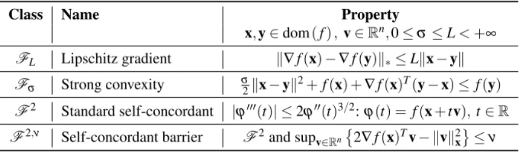
Table 1: Special convex function classes. In the optimization literature, we refer toL,σ, andνas the Lipschitz,

strong convexity, and barrier parameters, respectively.

Class Name Property

x,y∈dom(f),v∈_Rn_{,0≤σ≤L<+∞} FL Lipschitz gradient k∇f(x)−∇f(y)k∗≤Lkx−yk Fσ Strong convexity σ₂kx−yk2+f(x) +∇f(x)T(y−x)≤f(y) F2 _{Standard self-concordant |}

ϕ000(t)| ≤2ϕ00(t)3/2:ϕ(t) =f(x+tv), t∈R

F2,ν _{Self-concordant barrier} F2_{and sup} v∈Rn

2∇f(x)T_{v− kvk}2 x ≤ν

Limitation 1 (Non-ideal convergence characterizations): Ideally, the convergence characterization of an algorithm for solving (1) must establish rates both on absolute value of the primal objective residualf(xk)−f?

as well as the primal feasibility of its linear constraintskAxk−bk, simultaneously on its iteratesxk∈X. The constraint feasibility is critical so that the primal convergence rate has any significance. Rates on weighted primal objective residual and feasibility gap is not necessarily meaningful since (1) is a constrained problem and f(xk)−f?can easily be negative at all times as compared to the unconstrained setting where we trivially have f(xk)−f?≥0.

Table 2 demonstrates that the convergence results for some existing methods are far from ideal. Most algorithms have guarantees in the ergodic sense (i.e., on the averaged history of iterates without any weight) [15, 37, 38, 57, 64, 71] with non-optimal rates, which diminishes the practical performance; they rely on special function properties to improve convergence rates on the function and feasibility [56, 57], which reduces the scope of their applicability; they provide rates on dual functions [32], or a weighted primal residual and feasibility score [64], which does not necessarily imply convergence on the absolute value of the primal residual or the feasibility; or they obtain convergence rate on the gap function value sequence composed both the primal and dual variables via variational inequality and gap function characterizations [15, 37, 38], where the rate is scaled by a diameter parameter which is not necessary bounded.2

Limitation 2 (Computational inflexibility): Recent theoretical developments customize algorithms to ex-ploit special function classes for scalability. We have indeed moved away from the black-box model of opti-mization, which forms the foundation of the interior point method’s flexibility, where, for instance, we restrict ourselves to compute solely the values and the (sub)gradients of the objective and the constraints at a point.

Unfortunately, specialized algorithms requires knowledge of function class parameters, do not address the full scope of (1) (e.g., with self-concordant functions or fully non-smooth decompositions), and often have complicated algorithmic implementations with backtracking steps, which create computational bottlenecks. Moreover, these issues are further compounded by their penalty parameter selection, such asρin (2) (cf., [12] for an extended discussion), which can significantly decrease numerical efficiency, as well as the inability to handlep-decomposability in an optimal fashion, which rules out parallel architectures for their computation.

1.2

Our contributions

To this end, we address the following two questions in this paper: “Is it possible to efficiently solve (1) using only the proximal tractability assumption with global convergence guarantees?” and “Can we actually

charac-2_{We refer to the standard ADMM (see, e.g., [12]) and not the parallel ADMM variant or multi-block ADMM, which can have}

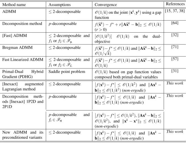
Table 2: Illustrative convergence guarantees for solving (1) under the proximal tractability assumption. Note that most convergence rate results in the table are in the ergodic oraveragedsense, where_bxk=k−1∑ki=1xi.

Method name Assumptions Convergence References

ADMM ≤2-decomposable _O(1/k)on the joint(xk_,yk_{)using a gap}

function

[15, 37, 38]

Decomposition method p-decomposable _f(_bxk_{)− f}?_+rkA

bx

k_−bk

2 ≤O(1/k)

(r>0)

[64]

[Fast] ADMM ≤ 2-decomposable and

f1or f2∈Fµ

[O(1/k2)] O(1/k) on the dual-objective

[32]

Bregman ADMM ≤2-decomposable _f(

b xk_)−f?_{≤O(1/k)andkA} b xk_−bk 2≤ O(1/√k) [71]

Fast Linearized ADMM ≤ 2-decomposable and

f1or f2∈FL f(_bxk_)−f?_{≤O(1/k)andkA} b xk_−bk 2≤ O(1/k) [57] Primal-Dual Hybrid Gradient (PDHG)

Saddle point problem O(1/k) based on gap function values composed both primal-dual variables

[31] [Inexact] augmented Lagrangian method ≤2-decomposable f(xk)−f? ≤O(1/k2) and kAxk− bk2≤O(1/k2)(non-ergodic) This work Decomposition meth-ods [Inexact] 1P2D and 2P1D p-decomposable f(xk)−f? ≤ O(1/k) and kAxk− bk2≤O(1/k)(non-ergodic) This work p-decomposable and fi∈Fσ f(xk)−f? ≤O(1/k2),kAxk−bk2≤ O(1/k2), and kxk_−x?_k 2 ≤ O(1/k) (non-ergodic) New ADMM and its

preconditioned variants ≤2-decomposable f(xk)−f? ≤ O(1/k) and kAxk− bk2≤O(1/k)(non-ergodic) This work

terize the convergence rate of the primal objective residual and primal feasibility gap separately?” The answer is indeed positive provided that there exists a solution in a bounded primal feasible setX.

Surprisingly, we can still exploit favorable function classes, such asFLandFσwhen available, optimally

exploit p-decomposability and its special 2-decomposable sub-case, and have a penalty parameter-free black-box optimization method. The second question is also important since in primal-dual framework, trade-off between the primal objective residual and the primal feasibility gap is crucial, which makes algorithm numeri-cally stable, see, e.g., [31] for numerical examples.

To achieve the desiderata, we unify primal-dual methods [10, 61], smoothing [50, 61], and the excessive gap function technique introduced in [49] in convex optimization.

Primal-dual methods: Primal-dual methods rely on strong duality in convex optimization [60] and are also related to many other methods for solving saddle points, monotone inclusions and variational inequalities [28]. In our approach, we reformulate the optimality condition of (1) as a mixed-variational inequality and use the gap function as our main tool to develop the algorithms.

Smoothing: Smoothing techniques are widely used in optimization to replace non-smooth functions with differentiable approximations. In this work, we describe two smoothing strategies for the dual function of (1) in the Lagrange formulation based on Bregman distances and the augmented Lagrangian technique. We show that the augmented Lagrangian smoother preserves convergence properties for the algorithm to solve (1) and feature a convergence rate independent of the spectral norm ofA. In addition, the Bregman smoother allows us to handlep-decomposability by only relying on the proximal tractability assumption.

Excessive gap function: Excessive gap technique was introduced by Nesterov in [49] and has been used to develop primal-dual solution methods for solving nonsmooth unconstrained problems. In this paper, we exploit the same excessive gap idea but in a structured form for a variational inequality characterizing the optimality condition of (1). We then combine these three existing techniques in order to develop a unified primal-dual framework for solving (1) and analyze the convergence of its algorithmic instances under mild assumptions.

Our specific theoretical and practical contributions are as follows:

i)We present a unified primal-dual framework for solving constrained convex optimization problems of the form (1). This framework covers augmented Lagrangian method [39, 45], (preconditioned) ADMM [15], proximal-based decomposition [20] and decomposition method [68] as special cases, which we make explicit in Section 6.

ii)We prove the convergence and establish rates for three variants (cf., Theorem 4.1) of our algorithmic framework without any need to select a penalty parameter. An important result is the convergence rate in a non-ergodic sense of both primal objective residual f(x¯k)−f?

≤O(1/kα)and the primal feasibility gap

kAx¯k_{−bk ≤O(1/k}α_{), whereα=1 or 2. Our rates are considered optimal given our particular assumptions}

(cf., Table 2).

iii)We consider an inexact variant of our algorithmic framework for the special case of 2-decomposability, which allows one to solve the subproblems up to given predetermined accuracy so that it still maintains the same worst-case analytical complexity as in the exact case provided that the accuracy of solving the subproblems is controlled appropriately. This variant allows us to handle 2-decomposability with only proximal tractability assumption.

iv)We show how special function classes can be exploited and describe their convergence implications. Our characterization is radically different from existing results such as in [5, 15, 23, 37, 38, 57, 64]. We clarify the importance of this result in Section 4 as well as Section 6 in the context of existing convergence results for ADMM and its variants. For the p-decomposability, the variants corresponding to our Bregman smoothing technique can be implemented in a fully parallel and distributed manner, where the feasibility guar-antee acts as a consensus rate. In special case, where p=2, we propose a strategy to enhance the practical convergence rate by trading off the objective residual with the feasibility gap.

On the computational front, we test our algorithms on several well-studied numerical problems using both synthetic and real-world data, compare them to other existing state-of-the-art methods, and provide open-source code for each application. We also discuss the update of the smoothness parameters in order to enhance the performance of the algorithms by trading-off between the optimality gap and the feasibility gap. Numerical results show the advantages of our methods on several numerical tests.

1.3

Related work

Due to the generality of (1), there has been an explosion of interest in the convex optimization in develop-ing solution algorithms for it. Unfortunately, it is impossible to provide a comprehensive summary of the ever-expanding literature in any reasonable space. Hence, this subsection attempts to relate some important algorithmic frameworks for solving (1) to our work with selected, representative citations in each.

Methods-of-multipliers/primal-dual methods: One of the oldest primal-dual methods for solving (1) is the method-of-multipliers (MoM), which is based on Lagrange dualization [10]. Without further assumptions on

f andX, the dual step of this method can be viewed as a subgradient iteration, which features a provably slow convergence rate, i.e.,O(1/√k), wherekis the iteration count. MoM is also known to be sensitive to the step-size selection rules for damping the search direction.

In order to overcome the difficulty of nonsmoothness in the dual function, several attempts have been made. For instance, we can add either a proximal term or an augmented term to the Lagrange function of (1) to smooth the dual function [20, 34, 35, 44, 45, 61]. Intriguingly, while the specific methods studied in [20, 34, 35, 61] are quite borad, no global convergence rate has been established so far.

The works in [44, 45] provide convergence rates by applying Nesterov’s accelerated scheme to the dual problem of (1). In recent paper [64], the authors shows that the method proposed in [20] has convergence rate

O(1/k). However, this convergence rate is a joint between the objective residual and the primal feasibility gap, i.e., f(xk_)−f?_+rkAxk_−bk

2≤O(1/k)forr>0 given. We note that this convergence rate on the weighted

measure does not imply the convergence rate off(xk)−f?

andkAxk−bk2separately in constrained

opti-mization.

In [27] the author studies several variants of the primal-dual algorithm and presented several applications in image processing. Convergence analysis of these variants are also presented in [27], however the global convergence rate has not been provided. In [31], the authors describe a primal-dual hybrid gradient (PDHG) algorithm, which can be considered as a variant of the same primal-dual algorithm. In [31], the authors also studied several heuristic strategies to update the parameters, and show that the convergence rate of this algo-rithm isO(1/k)in an ergodic sense with respect to a VIP gap function values.

Methods from monotone inclusions and variational inequalities: The optimality condition of (1) can be viewed as a monotone inclusion or a mixed variational inequality (VIP) corresponding to both the primal and dual variables[x,y]∈X ×_Rm_{. As a result, we can leverage algorithms from these two respective fields to}

solve (1) [15, 28, 37, 38]. For instance, the work in [15] exploit the idea from variational inequality proposed in [47, 51]. Splitting methods including Douglas-Rachford and predictor-corrector methods considered [21, 22, 26, 36, 55] also belong to this direction. However, since monotone inclusions or variational inequalities are much more general than (1), using methods tailored for optimization purposes may be more efficient in practice for solving the specific optimization problem (1).

Augmented Lagrangian and alternating direction methods: Augmented Lagrangian (AL) methods have come to offer an important computational perspective on a broad class of constrained convex problems of the form (1). In this setting, we first define the Lagrangian function associated with the linear constraint

Ax=bof (1) as L(x,y):= f(x) +yT(Ax−b). Then, we introduce the augmented Lagrangian function:

Lγ(x,y):=L(x,y) + (γ/2)kAx−bk2₂for a given penalty parameterγ>0. Classical augmented Lagrangian

method [11] solving (1) produces a sequence(xk_,yk₎

k≥0starting from(x 0_,y0_{)∈X ×} Rmas xk+1 _{:=arg min} x∈X Lγ(x,yk), yk+1 :=yk+γ(Axk+1−b), (5)

Under a suitable choice ofγ, it is well-known that method (5) converges to a global optimal(x?,y?)of (1) atO(1/k)rate under mild assumptions, i.e., L(xk_,yk_)−L(x?_,y?_{)≤O(1/k). In fact, this method can be}

accelerated by applying Nesterov’s accelerating scheme [48] to obtainO(1/k2)convergence rate.

Within the class of augmented Lagrangian methods, perhaps the most famous variant is the alternating direction method of multipliers (ADMM), which appears in many guises in the literature. This method has been recognized as a special case of Douglas-Rachford splitting algorithm applying to its optimality condition [12, 26, 32]. In ADMM, given that f andX are separable withp=2. This case also covers the composite minimization problem of the form min_x1∈Rn1 f1(x1) +f2(Ax1), where both f1and f2 are convex. By using

Ax1=x2. In the ADMM context, the first problem in (5) can be solved iteratively as      xk₁+1 :=arg min x1∈X1 n f1(x1) + (yk)TA1x1+ (γ/2)kA1x1−xk2k22 o , xk₂+1 :=arg min x2∈X2 n f2(x2) + (yk)TA2x2+ (γ/2)kA1xk1+1−x2k22 o . (6)

The main computational difficulty of ADMM is thex1-update problem (i.e., the first subproblem) in (6).

In-deed, we have to numerically solve this step in general except whenATAis efficiently diagonalizable. Inter-estingly, the diagonalization step in many cases can be done via Fourier Transform. Many notable applications support this feature, such as matrix completion whereAmodels sub-sampled matrix entries, image deblurring whereAis a convolution operator, and total variation regularization whereAis a differential operator with periodic boundary conditions. We can also circumvent this computational difficulty by using a preconditioned ADMM variant [15].

ADMM is one of the most popular method in practice. However, its efficiency depends significantly on the choice of the penalty parameterγ. Unfortunately, theoretical guarantee for choosing this parameter is still an open problem and is not yet well-understood. When f1is strongly convex, we can drop the quadratic term in the first line of (6) in order to obtain an alternating minimization algorithm (AMA) [69]. This method turns out to be a forward-backward splitting algorithm for its optimality inclusion [32].

A note on [50]: We note that the approach presented in this paper builds upon the excessive gap idea in [50]. Technically, we use the same idea but in a much structured fashion, whereby we enforce a particular linear form in preserving the excessive gap as shown in Definition 3.2. This particular structure is key in obtaining our convergence rates.

Moreover, since our problem setting (1) is different from the general minmax formulation considered in [49], there are still several differences between our algorithmic framework and the methods studied in [49] as a result of the excessive gap technique. First, we use augmented Lagrangian functions and Bregman distances for smoothing the dual problem of (1). Second, we consider the Lagrangian primal-dual formulation for (1) where we do not have the boundedness of the feasible set of the dual variable. In this case the key estimate [50, estimate (3.3)] does not apply to our setting. Third, we update all algorithmic parameters simultaneously and do not need an odd-even switching strategy [49, Method 1: b) and c)]. Four, we do not assume that the objective function fof (1) has Lipschitz gradient which is required in [49]. Note that there are several important applications, where this assumption simply does not hold [43]. Fifth, our method is applied to the constrained problem (1), which requires the feasibility gap characterization as opposed to unconstrained problems where we only need to worry about the primal-dual optimality.

1.4

Paper organization

The rest of this paper is organized as follows. In the next section, we recall basic concepts, and introduce a mixed-variational inequality formulation of (1). In Section 3, we propose two key smoothing techniques for (1), called the Bregman and augmented Lagrangian smoothing techniques. We also provide a formal definition for the excessive gap function from [50] and further investigate its properties. Section 4 presents the main primal-dual algorithmic framework for solving (1) and its convergence theory. Section 5 specifies different instances of our algorithmic framework for (1) under given assumptions. Section 6 makes further connections to existing methods in the literature. Section 7 is devoted to implementation issues and Section 8 presents numerical simulations. The appendix provides detail proofs of the theoretical results in the main text.

2

Preliminaries

First we recall the well-known definition of the Bregman distance, the primal-dual formulation for (1), and a variational inequality characterization for the optimality condition of (1), which will be used in the sequel.

2.1

Basic notation

Given a proper, closed and convex function f, we denote dom(f):={x∈Rn| f(x)<+∞}the domain of f,

∂f(x):={v∈Rn| f(x˜)−f(x)≥vT(x˜−x), ∀x˜∈dom(f)}the subdifferential of f atx. If f is differentiable,

∇f(x)denotes the gradient of f atx. For given vectorx∈Rn, we definekxk2the Euclidean norm ofx. We

use a superscripted notationLf >0 to denote the corresponding Lipschitz constant of a differentiable function

f. Similarly, we use a subscripted notationσg>0 to denote the corresponding strong convexity constant of a

convex functiong.

2.2

Proximity functions and Bregman distances

Given a nonempty, closed convex set X, a nonnegative, continuous and σb-strongly convex function b is

called aproximityfunction (or prox-function) ofX ifX ⊆dom(b). For example, the simplest prox-function isb_X(x):= (σb/2)kx−xck22for anyσb>0 andxc∈X. Whenever unspecified, we use this specific

prox-function withσb=1.

Given a smooth prox-functionbofX with the parameterσb>0. We define

db(x,y):=b(x)−b(y)−∇b(y)T(x−y), ∀x,y∈dom(b), (7)

the Bregman distance between x andy with respect tob. Given a matrixS, we also define the projected prox-diameter of a given setX with respect todbas

DS_X := sup

x,xc∈X

db(Sx,Sxc). (8)

Here, we project the setX onto the range space of matrixS. IfX is bounded, then 0≤DS_X <+∞. For

b(x):= (σb/2)kx−xck22, we havedb(x,y) = (σb/2)kx−yk22, which is indeed the Euclidean distance.

2.3

Primal-dual formulation

We write the min-max formulation of (1) based on the Lagrange dualization as follows: max y∈Rm min x∈XL(x,y)≡ymax∈Rm min x∈X{f(x) +y T_{(Ax−b)}, (9)}

whereL is the Lagrange function andyis the dual variable. We write the dual functiong(y)as

g(y):=min

x∈X{f(x) +y

T_{(Ax−b)}, (10)}

which leads to the following definition of the so-called dual problem

g?:=max

y∈_Rmg(y). (11)

Letx?(y)be a solution of (10) at a giveny∈Rm. Corresponding tox?(y), we also define the domain ofgas

If f is continuous onX and if X is compact, then x?(y)exists for any y∈Rm. Unfortunately, the dual

function g is typically nonsmooth, and hence the numerical solutions of (11) are usually difficult [48]. In general, we haveg(y)≤f(x), which is known as weak-duality in convex optimization. In order to guarantee strong duality, i.e., f?=g?for (1) and (11), we require the following assumption:

Assumption A. 1 The constraint setX and the solution setX?of(1)are nonempty. The function f is proper, closed and convex. In addition, eitherX is a polytope or the following Slater condition holds:

{x∈_Rn_{|Ax=b} ∩relint(X)6=/0, (13)}

whererelint(X)is the relative interior ofX.

Under Assumption 1, the solution setY?of the dual problem (11) is also nonempty and bounded. More-over, the strong duality holds, i.e., f?=g?. Any point(x?,y?)∈X?_×Y?_{is a primal-dual solution to (1)}

and (11), and is also a saddle point of the Lagrange functionL, i.e.,L(x?,y)≤L(x?,y?)≤L(x,y?)for all

x∈X andy∈Rm. These inequalities lead to the following estimate

f(x)−g(y)≥f(x)−f?≥ −ky?k2kAx−bk2, ∀x∈X,y∈Rm. (14)

Our goal in this paper is to solve the primal constrained problem (1), while numerical algorithms only give an approximate solution up to a certain accuracy. Hence, we need to specify the concept of an approximate solution for (1).

Definition 2.1 Given a target accuracyε≥0, a pointx˜?_{∈X is said to be anε-solution of(1)if|f(x˜}?_)−f?_{| ≤} εandkAx˜?_−bk

2≤ε.

Here, we assume in Definition 2.1 that ˜x?∈X, i.e., ˜x?is exactly feasible toX. This requirement is reasonable in practice sinceX is usually a “simple” set where the projection ontoX can be computed exactly. Moreover, we can use different accuracy levels for the absolute value of the primal objective residual|f(x˜?)−f?|and the primal feasibility gapkAx˜?−bk2in Definition 2.1.

2.4

Mixed-variational inequality formulation and gap function

Letw:= (x,y)≡(xT,yT)T∈Rn×Rmbe the primal-dual variable andF(w):=

ATy b−Ax

be a partial Karush-Kuhn-Tucker mapping. Then, the optimality condition of (1) becomes

f(x)−f(x?) +F(w?)T(w−w?)≥0, ∀w∈X ×Rm, (15)

which is known as amixed-variational inequality[28]. If we define

G(w?):= max

w∈W:=X×Rm

f(x?)−f(x) +F(w?)T(w?−w) , (16) thenGis known as the Auslender gap function of (15) [1].

LetW :=X ×Rm. Then, by the definition ofF, we can see that G(w?) = max

(x,y)∈W

f(x?) +yT(Ax?−b)−f(x)−(Ax−b)Ty? =f(x?)−g(y?)≥0.

It is clear thatG(w?_{) =0 if and only ifw}?_{:= (x}?_,y?_)∈W?_:=X?_×Y?_{, which is indeed thestrong duality}

3

Primal-dual smoothing techniques

This section shows how to use augmented Lagrangian functions and Bregman distances as a principled smooth-ing technique [48, 3] within our primal-dual framework. We can then obtain different algorithmic variants by simply choosing an appropriate prox-center at each iteration.

3.1

Dual function is a smoothable function

The dual functiongdefined by (10) is convex but in general nonsmooth. We approximate this function by a smoothed functiongγdefined as:

gγ(y):=min

x∈X

f(x) +yT(Ax−b) +γdb(Sx,Sxc) , (17)

wheredbis a given Bregman distance with the strong convexity parameterσd>0,xc∈X is the prox-center

ofdb,Sis a given consistent projection matrix andγ>0 is a [primal]smoothnessparameter. The following

definition characterizes approximation properties of the smoothed functiongγ.

Definition 3.1 ([3]) The dual function g defined by(10)is called a(γ,D,L¯g)-smoothable function if there exist positive numbersγ, D andL¯gand a concave and smooth function gγ: dom(g)→R∪ {+∞}so that:

gγ(y)−γD≤g(y)≤gγ(y), ∀y∈dom(g). (18)

In addition,∇gγ(·)is Lipschitz continuous with a Lipschitz constant L g γ:=γ

−1_L¯g_.

We callgγthe(γ,D,L¯g)-smoothed function ofgor simply the smoothed function ofgwhen these parameters

are specified. We note thatgγdefined by (17) is not necessarily Lipschitz gradient for an arbitrary choice ofS

andx_c. We consider two cases as follows.

3.1.1 Smoothing via augmented Lagrangian

Let us choose db(u,uc):= (1/2)ku−uck22, S≡A andxc∈X so that Axc=b. Then, we have trivially

db(Sx,Sxc):= (1/2)kAx−bk22. As a result, the functiongγ defined by (17) becomes the augmented dual

function, that is ˜ gγ(y):=min x∈X f(x) +yT(Ax−b) + (γ/2)kAx−bk2₂ . (19)

Here,Lγ(x,y):=f(x) +yT(Ax−b) + (γ/2)kAx−bk2₂is exactly the augmented Lagrangian of (1) associated

with the linear constraintAx=b. We denote by ˜x?

γ(y)the solution of (19) and dom ˜gγ

:=

y∈Rm|x˜?γ(y)exists .

It is well-known that ˜gγis concave as well as smooth, and its gradient is Lipschitz continuous with a Lipschitz

constantLgγ˜:=γ−1. We refer to ˜gγ as an augmented Lagrangian smoother (in short,AL smoother) ofg. The

following lemma shows that ˜gγis a smoothed function ofg, whose proof can be found, e.g., in [10].

Lemma 3.1 For any γ>0,g˜γ defined by (19)is concave and smooth. Its gradient is given by ∇g˜γ(y) =

Ax˜?_γ(y)−band satisfies: k∇g˜γ(y)−∇g˜γ(yˆ)k2≤Lgγ˜ky−yˆk2, ∀y,yˆ∈dom ˜gγ , (20) where Lgγ˜:=γ −1_>0.

Consequently,g˜γis a (γ,DA_X,L¯g˜)-smoothed function of g in the sense of Definition 3.1, i.e.,g˜γ(y)−γDA_X ≤

3.1.2 Smoothing via Bregman distances

If we chooseS:=Ito be the identity matrix ofRn, then the smoothed functiongγdefined by (17) becomes

ˆ gγ(y):=min x∈X f(x) +yT(Ax−b) +γdb(x,xc) . (21) Let us denote by ˆx?

γ(y)the solution of (21), which always exists. We refer to ˆgγas a Bregman distance smoother

(shortly,BD smoother) ofg. The following lemma summarizes the properties of ˆgγ(see, e.g., [50, 68]):

Lemma 3.2 The functiongˆγdefined by(21)satisfies:

ˆ

gγ(y)−γDIX ≤gˆγ(y)−γdb(x?(y),xc)≤g(y)≤gγ(y), ∀y∈R

m_{, (22)}

where DI

X is the prox-diameter ofX with respect to dbandx?(y)is the solution of (10).

Moreover,gˆγ is concave and smooth. Its gradient is given by∇gˆγ(y):=Axˆ?γ(y)−bfor ally∈R m_{, and} satisfies ∇gˆγ(y)−∇gˆγ(yˆ) 2≤L ˆ g γky−yˆk2, ∀y,yˆ∈Rm, (23) for Lgγˆ:= kAk2 2 γ σd . Consequently, gˆγ is a(γ,D I

X,L¯gˆ)-smoothed function of g, whereL¯gˆ:= kAk2

2

σd and σd is the

strong convexity parameter of db.

We note that ifX is bounded and f is continuous (orX ⊂relint(dom(f))), thenx?_{(y)always exists for}

anyy∈_Rm_{. In this case, the prox-diameterD}I

X ofX is finite. Consequently, (22) holds for ally∈Rm.

3.2

Smoothed gap function

As we observe from the previous section, the optimality condition of (1) can be represented as a variational inequality of the form (15). By using Auslender’s gap functionG(·)defined by (16), we can show thatw?∈W?

is a primal-dual solution to (1) and (11). Since the gap functionG(·)is generally nonsmooth, we smooth it by adding the following smoothing function:

dγ β(w)≡dγ β(x,y):=γdb(Sx,Sxc) + (β/2)kyk22, (24)

where db is a given Bregman distance, S is a projection matrix andγ and β are two positivesmoothness

parameters.

Remark 3.1 For simplicity of our analysis, we use a simple quadratic prox-function(β/2)kyk2

2in(24)for the dual variabley. However, we can replace this term byβdby(y,yc), where dby is a given Bregman distance and

y_cis a given point inRm. However, depending on the choice of dby, the dual variabley∗β(·)may no longer have

a closed form expression. However, the overall practical performance may be improved.

The smoothed gap function forGis then defined as follows:

Gγ β(w¯):= max

w∈X×Rm

f(x¯)−f(x) +F(w¯)T(w¯−w)−dγ β(w) , (25)

whereFis defined in (15). The functionGγ βcan be considered as Fukushima’s gap function [29] for the

vari-ational inequality problem (15). We can see thatGγ β(w¯)→G00(w¯)≡G(w¯)asγandβ→0+simultaneously.

It is clear that the maximization problem (25) is a convex optimization problem. We denote byw?

γ β(w¯):= (x?_γ(y¯),y?

β(x¯))the solution of this problem. Then, by using the optimality condition of (25) we can easily check

thatx?_γ(y¯)is the optimal solution to (17) aty:=y¯, whiley?

β(x¯)can be computed explicitly as

y?_β(x¯):=β−1(Ax¯−b). (26) Our goal is to generate two sequencesw¯k _k≥0⊆W and{(γk,βk)}k≥0∈R2++so that

Gγkβk(w¯ k₎

k≥0becomes

Definition 3.2 (Model-based Excessive Gap) Givenw¯k:= (x¯k,y¯k)∈W and(γk,βk)>0, a new pointw¯k+1:= (x¯k+1,y¯k+1)∈W and (γk+1,βk+1)>0 so thatγk+1βk+1<γkβk is said to be firmly contractive(w.r.t. Gγ β

defined by(25))if:

Gk+1(w¯k+1)≤(1−τk)Gk(w¯k)−ψk, (27)

where Gk(·):=Gγkβk(·),τk∈[0,1)andψk∈Rare two given parameters.

Here, the parameterτkand the decay termψkwill be specified accordantly with different algorithmic schemes.

In the context of excessive gap technique introduced by Nesterov, the smoothed gap functionGµ1µ2(w¯)

measures the excessive gap fµ2(x¯)−φµ1(y¯)in [49, cf., (2.5) and (2.9)]). Hence, we will callGγ β(w¯)Nesterov’s

smoothed gap function customized for the constrained convex problem (1). We note that the excessive gap condition fµ2(x¯)≤φµ1(y¯)in [49, (3.2)] only requiresGµ1µ2(w¯)≤0. In our case, we structure this condition

using the basic model in (27) so that we can manipulateτkand the new parameterψksimultaneously to analyze

the convergence of our algorithms.

In the sequel, we often assume that the second parameterψkis nonnegative, which allows us to estimate the

convergence rate of

Gk(w¯k) _k≥0. However, the following remark shows that the sequenceGk(w¯k) _k≥0can

still converge to 0+even ifψkis positive. However, we find the ensuing convergence analysis to be difficult.

Remark 3.2 Let{τk}k≥0⊆(0,1)and{ψk}k≥0be sequences in Definition 3.2. If

lim k→∞ τk=0, ∞

∑

∑

then the sequenceGk(w¯k) _k≥0converges to0

+_.

From Definition 3.2, ifw¯k _k≥0⊆W and{(γk,βk)}k≥0∈R2++satisfy the condition (27), then we have

Gk(w¯k)≤ωkG0(w¯0)−Ψkby induction, where ωk:= k−1

∏

∑

∏

Consequently, the rate of convergence of

Gk(w¯k) _k≥0depends on the rate of{τk}k≥0and{ψk}k≥0.

The next lemma shows the relation between problem (1) and its smoothed functiongγandg. The proof of

this lemma can be found in the appendix.

Lemma 3.3 Let gγ be defined by(17)and Gγ β defined by(25). Also, let

¯

wk

k≥0⊂W and{(γk,βk)}k≥0∈ R2++be the sequences satisfying Definition 3.2. Then we have

f(x¯k)−gγk(y¯

k_)≤

ωkG0(w¯0)−Ψk−(1/(2βk))kAx¯k−bk22. (30) In addition, we also have the following bound:

−ky?k2kAx¯k−bk2≤f(x¯k)−f?≤ f(x¯k)−g(y¯k)≤Sk, (31) kAx¯k−bk2≤βk h ky?k2+ q ky?_k2 2+2β −1 k Sk i (32)

where Sk:=ωkG0(w¯0) +γkDS_X −Ψk, provided thatβkky?k22+2Sk≥0.

From Lemma 3.3 we can see that ifG0(w¯0)≤Ψk, then the primal objective residual

f(x¯k)−f? and the

primal feasibility gapkAx¯k_−bk

2of (1) are bounded by    f(x¯k)−f? ≤max n γkDS_X, 2βkDY?+ q 2γkβkDS_X D_Y? o , kAx¯k_−bk 2≤2βkDY?+ q 2γkβkDS_X, (33)

whereD_Y?:=min{ky?k₂|y?∈Y?}, which is the norm of a minimum norm dual solution. The estimate (33)

hints that we can derive algorithms based on{(γk,βk)}whose convergence rate depends directly on how we

update the sequence{(γk,βk)}k≥0.

4

The main algorithmic framework

The key objective in this section is to design a primal-dual update template from ¯wk∈W and(γk,βk)∈R2++

to ¯wk+1_{∈W and(γ}

k+1,βk+1)∈R2++so that the conditions in Definition 3.2 hold. We develop two distinct

schemes to update ¯wk_and(γ

k,βk)in the following two subsections.

4.1

An iteration scheme with two primal steps

Since the objective function is not necessary smooth, we consider the following mapping under Assumption 1: prox_Sf(x,ˆ yˆ;β):=arg min

x∈X

f(x) +yˆTA(x−xˆ) + (L¯g/(2β))kS(x−xˆ)k2₂ , (34)

whereβ>0 andSis a projection matrix that satisfies the following condition:

kAx−bk2₂≤ kAxˆ−bk2₂+2(Axˆ−b)TA(x−xˆ) +L¯gkS(x−xˆ)k2₂, ∀x,xˆ∈X. (35) An obvious choice ofS is eitherS≡Aand ¯Lg=1 or S≡Iand ¯Lg=kAk22. Since Ais known, both are

feasible. Alternatively, local variable metrics can be used here, which might lead to different adaptation and computation tradeoffs in optimization.

Now, given ¯wk_{:= (x¯}k_,y¯k_{)∈W and(γ}

k,βk)∈R2++, we computex?γ(y¯

k_{)the solution of the minimization}

problem in (17) andy?

β(x¯

k_{)by (26). Then, we update the point ¯w}k+1_{:= (x¯}k+1_,y¯k+1_)and(

γk+1,βk+1)based on

the following scheme:

       ˆ xk := (1−τk)x¯k+τkx?γk(y¯ k_), ˆ yk _:=β−1 k+1(Axˆk−b), ¯ xk+1 _:=prox Sf(xˆk,yˆk;βk+1), ¯ yk+1 _{:= (1−τ} k)y¯k+τkyˆk, (2P1D)

whereτk∈(0,1]and(βk+1,γk+1)is updated as

βk+1= (1−τk)βk and γk+1= (1−ckτk)γk, (36)

for some ck∈(−1,1], which will be specified later. It is important to note that if f is nonsmooth, solving

problem (34) requires the same cost as solving (17). Therefore, we can refer to (2P1D) as a primal-dual scheme with two primal steps.

Remark 4.1 If f is Lf-Lipschitz gradient, then we can replace f(x)in the proximal step at the third line of

(2P1D)by its linearization, which leads to the following gradient step:

grad_Sf(x,ˆ yˆ;β):=argmin x∈X (∇f(xˆ) +ATy)T(x−xˆ)+(Lf/2)kx−xˆk22+(2β) −1_kS(x−xˆ)k2 2 .

In particular, when f is p-decomposable as in(3)and if fiis Lipschitz gradient for some i=1, . . . ,p, then we

can use the gradient step for such a fi[68].

The following lemma provides conditions such that(x¯k+1_,y¯k+1_{)updated by (2P1D) satisfies Definition 3.2,}

Lemma 4.1 Let (x¯k+1,y¯k+1)and (γk+1,βk+1)be updated as(2P1D)and (36). IfS satisfies(35) andτk is

chosen such that

βk+1γk+1≥L¯gτk2, (37)

then(x¯k+1,y¯k+1)∈W and satisfies Definition 3.2, i.e., Gk+1(w¯k+1)≤(1−τk)Gk(w¯k)−ψkforψk:= τ_k2 2βk+1kAx ? γk(y¯ k₎₋ bk2 2≥0.

4.2

An iteration scheme with two dual steps

Alternatively to (2P1D), we can switch from two primal steps to two dual steps. In this case, the new point

(x¯k+1_,y¯k+1_{)is updated as follows:}      ˆ yk := (1−τk)y¯k+τky?_β k(x¯ k_), ¯ xk+1 _{:= (1−τ} k)x¯k+τkx?γk+1(yˆ k_), ¯ yk+1 _:=yˆk₊γk+1 ¯ Lg Ax?γk+1(yˆ k_)−b , (1P2D)

whereτk∈(0,1)and the parametersβk+1andγk+1are updated as (36). We refer to (1P2D) as aprimal-dual scheme with two dual steps.

The following lemma shows that(x¯k+1,y¯k+1)updated by (1P2D) maintains (27), whose proof can also be found in the appendix.

Lemma 4.2 Let(x¯k+1,y¯k+1)and(γk+1,βk+1)be updated by(1P2D)and(36), respectively. Ifτk is chosen

such that

βk+1γk+1≥L¯gτk2, (38)

then(x¯k+1_,y¯k+1_{)∈W and satisfies G}

k+1(w¯k+1)≤(1−τk)Gk(w¯k)−ψkfor ψk:=τk(1−τk)γk db(Sx?γk+1(yˆ k_),Sx c)−ckdb(Sx?γk+1(y¯ k_),Sx c)≥0.

4.3

Finding a starting point

In principle, we can start our algorithm at any point(x¯0,y¯0)∈W. However, we can find a point ¯w0:= (x¯0,y¯0)∈ W such thatG_γ0β0(w¯0)≤0. The following lemma shows how to compute such a point, whose proof can be found in the appendix.

Lemma 4.3 Givenx0_c∈X, the pointw¯0:= (x¯0,y¯0)∈W computed by

¯ x0=x?_γ 0(0 m_), ¯ y0_:=β−1 0 Ax¯0−b . (39) satisfies G_γ 0β0(w¯ 0_{)≤ −} γ0db(Sx¯0,Sxc)≤0provided thatβ0γ0≥L¯g. Alternatively, the pointw¯0:= (x¯0,y¯0)∈W generated by

¯ y0 :=β₀−1(Axc−b), ¯ x0 :=prox_Sf(xc,y¯0;β0), (40) also satisfies Gγ0β0(w¯ 0_{)≤ −γ0d} b(Sx¯0,Sxc)≤0provided thatβ0γ0≥L¯g.

4.4

Updating step-size parameter

It remains to derive an update rule for the step-sizeτkin both scheme (2P1D) and (1P2D). The update rule is

derived by using the same condition in both Lemma 4.1 and Lemma 4.2.

Since τk satisfies βk+1γk+1≥L¯gτk2, τk+1 also satisfies the same condition, i.e., βk+2γk+2≥L¯gτk2+1. In

addition, by (36), we haveβk+2:= (1−τk+1)βk+1andγk+2:= (1−ck+1τk+1)γk+1. These conditions lead to τ_k2₊₁≤(1−τk+1)(1−ck+1τk+1)τk2. Since we want to maximize the value ofτk+1, we take the equality, i.e., τ_k2₊₁= (1−τk+1)(1−ck+1τk+1)τk2. The last condition leads to

ak+1:= 1+ck+1+

q

4a2_k+ (1−ck+1)2

/2, and τk:=a−k1. (41)

In addition, from Lemma 4.3, we haveβ0γ0≥L¯g. Let us chooseβ0:=γ₀−1L¯g. We need to chooseτ0∈(0,1]

such thatγ1β1= (1−τ0)(1−c0τ0)β0γ0≥L¯gτ₀2. Therefore, we get

a0:=1+c0+

q

4(1−c0) + (1+c0)2_{/2, andτ0:=a}−1

0 . (42)

The following Lemma shows the convergence rate ofak,βkandβkγk. The proof of this lemma can be found in

the appendix.

Lemma 4.4 Let sk:=∑ki=1ci. Then, the sequence{ak}updated by(41)with a0given by(42)satisfies

(k+a0+sk)/2≤ak≤k+a0. (43)

Consequently, the sequences{βk}and{γk}updated by(36)satisfy

¯ Lg (k+a0)2≤γk+1βk+1≤ 4 ¯Lg (k+a0+sk)2 , (44)

whereL¯gis given in Definition 3.1. Moreover, we also have

( _β

0

(k+2)2 ≤ βk+1 ≤_(k4₊β₁0₎2, if ck=0,

βk+1 =kβ+02, if ck=1.

(45)

4.5

A primal-dual algorithmic template

Now, we combine all ingredients presented in the previous subsection to obtain the template for solving (1) shown in Algorithm 1.

The main step of Algorithm 1 is Step 5, where we need to update(x¯k+1,y¯k+1)based on either (2P1D) or (1P2D). If we use (2P1D), thenγkcan be updated asγk+1:= (1−τk)γk, i.e.,ck=1. We can also fixγk=γ0>0

for all the iterationsk≥0, i.e.,ck=0. It is important to note that Step 5 and Step 6 are mixed. Depending

on the use of either (2P1D) or (1P2D), the corresponding parameterβkorγkis updated before Step 5. If we

chooseck<0, then{γk}is increasing. Since the rate ofβkγkis fixed atO(1/k2)due to (44), if we decrease the

rate of{γk}(i.e., increaseγk), then{βk}converges faster than theO(1/k2)rate. We will discuss the stopping

condition at Step 4 later. We note that we can also alternate between (2P1D) and (1P2D) in Algorithm 1. However, it is not clear whether this strategy would yield any numerical advantage.

4.6

Convergence analysis

Under Assumption 1, the dual solution setY?is nonempty. Recall thatD_Y?:= min

y?_∈Y?ky

?_k

2<+∞is the norm

Algorithm 1:(Primal-dual template using model-based excessive gap technique)

Inputs:γ0>0,c0∈(−1,1], and a smoother (AL or BD).

Initialization:

1: a0:= 1+c0+ [4(1−c0) + (1+c0)2]1/2/2 andτ0:=a−₀1. 2: Use ¯Lg:=1 for AL smoother and ¯Lg:=σ_d−1kAk2₂for BD smoother.

3: β0:=L¯g/γ0.

4: Compute(x¯0_,y¯0_{)by either (39) or (40).}

Fork=0tokmax

5: Ifstopping criterion, terminate.

6: Given(x¯k,y¯k), update(x¯k+1,y¯k+1)by either (2P1D) or (1P2D).

7: βk+1:= (1−τk)βkand updateγk+1:= (1−ckτk)γk.

8: Updateck+1fromckif necessary.

9: Updateak+1:= 1+ck+1+ [4a2k+ (1−ck+1)2]1/2

/2 and setτk+1:=a−_k+11.

End For

Theorem 4.1 Let (x¯k,y¯k) _k≥0be the sequence generated by Algorithm 1 after k≥1 iterations. Then, if gγ≡g˜γ, i.e., using augmented Lagrangian smootherg˜γ, then:

a) If ck:=0for all k≥0,γ0:=L¯g˜=1, then:

( kAx¯k−bk2≤ 8DY ? (k+1)2, −1 2kAx¯ k_−bk2 2−DY?kAx¯k−bk2≤ f(x¯k)−f?≤ 0, (46)

for all k≥0. Moreover, the spectral norm ofAdoes not affect the bounds in(46).

As a consequence, the worst-case analytical complexity of Algorithm 1 to achieve anε-primal solutionx¯kfor

(1)in the sense of Definition 2.1 isO ε−1/2.

Alternatively, if gγ≡gˆγ, i.e., using Bregman distance smootherg˜γ, then:

b) If Algorithm 1 uses(2P1D),γ0:=

√

¯

Lg_{and c}

k:=1for all k≥0, then:

   kAx¯k_−bk 2 ≤ √ ¯ Lg_2D Y?+q2DI X k+1 , −D_Y?kAx¯k−bk₂≤ f(x¯k)−f? ≤ √ ¯ Lg k+1DIX. (47) c) If Algorithm 1 uses(1P2D),γ0:=2 √ 2 ¯Lg

K+1 and ck:=0for all k=0, . . . ,K, then:

   kAx¯K_−bk 2 ≤ 2√2 ¯Lg(D_Y?+ q DI X) (K+1) , −D_Y?kAx¯K−bk₂≤ f(x¯K)−f? ≤2 √ 2 ¯Lg (K+1)DIX. (48)

As a consequence, the worst-case analytical complexity of Algorithm 1 to achieve anε-primal solutionx¯k_for

(1)in the sense of Definition 2.1 isO ε−1.

We note that the choice ofγ0in Theorem 4.1 trades-off the primal objective residual and the primal

feasi-bility gap. Indeed, smallerγ0leads to smaller|f(x¯k)−f?|.

We chose the(1P2D)scheme above due to its close relationship to some well-known primal dual methods we describe below. Unfortunately, the(1P2D)scheme has the drawback of fixing the total number of iterations

5

Instances of Algorithm 1

This section specifies Algorithm 1 under different assumptions to obtain specific instances of this algorithm for solving (1).

5.1

Strong convexity assumption

If the objective function f of (1) is strongly convex with a convexity parameterσf >0. Then it is well-known

that (see, e.g., [50]) the dual functiong(·)defined by (10) is smooth and Lipschitz gradient with a Lipschitz constantLg_f :=kAk22

σf . In this case, we modify accordingly both schemes (2P1D) and (1P2D) as follows:

(2P1Dσ)    ˆ xk _{:= (1−τ} k)x¯k+τkx?(y¯k), ¯ xk+1 _:=prox If(xˆk,β −1 k (Axˆk−b);βk), ¯ yk+1 _{:= (1−τ} k)y¯k+βτkk Axˆ k_−b . (1P2Dσ)      ˆ yk _{:= (1−τ} k)y¯k+τky?βk(x¯ k_), ¯ xk+1 := (1−τk)x¯k+τkx?(yˆk), ¯ yk+1 :=yˆk+1 Lg_f Ax ?_(yˆk_)−b .

While the scheme(1P2Dσ)remains similarly to (1P2D), the parameterβkin(2P1Dσ)has not updated yet as

in (2P1D).

The starting point ¯w0:= (x?(0m),y¯0)∈W for Algorithm 1 with respect to this variant can be computed as ¯

y0:= (Lg_f)−1(Ax?(0m)−b)andx?(y)is the unique solution of the minimization in (10). The parametersβk

andτkare updated as follows:

βk+1:= (1−τk)βk, τk+1:= (τk/2)[(τk2+4)1/2−τk], k≥0, (49)

whereβ0:=Lg_f andτ0:= (

√

5−1)/2. The following corollary shows the convergence of both schemes, whose proof is in the appendix.

Corollary 5.1 Assume that f of (1)isσf-strongly convex. Let(x¯k,y¯k) _k≥0be a sequence generated by either (2P1Dσ)or(1P2Dσ)using the update rule(49). Then

       kAx¯k−bk2≤ 4kAk2 2 (k+2)2_σ fDY ?, −D_Y?kAx¯k−bk₂≤ f(x¯k)−f?≤ 0, kx¯k_−x?_k 2≤ _(k4₊kA₂₎k_σ2 fDY?, (50)

where D_Y? is defined in Theorem 4.1 andx?∈X?.

As a consequence, the worst-case analytical complexity for finding anε-primal solutionx¯kof (1)in the sense of Definition 2.1 isO(1/√ε).

Remark 5.1 The bounds in(50)do not depend on the prox-diameter DI

X of the feasible setX. Hence, the

boundedness ofX is no longer required.

Remark 5.2 Convergence of the objective indeed depends on the absolute value of the primal residual, i.e.,

|f(x¯k_)−f?_{| ≤} 4kAk2 2 (k+2)2_σ fD 2 Y?.

5.2

Lipschitz gradient assumption

The aim of this subsection is to develop a variant of Algorithm 1 using (1P2D) without fixed the accuracy as stated in Theorem 4.1(c). However, this variant is only limited to problems of the form (1) that satisfy the following technical assumption:

Assumption A. 2 The following conditions hold:

(a) The objective function f and the feasible setX of (1)are separable as in(3).

(b) The last term fp is Lfp-Lipschitz gradient and the smallest eigenvalue λmin(ATpAp) of matrixAp is

positive.

(c) The Bregman distance d(Sx,Sx_c) is chosen as d(Sx,Sx_c):=∑_ip₌₁di(Sixi,Sixci), where Sp ≡I and dp(·,xcp)is smooth and∇dp(·,xcp)is1-Lipschitz continuous.

(d) The last term gγpof the smoothed dual function gγdefined by(17)satisfies

gγp(y) = min

xp∈Rnp

fp(xp) +yTApxp+ (γ/2)dp(xp,xcp) . (51)

That is the primal constraint on the last component is not active.

Under Assumption A.2, we can write the functiongγdefined by (17) asgγ(y):=∑ p i=1giγ(y)−b T_{y, where} gi_γ(y):= min xi∈Xi fi(xi) +yTAixi+ (γ/2)di(Sixi,Sixic) , i=1, . . . ,p.

A simple example fordpisdp(xp):= (1/2)kxp−xcpk22. The last condition in Assumption A.2 shows that the

solutionx?_p,γ(y)of the minimization problem ingγpmust be attained in relint(Xp). This condition is not too

restrictive, since we only require it for the last componentgpγ. It is automatically fulfilled if fp is strongly

convex andxc_p∈relint(Xp). Now, we show that the functiongpγ is strongly concave in the following lemma,

whose proof can be found in the appendix.

Lemma 5.1 Under Assumption A.2, the function gγpdefined by(51)is strongly concave with the parameter

σ_gp

γ := (Lfp+γ) −1

λmin(AT_pAp)>0. Consequently, the function gγdefined by(17)is also strongly convex with

the same parameterσ_gp γ.

Using the result of Lemma 5.1, we can updateγkandβkin the scheme (1P2D) as

γk+1:= 1−τk/(1+τk) γk, βk+1:= (1−τk)βk and τk:= (k+1)−1 ∀k≥0, (52) whereβ0=γ0:= √ ¯

Lg_{. In this case, we haveγ}

k+1βk+1≥L¯gτ_k2fork≥0. The following corollary shows the

convergence of this variant.

Corollary 5.2 Under Assumption A.2, let

(x¯k,y¯k)

k≥0be a sequence generated by(1P2D)using the update rule(52). Then    kAx¯k−bk2 ≤ 2 √ 2 ¯Lg _D Y?+ q DS_X k+1 , −D_Y?kAx¯k−bk₂≤ f(x¯k)−f? ≤2 √ 2 ¯Lg k+1 D S X, (53)

where D_Y? andL¯gare defined in Theorem 4.1.

Remark 5.3 Corollary 5.2 shows that, for certain subclass of problems(1)satisfying Assumption A.2, it allows us to simultaneously update both parametersγkandβkinstead of fixing a prioriγ0as in Theorem 4.1(c).

5.3

Inexact solution of the augmented Lagrangian smoother

In the augmented Lagrangian smoothing method, solving the minimization problem (19) exactly can be im-practicable. However, we can often solve this subproblem up to a given accuracyδ >0, i.e.,

˜ xδ γ(y):=δ- arg min x∈X Lγ(x,y):= f(x) +y T_{(Ax−b) + (} γ/2)kAx−bk2₂ , (54)

in the following sense:

Lγ(x˜δγ(y),y)−Lγ(x˜?γ(y),y)≤γ δ

2_{/2, (55)}

where ˜x?_γ(y)is an exact solution of (19). The condition ˜xδ

γ(y)∈X is reasonable in practice since the feasible setX can be assumed to be “simple”

so that the computation of the projection ontoX can be carried out exactly. In addition, there exist several convex optimization algorithms (e.g., Nesterov’s accelerated algorithms [48]) for computing ˜xδ

γ(y)that satisfy

(55).

By the definition ofLγ, we can easily show that Lγ(x˜ δ γ(y),y)−Lγ(x˜ ? γ(y),y)≥(γ/2)kA(x˜ δ γ(y)−x˜ ? γ(y))k 2 2, which leads tokA(x˜δ γ(y)−x˜ ? γ(y))k2≤δ. Now, if we define∇g˜ δ γ(y):=Ax˜ δ

γ(y)−ban approximation for the

gradient∇g˜γ(y), then (55) and the last inequality implies k∇g˜δ

γ(y)−∇g˜γ(y)k2≤δ. (56)

In addition, we also denote by ˜gδ

γ(y):=L˜γ(x˜γδ(y),y)as an approximation to ˜gγ(y).

Instead of using the true solutionx?_γ(y)in the schemes (2P1D) and (1P2D), we use the approximate solu-tions ˜xδ

γ(y)to obtain the following inexact iterative schemes:

             (i2P1D) ˆ xk := (1−τk)x¯k+τkx˜δγkk(y¯ k_), ˆ yk :=β_k−₊1₁(Axˆk−b), ¯ xk+1 _:= g proxδk Af(xˆk,yˆk;βk+1), ¯ yk+1 _{:= (1−τ} k)y¯k+τkyˆk.              (i1P2D) ¯ y? k :=β −1 k (Ax¯k−b), ˆ yk := (1−τk)y¯k+τky¯?k, ¯ xk+1 _{:= (1−} τk)x¯k+τkx˜δγkk(yˆ k_), ¯ yk+1 _:=yˆk_+γ k Ax˜ δk γk(yˆ k_)−b . (57)

Here, the inexact proximal operatorprox_gδ_Af is defined as:

g

proxδ_Af(x,¯ yˆ;β):=δ-arg min

x∈X Hβ(x; ˆy,x¯):=f(x)+yˆ T_A(x−x¯)+L¯g 2βkA(x−x¯)k 2 2 , (58)

whereAandδ ≥0 are given and the inexactness is also defined as in (55).

The starting point ¯w0:= (x¯0,y¯0)∈W can be computed from one of the following formulations:

( ¯ x0 _:=x˜δ0 γ0(0 m_), ¯ y0 _:=β−1 0 Ax¯0−b , or ( ¯ y0 _:=β−1 0 (Axc−b), ¯ x0 _:= g proxδ0 Af(xc,y¯0;β0). (59)

The following theorem shows the convergence of the inexact variant of Algorithm 1 using scheme (57), called(i1P2D), whose proof can be found in the appendix. Analogously, we can also prove the same result as in Theorem 5.1 for the(i2P1D)scheme but we omit the laborious details.

Theorem 5.1 Let(x¯k,y¯k)

k≥0be the sequence generated by Algorithm 1 using(i1P2D)in(57)and the first initial point (x¯0_,y¯0_{) in(59). Then, ifγ0=L¯}g˜_{=1, c}

k:=0 and qkδk≤qk−1δk−1 for all k≥0 and qk:= (1−τk)τkky¯k−y¯?kk2+ (DAX +1)/2then: ( kAx¯k−bk2 ≤_(k+4₁₎2 2D_Y?+ q 14q0δ0 (k+1)2 , −(1/2)kAx¯k−bk2 2−DY?kAx¯k−bk2≤ f(x¯k)−f? ≤7q0δ0. (60) As a consequence, ifδ0=O q0 k2

, then the worst-case analytical complexity of Algorithm 1 to achieve an ε-primal solutionx¯kof(1)in the sense of Definition 2.1 isO ε−1/2.

Theorem 5.1 shows that the primal feasibility gapkAx¯k_−bk

2converges to 0+at the rateO(1/k2), while

the objective residualf(x¯k)−f?

depends on the numerical accuracyδ0of (54) at the initial iterationk=0. If

δ0is not sufficiently small, we only obtain a sub-optimal solution of (1). Practically, we can solve (54) atk=0

with relatively high accuracy and use a warm-start strategy to significantly reduce the computational burden of the subsequent iterations.

6

Explicit connections to existing methods

To better differentiate our contributions, it is important to make explicit comparisons of Algorithm 1 with the dual fast gradient methods, alternating direction methods of multipliers (ADMM) and proximal-based decomposition methods here.

6.1

Connections to the fast gradient methods

Dual fast gradient methods were studied in, e.g., [5, 44, 45, 59]. The main idea is to use either the strong convexity of the objective [5, 59] or smoothing technique via prox-functions [44] or augmented Lagrangian function [45], which leads to the Lipschitz continuity of the gradient of the dual function. Then, Nesterov’s fast gradient method [48] is applied to solve the smoothed dual problem.

In this paper, we also smooth the dual function by using either augmented Lagrangian function or Bregman distances to obtain a smoothed dual function with Lipschitz continuous gradient. In order to obtain both primal objective residual and primal feasibility gap simultaneously, we exploit the concepts of excessive gap technique introduced by Nesterov [49] and Auslander’s gap function [1] to build a primal-dual sequence

(x¯k_,y¯k₎ k≥0

that converges to the primal-dual optimal solution (x?,y?)of (1). In [44, 59] the authors only proved the convergence results in terms of the dual objective values g, which is different from Theorem 4.1, where we both have the convergence rate guarantee both on the primal objective residual and the primal feasibility gap. In [45] the authors characterized the convergence rate of an inexact augmented Lagrangian method both in the primal objective values and the primal feasibility gaps. However, the approach is directly based on Nesterov’s accelerated scheme for the dual problem and the convergence results are presented in an ergodic sense. In [5] the authors considered a special case of (1), where the objective function is strongly convex as in Corollary 5.1. They also characterized the feasibility gap. However, the convergence rate of this quantity drops toO(1/k)

instead of the betterO(1/k2)rate established by our Corollary 5.1.

We close this discussion by showing that our results in Corollary 5.1 can be applied to non-strongly convex problems of the form (1). We process this procedure as follows. Assume that f of (1) is not strongly convex, we consider the function fσ(x):=f(x) + (σf/2)kx−xck22, whereσf >0 andxc∈X. Then, the function fσ

is strongly convex with the parameterσf >0. Next, we apply either(2P1Dσ)or(1P2Dσ)to solve (1) with f

is substituted by fσ. In this case, Corollary 5.1 is still valid. Moreover, we have fσ(x¯k) = f(x¯k) + (σf/2)kx¯k−

xck22and fσ?=f ?_{+ (} σf/2)kx?−xck22, which imply |f(x¯k)−f?| ≤ |fσ(x¯ k_)−f? σ|+2σfDIX,

whereDI

X :=maxx∈X(1/2)kx−xck22. Combining this estimate and Corollary 5.1 we obtain|f(x¯k)−f?| ≤ 4kAk2 2 σf(k+2)2D 2 Y?+2σfDI_X. Hence, if we chooseσf := √ 2kAk2D_Y? (k+2) q DI X

then we obtain the worst-case analytical com-plexity of this algorithm as

|f(x¯k)−f?| ≤2 √ 2kAk2DY?(DI_X)1/2 (k+2) and kAx¯ k_−bk 2≤ 2√2kAk2(DI_X)1/2 (k+2) .

Comparing this complexity and Theorem 4.1, we conclude that depending on the values ofD?_Y andDI

X we

can use choose an appropriate variant of Algorithm 1 for solving the given problem. However, note that we do not generally have access toD_Y?, hence we can instead use the standard (1P2D) or (2D1P) schemes which do

not require the knowledge of the smoothing parameter.

6.2

Connection to ADMMs

Several algorithms based on method of multipliers such as alternating minimization algorithm (AMA) [69], alternating direction method of multipliers (ADMM) [11] and alternating linearization methods (ALM) [30] have been developed in the literature. Such methods aim at solving instances of (1) when f and X are separable withp=2. In this case, the primal step is computed by solving two subproblems w.r.t. x_[1]andx_[2]

alternatively.

Letf(x):=f1(x1) +f2(x2)andX :=X1×X2. The standard ADMM algorithm [69] can be presented as

follows:          xk₁+1 :=arg min x1∈X1 n f1(x1)+ ηk 2 kA1x1+A2x k 2−b+η −1 k y k_k2 2 o , xk₂+1 :=arg min x2∈X2 n f2(x2)+ ηk 2 kA1x k+1 1 +A2x2−b+η −1 k y k_k2 2 o , yk+1 :=yk+ηk(A1x1k+1+A2xk2+1−b), (61)

whereηk>0 is a penalty parameter. ADMM works very well in practice and has been widely used in many

disciplines. When fi is tractably proximal and ATi Ai is diagonalizable, the solutions xi can be computed

efficiently (i=1,2). In the opposite case, computingx₁k+1andxk₂+1may require an iterative algorithm. Let us modify the (1P2D) scheme by using the primal step as in (61) to obtain:

                 ˆ yk := (1−τk)y¯k+τkβk−1(Ax¯k−b), xk₁+1 :=arg min x1∈X1 n f₁k(x1) + ρk 2kA1x1+A2x k 2−b+ρ −1 k y k_k2 2 o , xk₂+1 :=arg min x2∈X2 n f2(x2)+ ηk 2 kA1x k+1 1 +A2x2−b+η_k−1ykk2₂ o , ¯ xk+1 := (1−τk)x¯k+τkxk+1, ¯ yk+1 _:=yˆk_+η k(A1xk₁+1+A2xk₂+1−b), (62)

where f₁k(·):=f1(·) + (γk+1/2)kA1(x1−x¯c1)k2for a fixed ¯xc1∈X1. It is trivial that ifτk=0,γk+1=0 and ρk=ηk, then (62) coincides with the standard ADMM scheme (61).

As indicated in [66], the parametersτk,γk,βk,ρkandηkare updated by:

τk:=k+34, γk:=k2+γ02, βk:=_γ0(9k+(k1+)(3k)+7),

ρk:=(k+33)(γ0k+4), ηk:=kγ+03,

(63)

whereγ0>0 is chosen arbitrarily to trade off the primal objective residual|f(x¯k)−f?|and the primal feasibility

gapkAx¯k−bk. The starting point ¯w0:= [x¯0,y¯0]can be computed from the steps 2, 3 and 5 of (62) by choosing ˆ

y0=0m.

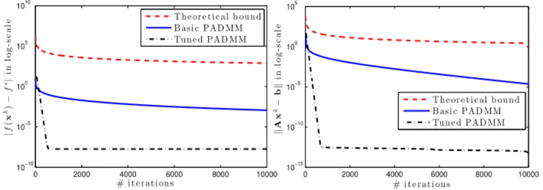
The following corollary shows the convergence of the PADMM scheme (62)-(63), whose proof can be found in [66].