Queen’s Economics Department Working Paper No. 1063
Nested Pseudo-likelihood Estimation and Bootstrap-based
Inference for Structural Discrete Markov Decision Models
Hiroyuki Kasahara
University of Western Ontario
Katsumi Shimotsu
Queen’s University
Department of Economics
Queen’s University
94 University Avenue
Kingston, Ontario, Canada
K7L 3N6
Nested Pseudo-likelihood Estimation and
Bootstrap-based Inference for Structural Discrete
Markov Decision Models
∗Hiroyuki Kasahara Department of Economics University of Western Ontario
[email protected] Katsumi Shimotsu Department of Economics Queen’s University [email protected] February 4, 2006 Abstract
This paper analyzes the higher-order properties of nested pseudo-likelihood (NPL) esti-mators and their practical implementation for parametric discrete Markov decision models in which the probability distribution is defined as a fixed point. We propose a new NPL estima-tor that can achieve quadratic convergence without fully solving the fixed point problem in every iteration. We then extend the NPL estimators to develop one-step NPL bootstrap pro-cedures for discrete Markov decision models and provide some Monte Carlo evidence based on a machine replacement model of Rust (1987). The proposed one-step bootstrap test statistics and confidence intervals improve upon the first order asymptotics even with a rela-tively small number of iterations. Improvements are particularly noticeable when analyzing the dynamic impacts of counterfactual policies.
Keywords: Edgeworth expansion, k-step bootstrap, maximum pseudo-likelihood estima-tors, nested fixed point algorithm, Newton-Raphson method, policy iteration.
JEL Classification Numbers: C12, C13, C14, C15, C44, C63. ∗
We are grateful to Victor Aguirregabiria, Chris Bennett, Christopher Ferrall, Silvia Gon¸calves, Lance Lochner, James MacKinnon, John Rust, and seminar participants at Canadian Econometric Study Group, Indiana Uni-versity, University of Maryland, and Queen’s University for helpful comments. Shimotsu thanks the SSHRC for financial support.
1
Introduction
Understanding the dynamic response of individuals and firms is imperative for properly assess-ing various policy proposals. As numerous empirical studies have demonstrated, the estimation of dynamic structural models enhances our understanding of individual and firm behavior, es-pecially when expectations play a major role in decision making.1
The literature on estimating parametric discrete Markov decision models was pioneered by Rust (1987, 1988) who introduced thenested fixed point algorithm (NFXP). The NFXP requires repeatedly solving the fixed point problem during optimization and can be very costly when the dimensionality of state space is large. Hotz and Miller (1993) developed a simpler estima-tor, called the conditional choice probabilities (CCP) estimator, based on the policy iteration
mapping—denoted by Ψ(P, θ)—which maps an arbitrary choice probability P and the model parameterθto another choice probability. The true choice probability is characterized as a fixed point of the mapping, i.e., Pθ = Ψ(Pθ, θ). The CCP estimates the parameter θ by minimizing
the discrepancy between the observed choice probabilities and Ψ( ˆP0, θ),where ˆP0 is an initial estimate. The CCP requires only one policy iteration to evaluate the objective function, leading to a significant computational gain over the NFXP.
Aguirregabiria and Mira (2002) [henceforth, AM] extended the CCP estimator and proposed thenested pseudo-likelihood (NPL) estimator. Upon obtaining ˆθfrom the CCP, one can update the conditional choice probabilities estimate as ˆP1 = Ψ( ˆP0,θˆ),which provides a more accurate estimator ofPθ than ˆP0. Next, one can obtain another estimator ofθ,θˆ1,by using Ψ( ˆP1, θ)
in-stead of Ψ( ˆP0, θ).Iterating this procedure generates a sequence of the NPL estimators, including the CCP as the initial element and the NFXP estimator as its limit. Somewhat surprisingly, AM showed that the NPL estimator for any number of iterations has the same limiting distribution as the NFXP estimator.
The NPL provides a menu of first-order equivalent estimators that empirical researchers can choose from, but little is known about their higher-order properties. Since the choice among these estimators involves a trade-off between efficiency and computational burden, understanding their higher-order properties is necessary for making an appropriate choice for a given situation.
1
Contributions include Miller (1984), Pakes (1986), Berkovec and Stern (1991), Rust (1987), Keane and Wolpin (1997), Rust and Phelan (1997), Gilleskie (1998), Eckstein and Wolpin (1999), Imai and Keane (2004).
In fact, the simulations by AM reveal that iterating the policy iteration mapping improves the accuracy of the parameter estimates, often by a substantial magnitude, suggesting that higher-order properties may be of practical importance.
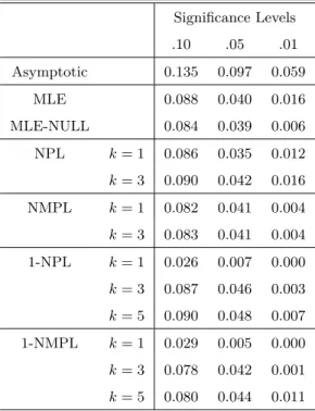
We present the simulation results showing that tests based on first order asymptotics can be unreliable. While bootstrap tests are known to provide a better inferential tool than first-order asymptotic approximations, few studies have analyzed a bootstrap-based inference method for discrete Markov decision models. The main obstacle lies in the computational burden, because the bootstrap requires repeated parameter estimation under different simulated samples while it is not unusual for estimating one set of the parameters to take more than a day. This further increases the need for computationally attractive methods. Moreover, because the asymptotic improvement of the bootstrap relies on its higher-order properties, analyzing those properties is essential for practical applications.
The contributions of this paper are three-fold. First, we analyze the higher-order properties of the NPL estimator and derive the stochastic differences [c.f., Robinson (1988)] between the NFXP and the sequence of estimators generated by the NPL algorithm. We show the rate at which the sequence of the NPL estimators approaches the NFXP and provide a theoretical explanation for the simulation results in AM, in which iterating the NPL algorithm improves the accuracy of the NPL estimator.
Second, we propose two new estimators based on the NPL estimator. First, we develop a
nested modified pseudo-likelihood (NMPL) estimator that uses a pseudo-likelihood defined in terms of two policy iterations as opposed to one policy iteration in the NPL. We show the convergence rate of the NMPL is faster than quadratic while that of the NPL is less than quadratic. Second, we propose a version of the NPL and NMPL estimators, called the one-step NPL and NMPL estimators, that use only one Newton-Raphson (NR) step to update the parameterθduring each iteration. By using only one NR step rather than fully solving the pseudo-likelihood problem for every iteration, we can reduce the computational cost significantly. The one-step NMPL estimator with the NR method achieves a quadratic convergence while the convergence rate of the one-step NPL estimator is less than quadratic.
Our one-step NPL and NMPL estimators are closely related to the k-step estimators ana-lyzed by Pfanzagl (1974), Janssen, Jureckova, and Veraverbeke (1985), Robinson (1988), and Andrews (2002a), among others. Specifically, our one-step estimators may be viewed as a
(semi-parametric)k-step estimator in which an estimate of nuisance parameterP is updated between NR steps.
The key to understanding the convergence properties of the NPL and the NMPL algorithms is the orthogonality condition between the parameter of interestθ and the nuisance parameter
P. When we define a pseudo-likelihood in terms of two policy iterations, θ and P become
orthogonal in any sample size. This strengthens one of the key properties of the NPL that θ
and P areasymptotically orthogonal. Consequently, the effect of the nuisance parameter P on the estimation of θ becomes negligible at a faster rate in the NMPL than in the NPL, leading to their different convergence rates.
The superior convergence properties of the NMPL over the NPL is not without cost. The computational cost for each NR step is larger in the NMPL, because its pseudo-likelihood is defined in terms of two policy iterations in contrast to one policy iteration in the NPL. Comparing the number of policy iterations required to achieve a particular level of convergence suggests that the overall computational cost of the one-step NMPL may be lower than that of the one-step NPL when the target level of convergence is high.
Third, we develop a computationally attractive bootstrap procedure for parametric dis-crete Markov decision models, applying the framework developed by Davidson and MacKinnon (1999a) and Andrews (2002b, 2005). Starting with an estimate from the original sample, a boot-strap estimator is obtained with the bootboot-strap sample by using the (one-step) NPL and NMPL, where taking a small number of iterations suffices to achieve higher-order improvements. Since their computational burden is substantially less than that of the NFXP, our proposed bootstrap is feasible for many discrete Markov decision models where the standard bootstrap procedure is too costly to implement. The computational burden is further reduced because the covari-ance matrix can be consistently estimated in the bootstrap sample using the derivatives of a
pseudo-likelihood function instead of the likelihood function based on the fixed point solution. The proofs of higher-order properties of the proposed algorithm build on the results developed in Andrews (2002a,b, 2005).
We also consider two extensions of our bootstrap procedure: counterfactual experiments and models with unobserved heterogeneity. When estimated structural models are used to quantitatively assess the impact of counterfactual policies, the reliability of the estimated impact arises as an important issue. We develop a bootstrap procedure that allows us to construct
reliable CIs for the impact of counterfactual policies where asymptotic CIs may be unreliable. We also show that our bootstrap procedure can be applied to a finite mixture model, which is a popular approach when preferences are likely to be different across individuals.
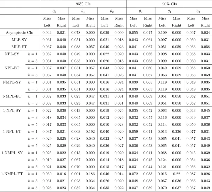
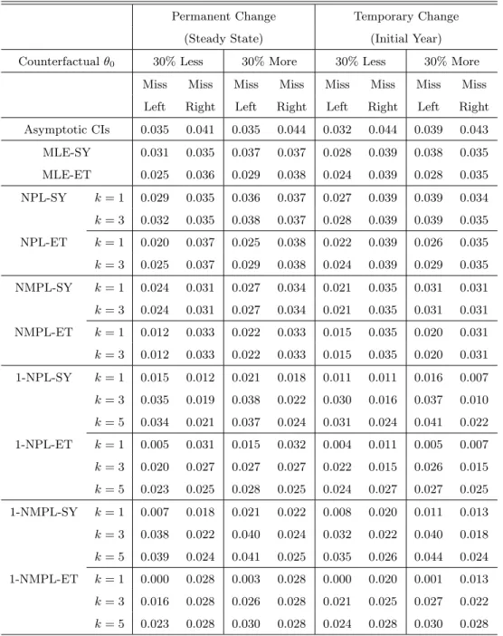
In order to assess the performance of our bootstrap procedure, we provide Monte Carlo evidence based on a machine replacement model of Rust (1987) and Cooper, Haltiwanger, and Power (1999). We compare the performance of the bootstrap CIs for the impact of counter-factual policies with that of the asymptotic CIs. The bootstrap CIs perform better than the asymptotic CIs, and the one-step bootstrap CIs with a few iterations often achieve a similar performance to the bootstrap CIs based on the NFXP. The simulation results suggest that we may construct more reliable CIs by using our proposed one-step bootstrap procedure without facing a prohibitive computational burden.
The remainder of the paper is organized as follows. Section 2 introduces the model. In Section 3, we propose and analyze a modification to the NPL estimator. Section 4 describes our one-step estimation algorithm and proves its convergence properties. Section 5 analyzes the higher-order improvements from applying parametric bootstrapping to the one-step NPL estimators. Practical extensions are discussed in Section 6, and Section 7 reports some simulation results. Proofs and technical results are collected in Appendices A and B.
2
The Econometric Model
This section introduces the class of discrete Markov decision models considered in this paper. We closely follow the setup and the notations of Aguirregabiria and Mira (2002) [AM, hereafter]. An agent maximizes the expected discounted sum of utilities, E[P∞
j=0βjU(st+j, at+j)|at, st],
wherestis the vector of states and at is an action to be chosen from the discrete and finite set
A={1,2, ..., J}. The transition probabilities are given by p(st+1|st, at). The Bellman equation
for this dynamic optimization problem is written as
W(st) = max a∈A U(st, a) +β Z W(st+1)p(dst+1|st, a) .
¿From the viewpoint of an econometrician, the state vector can be partitioned asst = (xt, t),
wherext is observable andtis unobservable. We consider the following assumptions.
separable in the utility function so that U(st, at) = u(xt, at) +t(at), where t(at) is the
a-th element of the unobservable state vector t={t(a) :a∈A}.
Assumption 2 (Conditional Independence): The transition probability of the state vari-ables can be written as p(st+1|st, at) =g(t+1|xt+1)f(xt+1|xt, at), where g(|x) has finite
first moments and is twice differentiable in uniformly in x ∈ X; the support of (a) is the real line for alla.
Assumption 3: The observable state variable xt has compact supportX⊂Rd.
Assumptions 1 and 2 are analogous to Assumptions 1 and 2 in AM. They are first introduced by Rust (1987) and widely used in the literature. Assumption 3 admitsxtto have a continuous
distribution, relaxing Assumption 3 in AM that assumesxthas a finite support.
Define the integrated value function V(x) = R W(x, )g(d|x), and let BV be the space of
V ≡ {V(x) :x ∈X}.The Bellman equation can be rewritten in terms of this integrated value function as: V(x) = Z max a∈A u(x, a) +(a) +β Z X V(x0)f(dx0|x, a) g(d|x). (1)
Let Γ(·) be the Bellman operator defined by the right-hand side of the above Bellman equation. The Bellman equation is compactly written asV = Γ(V).
Let P(a|x) denote the conditional choice probabilities of the action agiven the observable state x, and let BP be the space of {P(a|x) : x ∈ X}. Given the value function V, P(a|x) is
expressed as P(a|x) = Z I a= arg max j∈A[v(x, j) +(j)] g(d|x), (2)
where v(x, a) = u(x, a) +βRXV(x0)f(dx0|x, a) is the choice-specific value function and I(·) is an indicator function. The right-hand side of the equation (2) can be viewed as a mapping from one Banach (B-) spaceBV to another B-space BP. Define the mapping Λ(V) :BV →BP as
[Λ(V)](a|x)≡ Z I a= arg max j∈A[v(x, j) +(j)] g(d|x). (3)
We now derive the mapping from choice probabilities to value functions based on Hotz and Miller (1993). First, the Bellman equation (1) can be rewritten as
V(x) =X a∈A P(a|x) u(x, a) +E[(a)|x, a; ˜vx, P(a|x)] +β Z X V(x0)f(dx0|x, a) (4)
where
E[(a)|x, a; ˜vx, P(a|x)] = [P(a|x)]−1
Z
(a)I{v˜(x, a) +(a)≥v˜(x, j) +(j), j ∈A}g(d|x),
where ˜v(x, a) =v(x, a)−v(x,1) and ˜vx ≡ {v˜(x, a) :a >1}.
DefinePx ≡ {P(a|x) :a >1}. For eachx, there exists a mapping from the utility differences
˜
vx to the conditional choice probabilities Px. Denote this mapping as Px = Qx(˜vx). Hotz
and Miller (1993) showed that this mapping is invertible so that the utility differences can be expressed in terms of the conditional choice probabilities: ˜vx = Q−x1(Px). Invertibility allows
us to express the conditional expectations of (a) in terms of the choice probabilities Px as
ex(a, Px)≡E[(a)|x, a;Q−x1(Px), P(a|x)].
By substituting these functions into (4), we obtain
V(x) =uP(x) +βEPV(x), (5) whereuP(x) = P a∈AP(a|x)[u(x, a)+ex(a, Px)] andEPV(x) = P a∈AP(a|x) R XV(x 0)f(dx0|x, a).
Here,uP is the expected utility function implied by the conditional choice probabilityPxwhereas
EP is the conditional expectation operator for the stochastic process{xt, at}induced by the
con-ditional choice probabilityP(at|xt) and the transition densityf(xt+1|xt, at).
Define P ≡ {Px :x∈X}. The value function implied by the conditional choice probability
P is a unique solution to the linear operator equation (5): V = (I−βEP)−1uP. The right-hand
side of this equation can be viewed as a mapping from the choice probability space BP to the
value function spaceBV. Define this mapping as ϕ(P)≡(I −βEP)−1uP. Then we may define
a policy iteration operator Ψ as a composite operator ofϕ(·) and Λ(·):
P = Ψ(P)≡Λ(ϕ(P)).
Given the fixed point of this policy iteration operator,P, the fixed point of the Bellman equation (1) can be expressed asV =ϕ(P).
Before proceeding, we collect some definitions. Because P and V are infinite dimensional whenxtis continuously distributed, the derivatives of Ψ,Λ,andϕneed to be defined as Fr´echet
(F-) derivatives. For a mapg:X →Y, whereX and Y are B-spaces, g is F-differentiable atx
iff there exists a linear and continuous mapT such that
for all h in some neighborhood of zero, where || · || is an appropriate norm (e.g. sup norm, Euclidean norm if g ∈RM). If it exists, this T is called the F-derivative of g at x, and we let
Dg(x) denote the F-derivative of g. Note that Dg(x) is an operator. When X is a Euclidean space, the F-derivative coincides with the standard derivative dg(x)/dx. Concepts such as the chain rule, product rule, higher-order and partial derivatives, and Taylor expansion are defined analogously to the corresponding concepts defined for the functions in Euclidean spaces. For further details the reader is referred to Zeider (1986). Ichimura and Lee (2004) provide a concise summary on F-derivatives. Let Djg(x, y) denote the jth order F-derivative of g(x, y), and let
Dxg(x, y) denote the partial F-derivative ofg(x, y) with respect tox.Ifxis a finite dimensional
parameter,Dxg(x, y) is equal to the standard partial derivative ∂g(x, y)/∂x.
One of the important properties of the policy iteration operator Ψ is that the derivative of Ψ inP is zero at the fixed point. AM proves this property in the case where the support ofxt
is finite. The following proposition establishes that this zero-Jacobian property also holds even when the support ofxt is not finite andV does not belong to a Euclidean space.
Proposition 1 Suppose Assumptions 1 - 3 hold. Thenϕ(·)is F-differentiable at the fixed point
P. If Ψ(·) is F-differentiable at P, then Dϕ(·) =DΨ(·) = 0 (zero operator) if evaluated at the fixed point P. In other words,Dϕ(P)ξ =DΨ(P)ξ = 0 for any ξ∈BP.
3
Maximum Likelihood Estimator and its Variants
We consider a parametric model by assuming that the utility function and the transition prob-abilities are unknown up to an Lθ×1 parameter vector θ ≡ (θu, θg, θf), where θu, θg, and θf
are the parameter vectors in the utility function u, the density of unobservable state variables
g, and the conditional transition probability function f, respectively. Consequently, the policy iteration operator Ψ is parameterized as Ψ(P, θ) = Λ(ϕ(P, θ), θ). This corresponds to AM’s notation Ψθ(P).
Let Pθ denote the fixed point of the policy iteration operator so that Pθ = Ψ(Pθ, θ). Let
{wi : i = 1,2, ..., N} be a random sample of w = (a, x0, x) from the population, where xi
is drawn from the stationary distribution implied byPθ and fθf,ai is drawn conditional on xi
can be decomposed into conditional choice probability and transition probability terms as: lN(θ) =lN,1(θ) +lN,2(θf) = N X i=1 lnPθ(ai|xi) + N X i=1 lnfθf(x0i|xi, ai). (6)
Since θf can be estimated consistently without having to solve the Markov decision model, we
focus on the estimation ofα≡(θu, θg) given initial consistent estimates ofθf from the likelihood
lN,2(θf).Thus, Ψ(P, θ) = Ψ(P, α, θf),and we use both Ψ(P, θ) and Ψ(P, α, θf) henceforth.
The maximum likelihood estimator solves the following constrained maximization problem:
max α 1 N N X i=1 lnP(ai|xi) s.t. P = Ψ(P, α,θˆf). (7)
Rust (1987) develops the celebrated Nested Fixed Point (NFXP) algorithm by formulating the parameter restriction in terms of Bellman’s equation. The NFXP repeatedly solves the fixed point problem at each parameter value to maximize the likelihood with respect toα. Let ˆαdenote the solution to the maximization problem (7), and let ˆP denote the associated conditional choice probability estimate characterized by the fixed point: ˆP = Ψ( ˆP ,α,ˆ θˆf).
3.1 Nested Pseudo-likelihood (NPL) Estimator
Assuming an initial consistent estimator ˆP0 is available, the nested pseudo-likelihood (NPL) estimator developed by AM is recursively defined as follows.
Step 1: Given ˆPjP L−1,updateα by
ˆ αP Lj = arg max α 1 N N X i=1 ln Ψ(α,PˆjP L−1,θˆf)(ai|xi).
Step 2: UpdateP using the obtained estimate ˆαP Lj by ˆPjP L = Ψ( ˆPjP L−1,αˆP Lj ,θˆf).
Iterate Steps 1-2 until j=k.
LetP0 be the true set of conditional choice probabilities, and let f0 be the true conditional transition probability ofx. Let Θα and Θf be the set of possible values ofα and θf,and define
Θ = Θα×Θf.Following AM, consider the following regularity conditions:
Assumption 4. (a) Θα and Θf are compact. (b) Ψ(P, α, θf) is three times continuously
BP ×Θα×Θf.(d)wi={ai, x0i, xi},fori= 1,2, . . . , N,are independently and identically
distributed, anddF(x)>0 for any x in the support of xi, where F(x) is the distribution
function ofxi. (e) There is a uniqueθ0f ∈int(Θf) such that, for any (a, x, x0)∈A×X×X,
fθ0
f(x
0|x, a) =f0(x0|x, a). (f) There is a uniqueα0 ∈int(Θ
α) such that, for any (a, x)∈A×
X, Pθ0(a|x) =P0(a|x). For anyα 6=α0,Prθ0({(a, x) : Ψ(P0, α, θ0f)(a|x)6=P0(a|x)}) >0.
(g)Eθ0sup(P,α,θf)||DsΨ(P, α, θf)(a|x)||2 <∞ fors= 1, . . . ,4. (h) ˆθf −θf0 =Op(N−1/2),
ˆ
P0P L−P0 =op(1),and the NFXP estimator ˆα satisfies
√
N( ˆα−α0)→dN(0,Ω).
Assumptions 4(a)–4(f) are similar to the regularity conditions 4(a)-(f) in AM. The supremum in 4(g) may be taken in a neighborhood of (P0, α0, θ0f).
Following Robinson (1988), for matrix/mapping and (nonnegative) scalar sequences of ran-dom variables {XN, N ≥1} and {YN, N ≥1},respectively, we write XN =Op(YN)(op(YN)) if
||XN|| ≤CYN for some (all)C >0 with probability arbitrarily close to one for sufficiently large
N.
Our first main result shows that the NPL estimator converges to the MLE, ˆα,at a superlinear, but less than quadratic, convergence rate.
Proposition 2 Suppose Assumptions 1-4 hold. Then, for k= 1,2, . . .
ˆ
αP Lk −αˆ=Op(N−1/2||PˆkP L−1−P||ˆ +||PˆkP L−1−Pˆ||2), PˆkP L−Pˆ =Op(||αˆP Lk −α||ˆ ).
This proposition provides a theoretical explanation for the result of the AM’s Monte Carlo experiment. Their experiment illustrates that the finite sample properties of the NPL estimators improve monotonically withkand that the estimators withk= 2 or 3 substantially outperform the estimator withk= 1.
Note that ˆP0P L −P0 = Op(N−b) with b > 1/4 suffices for
√
N( ˆαP Lk −α0) →d N(0,Ω) for all k ≥ 1. This weakens assumption (g) of Proposition 4 of AM and also implies that the NPL estimator is valid even if xt has an infinite support and a kernel-based estimator is used
to estimate P0. The result suggests that the NPL algorithm may work even with relatively imprecise initial estimates of the conditional choice probabilities.
If ˆP0P L−P0 =Op(N−b) withb∈(1/4,1/2],repeated substitution gives
ˆ
In particular, if the support of xt is finite and we can obtain ˆP0P L such that ˆP0P L −P0 =
Op(N−1/2),then the convergence rate becomesN−(k+1)/2.
3.2 Nested Modified Pseudo-likelihood (NMPL) Estimator
We now introduce the nested modified pseudo-likelihood (NMPL) estimator that achieves a faster rate of convergence than the NPL estimator:
Step 1: Given ˆPjM P L−1 ,updateα by
ˆ αM P Lj = arg max α 1 N N X i=1 ln Ψ2( ˆPjM P L−1 , α,θˆf)(ai|xi), where Ψ2(P, α, θf)(ai|xi)≡Ψ(Ψ(P, α, θf), α, θf)(ai|xi).
Step 2: UpdateP using the obtained estimate ˆαM P Lj by ˆPjM P L= Ψ( ˆPjM P L−1 ,αˆM P Lj ,θˆf).
Iterate Steps 1-2 until j=k.
Assumption 5. (a) For any α 6= α0, Prθ0({(a, x) : Ψ2(P0, α, θ0f)(a|x) 6= P0(a|x)}) > 0. (b)
Eθ0sup(P,α,θ
f)||D sΨ
2(P, α, θf)(ai|xi)||2 <∞ fors= 1, . . . ,4. (c) ˆP0M P L−P0 =op(1).
The following proposition shows the NMPL estimator of α converges at a rate faster than quadratic while the NMPL estimator ofP converges at a quadratic rate.
Proposition 3 Suppose Assumptions 1-5 hold. Then, for k= 1,2, . . .
ˆ
αM P Lk −αˆ=Op(N−1/2||PˆkM P L−1 −Pˆ||2+||PˆkM P L−1 −Pˆ||3), PˆkM P L−Pˆ =Op(||PˆkM P L−1 −Pˆ||2).
If ˆP0M P L−P0=Op(N−b) withb∈(0,1/2],then the convergence rate is given by
ˆ αM P Lk −αˆ =Op(N−1/2−b2 k +N−3b2k−1), PˆkM P L−Pˆ =Op(N−b2 k ).
In particular, if ˆP0M P L−P0 = Op(N−1/2), then we have ˆαM P Lk −αˆ =Op(N−1/2−2 k−1
). Note that ˆPM P L
0 −P0 =Op(N−b) withb >1/6 suffices for
√
N( ˆαM P L
k −α0)→dN(0,Ω) for allk≥1.
Therefore, the NMPL estimator requires a weaker condition on the initial estimate of P0 than the NPL estimator. The NMPL estimator may, therefore, be preferable to the NPL estimator
when we only have a poor initial estimate of P0, as is likely to be the case, for instance, in models with unobserved heterogeneity.
Using Ψ2(P, α, θf) instead of Ψ(P, α, θf) achieves a faster rate of convergence. However, the
NMPL algorithm requires more policy iterations than the NPL for computing each ˆαj, which
implies that the overall computational cost for achieving a given rate of convergence may be higher with the NMPL.
The following two orthogonality conditions between ˆα and ˆP are the key to understanding the difference in the rates of convergence between the NPL and the NMPL estimators:2
N−1PN i=1DP αln Ψ(Pθˆ,θˆ)(ai|xi) =Op(N −1/2), N−1PN i=1DP αln Ψ2(Pθˆ,θˆ)(ai|xi) = 0. (9)
Thus, at the fixed point, ˆα and ˆP areasymptotically orthogonal in the NPL while they are orthogonal in any sample size in the NMPL. In case of the NPL, the asymptotic orthogonality in the first equation of (9) implies that the estimation error ˆPkP L−1−Pˆ has an asymptotically negligible effect on ˆαP Lk −α,ˆ diminishing at the rate of N−1/2. Since the extent to which the impreciseness of ˆPkP L−1 would be carried over to the estimate ˆαP Lk is mitigated only at the rate of N−1/2, the NPL converges at a superlinear, but less than quadratic, rate. In case of the NMPL, the second equation of (9) implies that ˆPkM P L−1 −Pˆ has, at most, a second-order effect on ˆαM P Lk −αˆ for any sample size N and hence the NMPL converges, at least, at a quadratic rate. In the appendix, we also show thatN−1PN
i=1DP P αln Ψ2(Pθˆ,θˆ)(ai|xi) =Op(N
−1/2) [c.f., Lemma 9(b)], implying that the second-order effect is diminishing at the rate of N−1/2, and thus the NMPL converges at a faster rate than quadratic.
3.3 Covariance Matrix Estimation and Test Statistics
Suppose ˆθf is obtained by maximizing lN,2(θf). Suppress (a|x) and (x0|x, a) from Pθ(a|x) and
fθf(x0|x, a). Expanding the first order condition for ˆα and ˆθf gives the asymptotic covariance
matrix of ˆθ= ( ˆα0,θˆf0)0 as
Σ(θ0) =D(θ0)−1V(θ0)(D(θ0)−1)0,
where D(θ) = D11(θ) D12(θ) 0 D22(θ) =− E(∂2/∂α∂α0) lnPθ E(∂2/∂α∂θ0f) lnPθ 0 E(∂2/∂θf∂θf0) lnfθf , V(θ) = V11(θ) V12(θ) V21(θ) V22(θ) =E (∂/∂α) lnPθ (∂/∂θf) lnfθf (∂/∂α) lnPθ (∂/∂θf) lnfθf 0 .
The information matrix equality from the MLE based onlN,2(θ) alone impliesD22(θ0) =V22(θ0),
and the information matrix equality from the full MLE based onlN(θ) impliesD11(θ0) =V11(θ0) and−E(∂2/∂α∂θ0f) lnPθ0 =E(∂/∂α) lnPθ0(∂/∂θ0f)(lnPθ0 + lnfθ0
f).
There are several ways to estimate Σ(θ0) consistently. Let DN(θ) and VN(θ) be the sample
analogue ofD(θ) and V(θ), respectively, and define
DON(θ) = 1 N N X i=1 (∂/∂α) lnPθ(∂/∂α0) lnPθ (∂/∂α) lnPθ(∂/∂θ0f)(lnPθ+ lnfθf) 0 (∂/∂θf) lnfθf(∂/∂θf0) lnfθf .
DNO(θ) is an outer-product-of-the-gradient (OPG) estimator ofD(θ),which does not require the calculation of the second derivatives of lnPθ and lnfθf.Then one can use ΣN = ΣN(¯θ),where
¯
θis a consistent estimate of θ0 and
ΣN(θ) = DN(θ)−1VN(θ)(DN(θ)−1)0, or (10) ΣN(θ) = DON(θ) −1V N(θ)(DNO(θ) −1)0 .
The consistency of ΣN(¯θ) follows from the standard argument. Notice, however, that computing
ΣN(¯θ) potentially requires a large number of policy iterations, being based on the full solution
of the fixed point problem.
Alternatively, we may estimateV(θ) andD(θ) using the pseudo-likelihood function defining the NPL and NMPL estimators. DefineDNP L(P, θ) andDNM P L(P, θ) by replacingPθ in the
defi-nition ofDN(θ) with Ψ(P, θ) and Ψ2(P, θ),respectively, and define DNO,P L(P, θ), DO,M P LN (P, θ),
VNP L(P, θ), and VNM P L(P, θ) analogously. As shown in the following Proposition, we can esti-mate Σ(θ0) consistently using these estimates with the NPL and NMPL estimators of (P, α) and constructt- and Wald statistics with a limited number of policy iterations.
Proposition 4 Let P¯ and θ¯denote estimators that converge to P0andθ0 in probability. Then,
Let θr, θr0,and ˆθr denote the r-th elements of θ, θ0,and ˆθ respectively. Let (ΣN)rr denote
the (r, r)-th element of ΣN.The t-statistic for testing the null hypothesis H0 :θr=θr0 is
TN(θ0r) =N1/2(ˆθr−θ0r)/(ΣN)1rr/2.
Letη(θ) be anRLη-valued function that is continuously differentiable at θ0. The Wald statistic
for testingH0 :η(θ0) = 0 versusHA:η(θ0)6= 0 is
WN(θ0) = HN(ˆθ, θ0)0HN(ˆθ, θ0), where HN(θ, θ0) = ∂ ∂θ0η(θ)ΣN(θ) ∂ ∂θη(θ) −1/2 N1/2η(θ).
ThenTN(θr0)→dN(0,1) and WN(θ0)→dχ2Lη under the null hypotheses.
4
One-step NPL and NMPL Estimators
We propose one-step NPL and NMPL estimators which update the parameter α using one Newton step without fully solving the optimization problem. This reduces the computational cost of the corresponding estimators especially when the dimension ofαis high. LetLN(P, α, θf)
denote the objective function of the NPL estimator as
LN(P, α, θf) = 1 N N X i=1 ln Ψ(P, α, θf)(ai|xi). (11)
The one-step NPL estimator, ( ˜αP Lk ,P˜kP L),is defined recursively as:
Step 1: Given ( ˜PjP L−1,α˜P Lj−1,θˆf), update α by
˜ αP Lj = ˜αP Lj−1−(QN,j−1)−1 ∂ ∂α0LN( ˜P P L j−1,α˜P Lj−1,θˆf), (12) whereQN,j−1=QN( ˜PjP L−1,α˜P Lj−1,θˆf).
Step 2: UpdateP using the policy iteration operator evaluated at the updated ˜αP Lj :
˜
PjP L = Ψ( ˜PjP L−1,α˜P Lj ,θˆf).
The matrixQN,j−1determines whether the one-step NPL estimator uses the NR, default NR, line-search NR, or Gauss-Newton (GN) steps. The NR choice ofQN,j−1 isQN,jN R−1 = (∂2/∂α∂α0)
LN( ˜PjP L−1,α˜P Lj−1,θˆf). The default NR choice of QN,j−1, denoted QDN,j−1 equals QN RN,j−1 if ˜αP Lj
defined in (12) satisfiesLN( ˜PjP L−1,α˜P Lj ,θˆf) ≥LN( ˜PjP L−1,α˜jP L−1,θˆf),but equals some other matrix
otherwise. Typically, (1/ε)Idim(α) for some small ε > 0 is used. The line-search NR choice,
QLSN,j−1, computes ˜αP L,λj for λ∈ (0,1] using (1/λ)QN RN,j−1 and chooses the one that maximizes the objective function. The GN choice, denotedQGNN,j−1, uses a matrix that approximates the NR matrixQN RN,j−1.A popular choice is the OPG estimator
QOP GN,j−1=− 1 N N X i=1 ∂ ∂αln Ψ( ˜P P L j−1,α˜P Lj−1,θˆf)(ai|xi) ∂ ∂α0 ln Ψ( ˜P P L j−1,α˜P Lj−1,θˆf)(ai|xi),
because this does not require the calculation of the second derivative of the objective function. The following proposition establishes that the one-step NPL estimator achieves a similar rate of convergence to the original NPL estimator. This is because taking one NR step brings the one-step NPL estimator sufficiently close to the NPL estimator. In fact, the distance between the one-step NPL estimator and the NPL estimator is at most of the same order of magnitude as the distance between the NFXP estimator and the NPL estimator.
Proposition 5 Suppose the assumptions of Proposition 2 hold and the initial estimates( ˜αP L0 ,P˜0P L)
are consistent. Then, fork= 1,2, . . . ,
˜ αkP L−αˆ = Op(||α˜P Lk−1−α||ˆ 2+N −1/2||P˜P L k−1−Pˆ||+||P˜kP L−1−P||ˆ 2) [+Op(N−1/2||αˆ−α˜P Lk−1||) for OPG ], ˜ PkP L−Pˆ = Op(||α˜P Lk −α||ˆ ).
If the initial estimates satisfy ˜αP L0 −α0,P˜0P L −P0 = Op(N−b) with b ∈ (1/4,1/2], then
repeated substitution gives3
˜
αP Lk −αˆ =Op(N−(k−1)/2−2b), P˜kP L−Pˆ=Op(N−(k−1)/2−2b), (13)
3
The initial root-N consistent estimate, ˜αP L0 , can be obtained from applying the original NPL estimator with
k= 1 or using Hotz and Miller’s CCP estimator. Furthermore, when we apply the one-step NPL estimator to the bootstrap-based inference, we may use the estimate from the original sample as an initial root-N consistent estimate for the bootstrap sample.
and the one-step NPL estimator achieves the same convergence rate as the NPL estimator. The one-step NMPL estimator ( ˜αM P Lk ,P˜kM P L) is defined analogously usingN−1PN
i=1ln Ψ2(P, α, θ)(ai|xi)
asLN(P, α, θ).As shown in the following proposition, it achieves the quadratic rate of
conver-gence when the NR, default NR, or line-search NR is used. When the OPG is used, however, its convergence rate reduces to that of the one-step NPL estimator.
Proposition 6 Suppose the assumptions of Proposition 3 hold and the initial estimates( ˜αM P L0 ,P˜0M P L)
are consistent. Then, fork= 1,2, . . . ,
˜ αkM P L−αˆ = Op(||α˜M P Lk−1 −α||ˆ 2+N −1/2||P˜M P L k−1 −Pˆ||2+||P˜kM P L−1 −Pˆ||3) [+Op(N−1/2||α˜M P Lk−1 −α||ˆ +||P˜kM P L−1 −Pˆ||2) for OPG ], ˜ PkM P L−Pˆ = Op(||α˜M P Lk −α||ˆ +||P˜kM P L−1 −Pˆ||2).
When the initial estimates satisfy ˜αP L0 −α0,P˜0P L −P0 = Op(N−b) with b ∈ (1/4,1/2],
repeated substitution gives
˜
αM P Lk −αˆ = Op(N−b2 k
), P˜kM P L−Pˆ=Op(N−b2 k
), for NR, default NR, line-search NR
˜
αM P Lk −αˆ = Op(N−(k−1)/2−2b), P˜kM P L−Pˆ =Op(N−(k−1)/2−2b), for OPG.
For the NR, the default NR, and the line-search NR, the result follows from a quadratic convergence of NR iterations. For the OPG estimator, the convergence rate is less than quadratic because the matrix QOP GN,j−1 approximates (∂2/∂α∂α0)LN, leading to an approximation error of
the magnitudeOp(N−1/2) in the NR search direction.
Comparing the number of policy iterations required to achieve a particular level of con-vergence with these estimators reveals that the one-step NMPL estimator requires fewer policy iterations than the one-step NPL estimator when the target level of convergence is high. We may also consider a hybrid algorithm that needs the fewest policy iterations by using the one-step NPL estimator for the first few steps and then switching to the one-step NMPL estimator.
5
Parametric Bootstrap and Higher-order Improvements
In this section, building upon Andrews (2005), we analyze the higher-order improvements from applying parametric bootstrapping to the parametric discrete Markov decision models.
5.1 The NFXP Parametric Bootstrap
First, consider bootstrapping the NFXP estimator. The parametric bootstrap sample {wi∗ :
i= 1, . . . , n} is generated using the parametric density at the (unrestricted) NFXP estimator ˆα
and the MLE ˆθf.The conditional distribution of the bootstrap sample given ˆθ= ( ˆα0,θˆ0f) 0 is the
same as the distribution of the original sample except that the true parameter is ˆθ rather than
θ0= (α00, θf00)0.4
The bootstrap estimator θ∗ = (α∗0, θ∗0f)0 is defined exactly as the original estimator ˆθ but using the bootstrap sample{w∗i :i= 1, . . . , n}.Specifically,
θ∗f = arg max θf∈Θf l∗N,2(θf), where l∗N,2(θf) = 1 N N X i=1 lnfθf(x 0∗ i |x ∗ i, a ∗ i), (14) α∗ = arg max α∈Θα 1 N N X i=1 lnP(a∗i|xi∗) s.t. P = Ψ(P, α, θf∗).
The bootstrap covariance matrix estimator, Σ∗N, is defined as Σ∗N(θ∗) where Σ∗N(θ) has the same definition as ΣN(θ) in (10) but with the bootstrap sample in place of the original sample.
The bootstraptand Wald statistics are defined as
TN∗(ˆθr) = N1/2(θ∗r−θˆr)/(Σ∗N)1rr/2, (15) WN∗(ˆθ) = HN∗(θ∗,θˆ)0HN∗(θ∗,θˆ), where HN∗(θ,θˆ) = ∂ ∂θ0η(θ)Σ ∗ N(θ) ∂ ∂θη(θ) −1/2 N1/2(η(θ)−η(ˆθ)),
whereθ∗r denotes ther-th element ofθ∗,and (Σ∗N)rr denotes the (r, r)-th element of Σ∗N.Here,
we use the bootstrap Wald statistics to testH0:η(θ0) = 0 versusHA:η(θ0)6= 0.
Letz|∗T|,α, zT,α∗ ,and zW∗ ,αdenote the 1−αquantiles of|T∗
N(ˆθr)|, TN∗(ˆθr),and WN∗(ˆθ),
respec-tively. The symmetric two-sided bootstrap CI forθr0 of confidence level 100(1−α)% is
CISY M(ˆθr) = [ˆθr−z|∗T|,α(ΣN(ˆθ))
1/2
rr /N1/2,θˆr+z|∗T|,α(ΣN(ˆθ))
1/2
rr /N1/2]. (16)
The equal-tailed two-sided bootstrap CI forθr0 of confidence level 100(1−α)% is
CIET(ˆθr) = [ˆθr−zT,α/∗ 2(ΣN(ˆθ))rr1/2/N1/2,θˆr−z∗T,1−α/2(ΣN(ˆθ)) 1/2
rr /N1/2]. (17)
4
If xi is assumed to be exogenous, then x∗i = xi needs to be used. If xi is assumed to be drawn from its
stationary distributionλ(θ) implied byPθ andfθf, thenx
∗
The symmetric two-sided bootstrapttest ofH0:θr=θr0versusH1 :θr6=θ0r at significance level
αrejectsH0 if|TN(θ0r)|> z|∗T|,α.The equal-tailed two-sided bootstrapttest at significance level
α for the same hypotheses rejects H0 if TN(θ0r) < z∗T,1−α/2 orTN(θ 0
r) > zT,α/∗ 2.The bootstrap Wald test rejectsH0 ifWN(θ0)> z∗W,α.
We introduce technical conditions that are used in establishing the higher-order improve-ments. They mainly consist of the conditions on the higher-order differentiability, the existence of the higher-order moments, and the Cram´er condition. They are essentially the same as Assumptions 4.1-4.3 in Andrews (2005). Letcbe a non-negative constant such that 2cis an in-teger. Let g(wi, θ) = ((∂/∂θ0) lnPθ(a|x),(∂/∂θ0f) lnfθf(x
0|x, a))0,and let h(w
i, θ)∈RLh denote
the vector containing the unique components ofg(wi, θ) and g(wi, θ)g(wi, θ)0 and their partial
derivatives with respect toθthrough orderd= max{2c+ 2,3}.Letλmin(A) denote the smallest eigenvalue of the matrixA.Letd(θ, B) denote the distance between the pointθ and the setB.
We assume the true parameter θ0 lies in a subset Θ0 of Θ and establish asymptotic refine-ments that hold uniformly forθ0 ∈Θ0.For some δ >0,let Θ1 ={θ∈Θ :d(θ,Θ0) < δ/2} and Θ2 ={θ∈Θ :d(θ,Θ0)< δ} be slightly larger sets than Θ0.For the reason why these sets need to be considered, see Andrews (2005).
Assumption 6. (a) Θ1 is an open set. (b) Given any ε > 0, there exists η > 0 such that
||θ−θ0||> εimplies thatEθ0lnPθ0(ai|xi)−Eθ0lnPθ(ai|xi)> η andEθ0lnfθf(x0i|xi, ai)−
Eθ0lnfθf(x0i|xi, ai)> η for all θ∈Θ and θ0 ∈Θ1.(c) supθ0∈Θ
1Eθ0supθ∈Θ||g(wi, θ)||
q0 <
∞,supθ0∈Θ
1Eθ0supθ∈Θ{|lnPθ(ai|xi)|
q0 +|lnf
θf(x0i|xi, ai)|q0}<∞ for allθ ∈Θ for q0 = max{2c+ 1,2}.
Assumption 7. (a)g(w, θ) isd= max{2c+ 2,3} times partially differentiable with respect to
θ on Θ2 for all w= (a, x0, x)∈A×X×X. (b) supθ0∈Θ
1Eθ0||h(wi, θ 0)||q1 <∞ for some q1>2c+ 2.(c) infθ0∈Θ 1λmin(V(θ 0))>0,inf θ0∈Θ 1λmin(D(θ 0))>0.(d) There is a function
Ch(wi) such that ||h(wi, θ)−h(wi, θ0)|| ≤Ch(wi)||θ−θ0||for all θ∈Θ2 andθ0 ∈Θ1 such
that||θ−θ0||< δ and sup
θ0∈Θ 1Eθ0C
q1
h (wi)<∞ for someq1 >2c+ 2.
Assumption 8. (a) For all ε > 0, there exists a positive δ such that for all t ∈ RLh with
||t||> ε, |Eθ0exp(it0h(wi, θ0))| ≤ 1−δ for all θ0 ∈ Θ1. (b) Varθ0(h(wi, θ0)) has smallest
The higher-order differentiability of lnPθ(a|x) and lnfθf(x0|x, a) are satisfied if the
den-sity function of the unobserved state variable, , and the utility function, uθ, are sufficiently
smooth. Note that Assumption 4.1(b) of Andrews (2005) is satisfied by the definition of ˆα
and ˆθf. Assumption 4.1(c) of Andrews (2005) is satisfied with ρ(θ, θ0) = Eθ0lnPθ(a|x) and
Eθ0lnfθf(x0|x, a). Assumption 4.1(d) of Andrews (2005) is satisfied by Assumption 6(b).
Be-causewi is iid, Assumption 4.3(a), (b), and (d) of Andrews (2005) are trivially satisfied, and his
Assumption 4.3(c) reduces to the standard Cram´er condition. Assumption 4.3(f) of Andrews (2005) follows from our Assumption 8(b) since wi is iid. Assumption 8(a), however, is not
satisfied when all elements of the observed state variable have a finite support.
The following Lemma establishes the higher-order improvements of the bootstrap NFXP estimator.
Lemma 1 Suppose Assumptions 1-8 hold with c in Assumptions 6 and 7 as specified below. Then, (a) supθ0∈Θ 0|Prθ0(θ 0 r ∈CISY M(ˆθr))−(1−α)|=O(N−2) for c= 2, (b) supθ0∈Θ 0|Prθ0(θ 0 r ∈CIET(ˆθr))−(1−α)|=o(N−1lnN) for c= 1, (c) supθ0∈Θ 0|Prθ0(WN(θ 0)≤z∗ W,α)−(1−α)|=o(N−3/2lnN) for c= 3/2.
The errors in coverage probability of standard delta method CIs areO(N−1) andO(N−1/2) for symmetric CIs and equal-tailed CIs, respectively. The errors in rejection probability of a standard Wald test areO(N−1).Davidson and MacKinnon (1999b) and Kim (2005) analyze an alternative parametric bootstrap procedure that draws the bootstrap sample using the restricted MLE where the null is imposed. The results in Davidson and MacKinnon and Kim indicate that the bootstrap equal-tailed t-test from the restricted parametric bootstrap have smaller errors in rejection probabilities than the unrestricted parametric bootstrap. In this paper, we mainly focus on CIs, but we conjecture that such a refinement from bootstrapping with the restricted MLE is also possible in our context.
5.2 One-step NPL and NMPL Parametric Bootstrap
Bootstrapping the NFXP estimator is computationally costly because one has to estimate the model repeatedly under different bootstrap samples, where each estimation requires the re-peated full solution of the Bellman equation. For this reason, we propose the one-step
boot-strap NPL and NMPL estimators, which are defined as θ∗kP L = (α∗kP L0, θ∗f0)0 and θk∗M P L = (αk∗M P L0, θf∗0)0,whereθ∗f is defined in (14) and (α∗kP L, Pk∗P L, α∗kM P L, Pk∗M P L) are defined exactly as ( ˜αP Lk ,P˜kP L,α˜kM P L,P˜kM P L) but using the bootstrap sample{wi∗:i= 1, . . . , n}.
We estimateθ by the NFXP estimator in the original sample and use the fixed point at the NFXP estimator Pθˆ as the initial estimate ofP for the one-step estimation with the bootstrap samples. Using the NFXP and Pθˆ does not increase the computational burden significantly, since we are required to estimateθand compute Pθˆ only once in the original sample.5
We use the derivatives of the pseudo-likelihood function defining the NPL or NMPL estimator to construct the covariance matrix estimate (c.f., Proposition 4). This is essential for developing computationally attractive bootstrap-based inference in this context. Evaluating the derivatives of the pseudo-likelihood functions involves a limited number of policy iterations and, under the assumption of extreme-value distributed unobserved state variables, the analytical expression for the first derivatives are available. The computational saving from using the pseudo-covariance matrix estimate can be substantial, since we need to compute the covariance matrix estimates as many times as the number of bootstraps.
With (Pk∗P L, θ∗kP L),we use the bootstrap covariance matrix estimator as
Σ∗N(P, θ) =D∗NO,P L(P, θ)−1VN∗P L(P, θ)(DN∗O,P L(P, θ)−1)0, (18)
whereD∗NO,P L(P, θ) andVN∗P L(P, θ) are the same asDO,P LN (P, θ) andVNP L(P, θ) but constructed with the bootstrap sample. Here, care must be exercised; using the bootstrap covariance ma-trix estimator defined asDN∗P L(Pk∗P L, θk∗P L)−1VN∗P L(Pk∗P L, θ∗kP L)(DN∗P L(Pk∗P L, θ∗kP L)−1)0does not
yield the higher-order refinement, because the second derivatives of lnPθ and ln Ψ(P, θ) with
respect toθdo not agree with each other even when evaluated at the fixed point. With (P∗M P L
k , θk∗M P L),we use either
Σ∗N(P, θ) = DN∗M P L(P, θ)−1VN∗M P L(P, θ)(D∗NM P L(P, θ)−1)0, or
Σ∗N(P, θ) = DN∗O,M P L(P, θ)−1VN∗M P L(P, θ)(DN∗O,M P L(P, θ)−1)0, (19)
5Alternatively, we may estimateθ by the NPL or NMPL estimator in the original sample and use ˆPP L k or
ˆ
PkM P L as the initial estimate for the bootstrap estimation. Here, we focus on the case of estimating θ by the
NFXP estimator but the similar argument applies to the case of estimatingθ by the NPL or NMPL estimator in the original sample.
with analogous definitions for D∗NM P L(P, θ), VN∗M P L(P, θ), and D∗NO,M P L(P, θ). It is important to note thatD∗NM P L(P, θ) must be used ifDN(θ) is used in forming ΣN(θ),andD∗NO,M P L(P, θ)
must be used ifDON(θ) is used in forming ΣN(θ).For instance, usingD∗NM P L(P, θ) whenDON(θ) is
used in forming ΣN(θ) introduces an approximation error of magnitudeOp(N−1/2) and, hence,
does not yield the higher-order refinement.
The one-step bootstrapt- and Wald statistics,TN,k∗ (ˆθr) andWN,k∗ (ˆθ), are defined as in (15),
but with (θ∗,Σ∗N) replaced by (θk∗P L,Σ∗N(Pk∗P L, θk∗P L)) or (θk∗M P L,Σ∗N(Pk∗M P L, θ∗kM P L)). The one-step bootstrap CIs, denotedCISY M,k, CIET,k,are defined analogously to (16) and (17) but
using the 1−α quantiles of |TN,k∗ (ˆθr)|and TN,k∗ (ˆθr) instead of |TN∗(ˆθr)|and TN∗(ˆθr).
Define
µN,k = N−2 k−1
ln2k(N) for the one-step NMPL estimator with NR, default NR, and line-search NR,
µN,k = N−(k+1)/2lnk+1(N) for the one-step NPL estimator and the one-step NMPL estimator with OPG.
Lemma 2 establishes the higher-order equivalence of the one-step NPL and NMPL bootstrap estimators and NFXP bootstrap estimator. Lemma 3 shows, under suitable conditions oncand
k, the difference between the bootstrap test statistics constructed using the one-step NPL or NMPL estimator and the NFXP estimator iso(N−c).
Lemma 2 Suppose Assumptions 1-8 hold for some c > 0 with 2c an integer and supθ∈Θ
||(∂/∂θ)Pθ(a|x)||,sup(P,θ)||DΨ(P, θ)(a|x)||,sup(P,θ)||D2Ψ(P, θ)(a|x)||<∞with probability one.
Then, for all ε >0 and s={P L, M P L},
sup θ0∈Θ 0 Prθ0 Pr∗ˆ θ(||θ ∗s k −θ∗||> µN,k)> N−cε = o(N−c), sup θ0∈Θ 0 Prθ0 Pr∗ˆ θ(|T ∗ N,k(ˆθr)−TN∗(ˆθr)|> N1/2µN,k)> N−cε = o(N−c), sup θ0∈Θ 0 Prθ0 Pr∗θˆ(|WN,k∗ (ˆθ)− WN,k∗ (ˆθ)|> N1/2µN,k)> N−cε = o(N−c),
Lemma 3 Suppose the assumptions of Lemma 2 hold and µN,k =o(N−(c+1/2)). Then, for all
ε >0, sup θ0∈Θ 0 Prθ0 supz∈ R|Ξk(z)|> N −cε =o(N−c), for Ξk(z) = Pr∗θˆ(N1/2(θ∗ks−θˆ)≤z)−Pr ∗ ˆ θ(N 1/2(θ∗−θˆ)≤z)withs={P L, M P L},Pr∗ ˆ θ(T ∗ N,k(ˆθr)≤ z)−Pr∗ˆ θ(T ∗ N(ˆθr)≤z),or Pr ∗ ˆ θ(W ∗ N,k(ˆθ)≤z)−Pr ∗ ˆ θ(W ∗ N(ˆθ)≤z).
Admittedly, the additional finiteness assumptions on the derivatives ofP and Ψ are strong. We conjecture they can be weakened to assumptions in terms of their moments, but doing so would require a longer proof. The following Lemma shows that the errors in coverage probability of the one-step NPL and NMPL bootstrap CIs are the same as those of the NFXP bootstrap CIs. Therefore, the one-step bootstrap estimators achieve the same level of higher-order refinement as the NFXP bootstrap estimator.
Lemma 4 Suppose the assumptions of Lemma 2 hold. (a) Ifc= 2 andµN,k =o(N−5/2), then supθ0∈Θ
0|Prθ0(θ
0
r ∈CISY M,k(ˆθr))−(1−α)|=O(N−2).
(b) Ifc= 1andµN,k=o(N−3/2), thensupθ0∈Θ
0|Prθ0(θ
0
r ∈CIET,k(ˆθr))−(1−α)|=o(N−1lnN).
(c) If c = 3/2 and µN,k = o(N−3/2), then supθ0∈Θ
0|Prθ0(WN(θ
0) ≤ z∗
W,α) −(1−α)| =
o(N−3/2lnN).
The condition µN,k =o(N−5/2) requires k ≥ 3 for the one-step NMPL estimator with the
NR, default NR, and line-search NR, and requiresk≥5 for the one-step NPL estimator and the one-step NMPL estimator with the OPG. Constructing a one-step NMPL bootstrap-t statistic requires 8 policy iterations. This is because the one-step bootstrap NMPL estimator withk= 3 requires 6 policy iterations and the pseudo-covariance matrix estimator based on the second equation of (19) requires 2 policy iterations.6 On the other hand, constructing a one-step NPL bootstrap-t statistic requires 6 policy iterations by using the one-step NPL estimator withk= 5 and using (18), and hence fewer computation. The fewest policy iterations withµN,k=o(N−5/2)
are achieved if we use the one-step NPL estimator in the first and second iterations, the one-step NMPL estimator in the third iteration, and using the pseudo-covariance matrix estimator based on (18); this yieldsµN,k =O(N−3ln6(N)) with 5 policy iterations.
The NPL and NMPL estimators yield the same level of higher-order refinement as stated in Lemma 4 except that, reflecting the difference in their convergence rates, the definition ofµN,k
for the NMPL estimator is different from that for the one-step NMPL estimator. Specifically, we haveµN,k =N−2
k−1−1/2
ln2k+1(N) for the NMPL estimator with NR, default NR, and line search NR. We omit the proof because it is very similar to the proof of Lemmas 2-4.
6
We may reduce the number of policy iterations from 8 to 7 by using the pseudo-covariance matrix estimator (18) instead of (19).
6
Practical Extensions
6.1 Bootstrapping Counterfactual Experiments
One important advantage of structural models over reduced-form models is that we can use them to quantitatively assess the dynamic impact of public policy proposals, often called coun-terfactual experiments. Thereby, the reliability of the estimated impact of policies arises as an important issue. Our proposed bootstrap method allows us to construct reliable CIs for the dynamic impact of counterfactual policies where asymptotic CIs may be unreliable.
Counterfactual policies are characterized by a counterfactual parameter which in turn de-pends on the true parameter. Given the true parameterθ, a counterfactual parameter is denoted by ϑ(θ), where ϑ(·) is a (non-random) smooth mapping from Θ to itself. The quantity of in-terest under a counterfactual policy often depends on the true parameter θ, a counterfactual parameter ϑ(θ), as well as the conditional choice probabilities Pθ and Pϑ(θ); see the examples provided in Section 7. We assume that the quantity of interest takes a scalar value and denote it by y(θ) = g(θ, ϑ(θ), Pθ, Pϑ(θ)). Define Y(θ) = ∂y(θ)/∂θ. In practice, Y(θ) is evaluated by taking a numerical derivative ofy(θ).
Denote the NFXP estimator by ˆθ and the covariance matrix estimator by ΣN(ˆθ). The
asymptotic CI for y(ˆθ) of confidence level 100(1−α) is CIASY = [y(ˆθ)−zα/2σˆy/N1/2, y(ˆθ) +
zα/2σˆy/N1/2], where ˆσ2y =Y(ˆθ)0ΣN(ˆθ)Y(ˆθ) andzα denotes the 1−α quantiles of the standard
normal random variable. It is also straightforward to define the bootstrap CIs fory(ˆθ) . Define the bootstrap t-statistic as Ty =N1/2(y(θ∗)−y(ˆθ))/σ∗y, where σy∗2 = Y(θ∗)0Σ∗N(θ
∗)Y(θ∗) and
θ∗ is the bootstrap NFXP estimator. Let zTy,α∗ and z|∗Ty|,α denote the 1−α quantiles of Ty
and |Ty|. The symmetric and equal-tailed two-sided bootstrap CI for y(ˆθ) of confidence level
100(1−α) are defined as CISY M(y(ˆθ)) = [y(ˆθ) −z|∗Ty|,ασˆy/N
1/2, y(ˆθ) + z∗
|Ty|,ασˆy/N
1/2] and
CIET(y(ˆθ)) = [y(ˆθ)−zTy,α/∗ 2ˆσy/N1/2, y(ˆθ)−z∗Ty,1−α/2σˆy/N1/2], respectively.
Define θ∗ks = (α∗ks0,θˆ0f)0, where s ∈ {P L, M P L}. The one-step NPL or NMPL bootstrap CIs, denoted by CISY M,k(y(ˆθ)) and CIET,k(y(ˆθ)), are defined exactly as CISY M(y(ˆθ)) and
CIET(y(ˆθ)) but with (θ∗,Σ∗N(θ∗)) replaced with (θk∗s,Σ∗N(Pk∗s, θ∗ks)), wheres∈ {P L, M P L}and
Σ∗N(P, θ) is defined by (18)-(19).
When y(θ) depends on Pϑ(θ), constructing the one-step bootstrap CIs often requires com-puting the numerical derivatives of Pϑ(θk∗s) with respect to θk∗s. This is potentially expensive
because it requires solving the fixed point problem, P = Ψ(P, ϑ(θ∗ks)), as many times as the number of bootstraps multiplied by the dimension of θ.7 Letθk∗ denote either θ∗kP L orθ∗kM P L. We propose to reduce the computational burden in computingy(θ) by approximating the fixed point Pϑ(θ∗
k) by taking a finite number of policy iterations under ϑ(θ ∗
k) starting from the fixed
point under ˆθ. That is, starting from Pϑ,k∗0 =Pϑ(ˆθ), we repeat policy iterations under ϑ(θk∗) as
Pϑ,k∗j = Ψ(Pϑ,k∗j−1, ϑ(θk∗)) to obtain a sequence {Pϑ,k∗j :j ≥ 0}. Since Pϑ,k∗0 −Pϑ(θ∗
k) = Op(N −1/2) and the policy iteration mapping Ψ(·, ϑ(θk∗)) has the quadratic convergence property, we have
Pϑ,k∗j −Pϑ(θ∗
k) =Op(N −2j−1
). Under the assumption thatg(θ, ϑ(θ), Pθ, Pϑ(θ)) is a smooth func-tional of Pϑ(θ), it follows that g(θ∗k, ϑ(θ
∗ k), P ∗ k, Pϑ(θ∗ k)) −g(θ ∗ k, ϑ(θ ∗ k), P ∗ k, P ∗j ϑ,k) = Op(N −2j−1 ).
This suggests that a small value of j may suffice to achieve higher-order refinement in boot-strapping. Let CISY M,kj (y(ˆθ)) and CIET,kj (y(ˆθ)) be the approximated one-step bootstrap CIs that use the approximated conditional choice probabilities Pϑ,k∗j in place of Pϑ(θ∗
k). Define
µjN = N−2j−1ln2j(N) and µjN,k = max{µN,k, µjN}. The following Lemma shows choosing
j=k= 3 (j=k= 2) suffices to achieve higher-order refinement in constructing the symmetric (equal-tailed) two-sided bootstrap CIs fory(ˆθ).
Lemma 5 Suppose the assumptions of Lemma 2 hold,ϑ(θ)and g(θ, ϑ, Pθ, Pϑ) are continuously
F-differentiable, and supθ||(∂/∂θ)ϑ(θ)||, sup(θ,ϑ,Pθ,Pϑ)||Dg(θ, ϑ, Pθ, Pϑ)|| < ∞ with probability
one. Then
(a) If c = 2 and µjN,k = o(N−5/2), then supθ0∈Θ
0|Prθ0(y(θ
0) ∈ CIj
SY M,k(y(ˆθ)))−(1−α)| =
O(N−2).
(b) If c = 1 and µjN,k = o(N−3/2), then supθ0∈Θ
0|Prθ0(y(θ
0) ∈ CIj
ET,k(y(ˆθ)))−(1−α)| =
o(N−1lnN).
6.2 Unobserved Heterogeneity
In the model of Section 2, it is assumed that individuals are homogenous in terms of the param-eter θ representing their preferences and transition probabilities. However, in many empirical applications, preferences and transition probabilities are likely to be different across individuals.
7
Note that numerically evaluating the derivative of g(θk∗s, ϑ(θ ∗s k ), Pθ∗s
k , Pϑ(θ∗ks)) with respect to θ
∗s
k requires
changing the value of an element ofθ∗sk slightly, computingPϑ(·) for the new valueθk∗s by solving the fixed point
An approach often used in practice is to treat such heterogeneity as unobserved by econome-tricians and to allow for a finite mixture of types (c.f., Keane and Wolpin, 1997). This section discusses an extension of our bootstrap method to a finite mixture model.
Suppose there are M types of individuals, where typem is characterized by a type-specific parameterθm = (αm0, θfm0)0 and the probability of being type m in the population is πm (m= 1, . . . , M).8 It is assumed that the number of types,M, is known andπm∈(0,1). As often done in practice, we reparametrize the type probabilities as πm(γ) = exp(γm)/(1 +PM−1
m=1 exp(γi)) form= 1, . . . , M −1 and πM(γ) = 1−PM−1
m=1 πm(γ), where γ= (γ1, . . . , γM−1)0.
Letζ = (γ0, θ10, . . . , θM0)0 be the parameter to be estimated, and let Θζ denote the set of
pos-sible values ofζ. Let{{ait, xit, xi,t+1}Tt=1}iN=1 be a panel data such thatwi ={ait, xit, xi,t+1}Tt=1 is randomly drawn acrossi’s from the population. In particular, the initial statexi1 is assumed to be randomly drawn from a type-specific stationary distribution implied by the conditional choice probability and the transition probability. We consider the asymptotics when T is fixed andN → ∞.
Conditional on being type m, the likelihood of observing wi is
L(wi;θm) = λ(xi1;Pθm, fθm f ) T Y t=1 fθm f (xi,t+1|xit, ait)Pθm(ait|xit), (20) λ(x;Pθm, fθm f ) = Z J X a0=1 Pθm(a0|x0)fθm f (x|x 0 , a0)dλ(x0;Pθm, fθm f ), (21)
wherePθm is the fixed point of Ψ(·, θm). λ(x;Pθm, fθm
f ) is the stationary distribution ofxfor type
mdefined as the fixed point of the mapping defined by (21), and it is used to evaluate the (type-specific) likelihood contribution of the initial observationxi1. Since solving (21) given (Pθm, fθm
f )
is often less computationally intensive than computingPθm, we assume the full solution of (21)
is available given (Pθm, fθm f ).
The NFXP estimator ofζ is defined as
ˆ ζ = arg max ζ∈Θζ 1 N N X i=1 l(wi;ζ), where l(wi;ζ) = ln M X m=1 πm(γ)L(wi;θm) ! . (22)
LetPm be the conditional choice probability for type m. Stack Pm’s as P= (P1, . . . , PM), and letP0 denote its true value. Define Ψ(P, ζ) = (Ψ(P1, θ1), . . . ,Ψ(PM, θM)) andΨ2(P, ζ) =
8If the transition probabilities are common across types so thatθm
f =θf form= 1, . . . , M, then we may use
(Ψ2(P1, θ1), . . . ,Ψ2(PM, θM)). The pseudo-likelihood function for the NPL estimator is LP LN (P, ζ) = 1 N N X i=1 lP L(wi;P, ζ), wherelP L(wi;P, ζ) = ln M X m=1 πm(γ)LP L(wi;Pm, θm) ! , and LP L(wi;Pm, θm) =λ xi1; Ψ(Pm, θm), fθm f YT t=1 fθm f (xi,t+1|xit, ait)Ψ(P m, θm)(a it|xit),
where λ is given by the fixed point of the mapping defined by (21). The pseudo-likelihood function for the NMPL estimator is defined byLM P L
N (P, ζ) =N−1
PN
i=1lM P L(wi;P, ζ), where
lM P L(wi;P, ζ) =lP L(wi;Ψ(P, ζ), ζ), i.e., we replacePm in the NPL pseudo-likelihood function
LP L
N (P, ζ) with Ψ(Pm, θm). Let LM P L(wi;Pm, θm) =LP L(wi; Ψ(Pm, θm), θm).
Let {π0,m}M
m=1 be the true set of type probabilities, and let {P0,m, f0,m}Mm=1 be the true sets of type-specific conditional choice probabilities and transition probabilities. Let P0(w) denote the true set of probabilities for w defined as P0(w) ≡ PM
m=1π0,mλ x1;P0,m, f0,m
×
QT
t=1f0,m(xt+1|xt, at)P0,m(at|xt). Let ˆPP L0 and ˆPM P L0 be initial consistent estimators of P. Consider the following regularity conditions that correspond to Assumptions 4 and 5.
Assumption 4UH. (a) Θζis compact. (b)λm(x;P, f) is three times continuously F-differentiable.
(c)λ(x;P, fθf)>0 for anyx∈X and any {P, θf} ∈BP ×Θf. (d)wi ={(ait, xit, xi,t+1) :
t= 1, . . . , T}fori= 1, . . . , N,are independently and identically distributed, anddF(x)>
0 for anyx∈X, whereF(x) is the distribution function ofxi. (e) For any{Pm, θmf } ∈BP×
Θf, there exists a unique solution to the fixed point problem of (21). (f) There is a unique
ζ0 ∈int(Θζ) such that, for anyw={(at, xt, xt+1) :t= 1, . . . , T},PMm=1πm(γ0)L(w;θ0,m) =
P0(w). For any ζ 6= ζ0, Prζ0({w : PMm=1πm(γ)Ls(w;P0,m, θm) =6 P0(w)}) > 0 for s ∈
{P L, M P L}. (g)Eζ0sup(P,f)||Dsλ(x;P, f)||2 <∞fors= 0, . . . ,4. (h) ˆP0P L−P0=op(1),
ˆ
PM P L0 −P0 =op(1),and the NFXP estimator ˆζ satisfies
√
N( ˆζ−ζ0)→dN(0,Ωζ).
The following Lemma corresponds to Proposition 1 and equation (9) and establishes the key property of the pseudo-likelihood functions of the NPL and NMPL algorithm in the context of a finite mixture model. DefinePζ = (Pθ1, . . . , PθM).
Lemma 6 Suppose Assumptions 1-3 hold and Ψ(·) and λ(·;·,·) are F-differentiable. Then
DPlP L(wi;Pζ, ζ) = DPlM P L(wi;Pζ, ζ) = 0. Suppose, in addition, Assumption 4(a)-(c),
Thus, at the fixed point, the parameter of interest ζ and the nuisance parameter P are
asymptotically orthogonal for the NPL estimator and are orthogonal in any sample size for the NMPL estimator. Given this result, we may develop the NPL and NMPL algorithms for a finite mixture model which have similar convergence properties to those in section 3.
The NPL and NMPL estimators are defined as follows. Lets∈ {P L, M P L}.
Step 1: Given ˆPsj−1, ˆζjs is computed by
ˆ ζjP L = arg max ζ∈Θζ LP LN ( ˆPP Lj−1, ζ) or ζˆjM P L = arg max ζ∈Θζ LM P LN ( ˆPM P Lj−1 , ζ). (23)
Step 2: Form= 1, . . . , M, update ˆPjs,m−1 using the obtained estimate ˆθjs,mas ˆPjs,m= Ψ( ˆPjs,m−1,θˆjs,m).
Iterate Steps 1-2 until j=k.
The following proposition corresponds to Propositions 2 and 3 and establishes the conver-gence rates of the NPL and the NMPL estimators for a finite mixture model. Define ˆP=Pζˆ, the NFXP estimator ofP.
Proposition 7 Suppose Assumptions 1-3, 4(a)-(c), 4(e)-(g), 5, and 4UH hold. Then, for k= 1,2, . . .
ˆ
ζkP L−ζˆ = Op(N−1/2||PˆP Lk−1−Pˆ||+||PˆkP L−1−Pˆ||2), PˆP Lk −Pˆ =Op(||ζˆkP L−ζ||ˆ ),
ˆ
ζkM P L−ζˆ = Op(N−1/2||PˆM P Lk−1 −Pˆ||2+||PˆM P Lk−1 −Pˆ||3), PˆM P Lk −Pˆ =Op(||PˆM P Lk−1 −Pˆ||2).
The one-step NPL and NMPL estimators are analogously defined to the NPL and NMPL estimators except that they update the parameterζ using one Newton step without fully solving the pseudo-maximization problem (23). Specifically, the one-step NPL estimator is updated as
˜ ζjP L= ˜ζjP L−1−QP LN ( ˜PP Lj−1,ζ˜jP L−1)−1(∂/∂ζ)LP L N ( ˜PP Lj−1,ζ˜jP L−1). Then, ˜PP L j−1 is updated as ˜P s,m j = Ψ( ˜P s,m j−1,θ˜ s,m
j ) for m= 1, . . . , M. This process is iterated for
j = 1, . . . , k. The NR choice of QP LN is QP LN (P, ζ) = (∂2/∂ζ∂ζ0)LP L
N (P, ζ) whereas the OPG
estimator is QP L
N (P, ζ) = −N−1
PN
i=1(∂/∂ζ)lP L(wi;P, ζ)(∂/∂ζ0)lP L(wi;P, ζ). The one-step
NMPL estimator is defined analogously.
The following proposition corresponds to Propositions 5 and 6 and shows that the one-step NPL/NMPL estimator achieves a similar rate of convergence as the original NPL/NMPL
estimator for a finite mixture model. The proof is omitted because it follows the proof of Propositions 5 and 6.
Proposition 8 Suppose the assumptions of Proposition 7 hold and the initial estimates( ˜ζ0P L,P˜P L0 )
and( ˜ζ0M P L,P˜M P L0 ) are consistent. Then, fork= 1,2, . . . ,
˜ ζkP L−ζˆ = Op(||ζ˜kP L−1−ζ||ˆ 2+N−1/2||P˜P Lk−1−Pˆ||+||P˜P Lk−1−Pˆ||2) [+ Op(N−1/2||ζ˜kP L−1−ζ||ˆ ) for OPG ], ˜ PP Lk −Pˆ = Op(||ζ˜kP L−ζˆ||). ˜ ζkM P L−ζˆ = Op(||ζ˜kM P L−1 −ζ||ˆ 2+N −1/2||P˜M P L k−1 −Pˆ||2+||P˜M P Lk−1 −Pˆ||3) [+ Op(N−1/2||ζ˜kM P L−1 −ζ||ˆ +||P˜M P Lk−1 −Pˆ||2) for OPG ], ˜ PM P Lk −Pˆ = Op(||ζ˜kM P L−ζ||ˆ +||P˜M P Lk−1 −Pˆ||2).
The asymptotic covariance matrix of ˆζ is given by Σ(ζ0) =D(ζ0)−1V(ζ0)(D(ζ0)−1)0, where
D(ζ) = −E(∂2/∂ζ∂ζ0)l(w;ζ) and V(ζ) = E(∂/∂ζ)l(w;ζ)(∂/∂ζ0)l(w;ζ). As in Section 3.3, we may estimate the asymptotic covariance matrix either using the averages of the derivatives of
l(wi; ˆζ) or the derivatives of the summands of the pseudo-likelihood function.
Applying our bootstrap-based inference method to a finite mixture model is straightforward. We estimateζ by the NFXP estimator as (22) in the original sample and use ˆζ andPθˆm’s as the
initial estimates for the bootstrap samples. The one-step bootstrap NPL and NMPL estimators (P∗kP L, ζk∗P L,P∗kM P L, ζk∗M P L) are defined exactly as ( ˜PP Lk ,ζ˜kP L,P˜M P Lk ,ζ˜kM P L) but computing from the bootstrap sample. The bootstrap covariance matrix estimator, Σ∗NP L(P∗kP L, ζk∗P L) (or Σ∗M P L
N (P∗kM P L, ζ ∗M P L
k )), is defined analogously to the covariance matrix estimator, ΣN( ˆζ),
except that we use the bootstrap sample and the corresponding pseudo-likelihood function. The one-step bootstrapt- and Wald statistics,TN,k∗ ( ˆζr) andWN,k∗ ( ˆζ), are then defined as in (15), but
with (θ∗,Σ∗N) replaced by (ζk∗P L,Σ∗NP L(P∗kP L, ζk∗P L)) or (ζk∗M P L,ΣN∗M P L(P∗kM P L, ζk∗M P L)). The one-step bootstrap CIs are defined similarly to (16) and (17).
Before presenting the final lemma, we define some notation. Lethζ(wi, ζ)∈RLhζ denote the
vector containing the unique components of (∂/∂ζ)l(w;ζ) and (∂/∂ζ)l(w;ζ)(∂/∂ζ0)l(w;ζ) and their partial derivatives with respect toζ through orderd= max{2c+ 2,3}. We assume the true parameterζ0 lies in a subset Θζ,0 of Θζ. For someδ >0, let Θζ,1 ={ζ ∈Θζ :d(θ,Θζ,0)< δ/2} and Θζ,2 = {ζ ∈ Θζ : d(θ,Θζ,0) < δ}. The following lemma establishes the higher-order