Automated cDNA Microarray Image
Segmentation
Alan Wee-Chung Liew
aand Hong Yan
b,caSchool of Information & Communication Technology, Griffith University, Brisbane, Australia bDepartment of Electronic Engineering, City University of Hong Kong,
83 Tat Chee Avenue, Kowloon Tong, Hong Kong
cSchool of Electrical and Information Engineering, University of Sydney, NSW 2006, Australia
E-mail: [email protected], [email protected]
Abstract. cDNA microarray technology enables whole genome study of gene expressions by measuring the differential expression of genes in microarray images. An important first step in analyzing microarray image is the accurate delineation of the cDNA spots in the image. We report here a fully automated spot segmentation algorithm for cDNA microarray images. The algorithm makes use of morphological operations, adaptive multi-level thresholding, and statistical intensity modeling to perform automatic grid addressing and spot segmentation. Our algorithm is robust for even poor quality cDNA microarray images.
Keywords: DNA microarray, image analysis, image segmentation, gene expression. PACS: 87.57.Nk, 87.80.Tq
INTRODUCTION
Important insights into gene function can be gained by gene expression profiling. Gene expressing profiling is the process of determining when and under what condition particular genes are expressed. For example, some genes are turned on (expressed) or turned off (repressed) when there is a change in external conditions or stimuli. Microarray technology, which allows massively parallel, high throughput profiling of gene expression in a single hybridization experiment, has recently emerged as a powerful tool for genetic research [1-3]. It allows the simultaneous study of tens of thousands (for example, standard high density array currently have around 30,000 to 40,000 cDNAs spotted on each array) of different DNA nucleotide sequences on a single microscopic glass slide.
In a microarray experiment, two samples of cRNA, which are reversed transcribed from mRNA purified from cellular contents, are labeled with different fluorescent dyes (usually Cy3 and Cy5, which have different emission wavelength) to constitute the cDNA targets. The two cDNA targets are then hybridized onto a cDNA microarray. The microarray holds hundreds or thousands of spots, each of which contains a known different DNA sequence called probes. These spots are printed onto a glass slide by a robotic arrayer. The DNA in the spots is bonded to the glass to keep
it from washing off during the hybridization reaction. If a target contains a cDNA whose sequence is complementary to the DNA probe on a given spot, that cDNA will hybridize to the spot, where it will be detectable by its fluorescence. Spots with more bound targets will have more fluorescent dyes and will therefore fluoresce more intensely.
Once the cDNA targets have been hybridized to the array and any loose target has been washed off, the array is scanned by a laser scanner to determine how much of each target is bound to each spot. The hybridized microarray is scanned for the red wavelength (at approximately 635nm for the cyanine5, Cy5 dye) and the green wavelength (at approximately 532nm for the cyanine3, Cy3 dye), which produces two sets of images typically in 16 bits Tiff format. The ratio of the two fluorescence intensities at each spot indicates the relative abundance of the corresponding DNA sequence in the two cDNA samples that are hybridized to the DNA sequence on the spot. By examining the expression ratio of each spots in the Cy3 and Cy5 images, gene expression study can be performed.
In order to extract expression data from microarray images, it is necessary to correctly identify and segment out each spot [4, 5]. Although many software packages, both free and commercial, exist for segmenting microarray data, continual efforts are still been put into the accurate segmentation of spots from microarray images as the accuracy of segmentation can have a profound effect on later analysis [6, 7]. In this paper, we describe a robust, fully automated microarray spot segmentation algorithm that we developed for extraction of expression data from raw microarray images.
THE SEGMENTATION PROBLEM
The spots on a microarray are printed in a regular pattern: an array image will contain N×M blocks, where each block will contain p×q spots. The N×M blocks on each array are printed simultaneously by repeatedly spotting the slide surface with
N×M print-tips. The relative placement of adjacent blocks is therefore determined by the spacing between adjacent print-tips. Adjacent spots inside each block are separated during printing by slightly offsetting the print-tips after each spotting. These spots must be individually segmented from the background to compute the expression ratio.
The spot segmentation task usually involves two major steps:
(1) Automatic grid addressing, such that each subregions defined by the grid contains at most one spot,
(2) Segment the spot, if present, in each subregion.
AUTOMATIC GRID ADDRESSING
The input microarray images consist of a pair of 16-bit images in TIFF format (R for Cy5 dye and G for Cy3 dye), laser scanned from a microarray slide, using two different wavelengths. Before we perform grid addressing, we align the two images, and obtained a grayscale composite image using the following transformation
+ = ' ' ' ' ) ( ) ( * 5 . 0 R R median G median G X (1)
where G' = G, R' = R, and
denotes rounding to the nearest 8-bit integer. Ouralgorithm then works on this grayscale image.
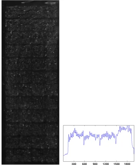
To do grid addressing, we need to segment the image into blocks, and then determine the grid within each block. The spots on a microarray are printed in a regular pattern: a microarray image will contain N×M blocks, where each block will contain p×q spots. Each of the image blocks in a microarray image is typically surrounded by regions void of any spots, and the blocks are arranged in a rigid pattern due to the printing process. For good quality microarray images, detecting the significant valleys in the vertical and horizontal projection profiles of the composite image, as was done in [9, 10], could already produce an accurate segmentation of the image blocks. However, when the image quality is not high, such a simple approach would not be robust enough since the significant valleys separating the blocks cannot be detected reliably. These two situations are depicted in Figs. 1 and 2. In Fig. 1, the significant valleys that correspond to the block boundaries can be observed in the vertical projection profile of a good quality image. In Fig. 2, the vertical projection profile of the composite image does not show any significant valleys separating the blocks.
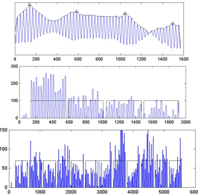
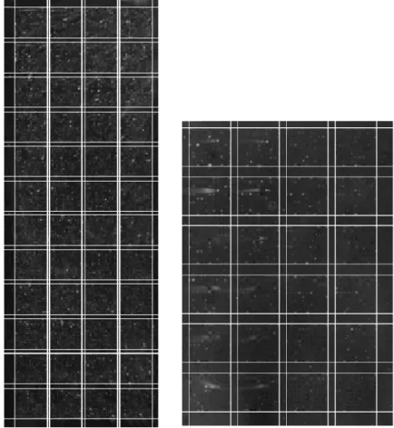
In our approach, we estimate a model of the block from the projection profiles and use this block model to find other “weaker” blocks. We start by thresholding the grayscale image to obtain a binary image. Then we generate the vertical and horizontal projection profiles from the binary image (note that the binary image can be divided into a number of non-overlapping subimages to generate a number of projection profiles). The projection profiles are then de-trended by morphologically filtered before we search for groups of well-defined spikes that are spaced regularly. The largest group of well-defined spikes is assumed to correspond to the true block and is used as a block model. To find the remaining weak blocks in the projection profiles, we use correlation processing, i.e. we perform cross correlation between the model and the processed projection profiles. By locating the peaks in the correlation signal envelop, we can identify the block locations robustly. Figures 3 and 4 show the correlation signal and the corresponding block segmentation result on the de-trended horizontal and vertical projection profiles for the image shown in Figs. 1 and 2. The block segmentation results are shown in the left and right panels of Fig. 5, respectively.
FIGURE 1. Left: Composite image. Right: vertical projection profile. Valleys that correspond to block boundaries can be clearly observed.
FIGURE 2. Left: Composite image. Right: vertical projection profile. No significant valleys separating the different blocks can be observed.
Figure 3. Correlation signal (top). The horizontal (middle) and vertical (bottom) block segmented de-trended projection profile for the image in Fig. 1. The block segmented image is shown in left panel of Fig. 5.
FIGURE 4. The horizontal (middle) and vertical (bottom) block segmented de-trended projection profile for the difficult image of Fig. 2. The block segmented image is shown in right panel of Fig. 5.
After image block segmentation, gridding is done within each image block. To generate the correct grid for each block, the location of high quality anchor spots is determined. We impose several criteria on good anchor spots: circular in shape, of appropriate size, with pixel intensity consistently higher than the background, and in locations agreeable with the printing configuration. These high quality anchor spots can then be used as anchors to infer the underlying grid structure.
FIGURE 5. Left: block segmentation result of image of Fig.1. Right: block segmentation result of image of Fig.2.
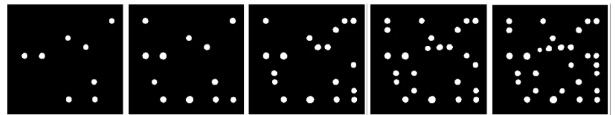
To detect the anchor spots, we perform a series of adaptive multi-level thresholding on the grayscale image. The purpose is such that strong and weak contrast spot patches (from which potential anchor spots are found) can be detected. We perform a series of morphological operations to each thresholded image to extract the anchor spots (see Fig. 6). The spot detection process for the sequence of images obeys a causality principle: once a spot is found in a higher threshold image, then any subsequent detection of spot at lower threshold image which overlaps with it in location is ignored. This ensures an adaptive detection of anchor spots of both strong and weak contrast in the composite image. It also enables better localization of the anchor spots since it allows the detection of spots at higher threshold value whenever possible.
The detected anchor spots are checked for size. Any anchor spot too large or too small is unreliable and is discarded. Then global rotation distortion is corrected by aligning the anchor spots vertically and horizontally. Since we typically have a number of anchor spots left, and they follow a rigid arrangement due to the printing configuration, any anchor spots that deviates too much from the grid assumed by the majority of the anchor spots are judged to be artifact and are removed. Fig. 7 shows the anchor spots and the final grid generated.
FIGURE 6. Successive anchor spot detection by adaptive thresholding and morphological processing. The threshold is decreased in a controlled manner to admit weaker and weaker spots from left to right.
FIGURE 7. Anchor spots detected (left) and final gridding (right)
SPOT SEGMENTATION
Spot segmentation is performed in each of the subregion defined by the grid. The segmentation involves finding a circle that separates out the spot, if present, from the image background. It can be divided into three major steps: (1) background equalization for intensity variation in the subregion, (2) optimum thresholding of the subregion, and finally, (3) finding the best-fit circle that segment out the spot.
Background equalization tries to remove any obvious intensity variation or ‘tilt’ in background intensity. Background intensity variation is obtained by sampling the intensity at the four corner of the subregion. Then a bilinear surface is estimated. The bilinear surface is subtracted from the original subregion to achieve background equalization.
When a spot is deemed to be present in a subregion, the intensity distribution of the pixels within the subregion is modeled using a 2-component Gaussian-Mixture Model (2-GMM). A spot is assumed present if an anchor spot is present, or when the ratio of the median intensity value of the tentative spot pixels and the median intensity value of the background pixels is larger than a preset value. We estimate the optimal model parameters by using the EM algorithm. After the model parameters are obtained, the optimum threshold is taken to be the value where the two Gaussian components intersect.
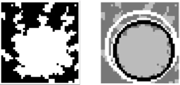
To segment the spot, we find the best-fit circle that enclosed the 2-GMM thresholded region. Given a binary image with foreground region and background region, the best-fit circle is defined to be the circle whose moment of inertia equals to that of the foreground region. An initial best-fit circle may enclose unwanted protrusions or artifacts. To exclude those erroneous regions, the computation of the best-fit circle is iterated, each time re-setting the foreground region not included in the previous best-fit circle to background region, until its radius and centroid remain constant between two successive iterations. Fig. 8 shows the foreground region
thresholded from a subregion (left) and a best-fit circle computed on the thresholded foreground region (right). The black circle is the final fit, which is obtained after 3 iterations of circle fitting. The best-fit circle has successfully captured the foreground region corresponding to the actual spot while excluding erroneous protrusions.
FIGURE 8. Best-fit circle computation for spot segmentation. Left: Thresholded region. Right: Best-fit circle iterated to exclude erroneous protrusions.
SPOT SEGMENTATION RESULTS
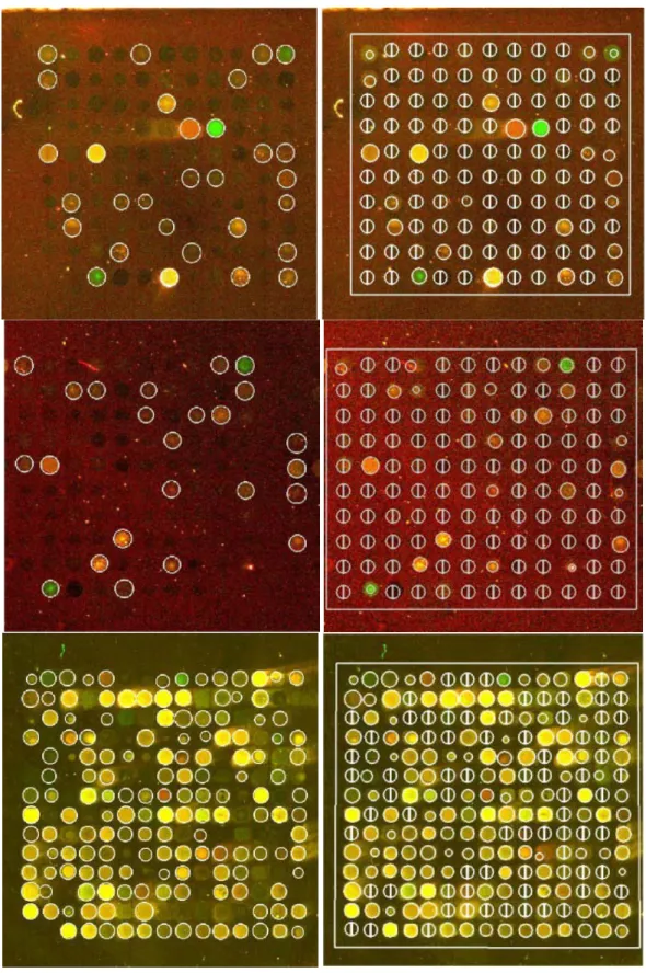
We present some segmentation results on both medium and high density cDNA microarray images. As a comparison, we also perform the segmentation using a commercial microarray segmentation package called GenePix3.0 [8]. Note that in GenePix3.0, it is necessary to specify the spot radius, the number of rows and columns, and also to align the grid template close to the actual spot manually to get a satisfactory result. In contrast, our algorithm estimates all the parameters automatically. Visual inspection of both sets of results in Fig. 9 reveals that the proposed algorithm has better performance than that of GenePix3.0, i.e., more spots are found and the spot size is more accurately determined. For GenePix3.0, the circle with a vertical bar signifies that spot is not found for that location. It was estimated that about 60-80% of the “not found” spots can be detected correctly by our algorithm, depending on the quality of the image. A quantitative evaluation was not performed since there is no ground truth available for real microarray images to conduct a meaningful and fair evaluation.
CONCLUSION
A novel spot segmentation algorithm is proposed for the automatic segmentation of spots from cDNA microarray images. The algorithm makes use of adaptive multi-level thresholding, shape and topological information via morphological processing, as well as Gaussian-Mixture intensity modeling to locate and segment out the spots. The algorithm consists of two major parts, (1) automatic grid addressing, and (2) spot segmentation. In contrast to many existing algorithms which require manual placement of a template grid close to the actual position and the input of spot parameters, our algorithm requires no manual operation from the user and is completely automated. Experimental results have verified that the proposed algorithm is robust and can handle cDNA microarray image of even very poor quality.
FIGURE 9. DNA Microarray spot segmentation results. Left: Proposed method. Right: GenePix Pro V3.0, where a circle with a vertical bar across it signifies that spot is not found at that location.
ACKNOWLEDGMENTS
This work is supported by a grant from the Hong Kong Research Grant Council (Project CityU 122506).
REFERENCES
1. M. Schena, D. Shalon, R.W. Davis, and P.O. Brown, Science 270, 467-470 (1995). 2. S.K. Moore, IEEE Spectrum, 54-60 (2001).
3. D.J. Lockhart, and E.A. Winzeler, Nature405, 827–846 (2000).
4. M. Steinfath, W. Wruck, H. Seidel, H. Lehrach, U. Radelof, and J. O’Brien, Bioinformatics 17(7), 634-641 (2001).
5. A.W.C. Liew, H. Yan, and M. Yang, Pattern Recognition 36(5), 1251-1254 (2003).
6. A.A. Ahmed, M. Vias, N. Gopalakrishna Iyer, C. Caldas, and J.D. Brenton, Nucleic Acids Research
32(5), e50 (2004).
7. L. Qin, L. Rueda, A. Ali, and A. Ngom, Applied Bioinformatics 4(1), 1-11 (2005). 8. GenePix Pro 3.0, Axon Instruments Inc. (2001)
9. JR.R. Hirata, J. Barrera, R.F. Hashimoto, and D.O. Dantas, Proceedings of XIV Brazilian Symposium on Computer Graphics and Image Processing 2001, 112 -119 (2001).
10. JR.R. Hirata, J. Barrera, R.F. Hashimoto, D.O. Dantas, and G.H. Esteves, Real-Time Imaging8(6), 491-505 (2002).