Single molecule diffusion in polymeric systems

(1)

i

Thesis presented in fulfilment of the requirements for the degree of Master of Science in Laser Physics in the Faculty of Science at

Stellenbosch University

Supervisor: Dr Gurthwin Bosman Co-supervisor: Prof Erich Rohwer

(2)

ii

DECLARATION

By submitting this thesis electronically, I declare that the entirety of the work contained therein is my own, original work, that I am the sole author thereof (save to the extent explicitly otherwise stated), that reproduction and publication thereof by Stellenbosch University will not infringe any third party rights and that I have not previously in its entirety or in part submitted it for obtaining any qualification. April 2019

(3)

iii

ACKNOWLEDGEMENTS

I thank the Lord God Almighty for granting this opportunity to me to undertake studies at Stellenbosch University and the strength to be able to complete this project.

I would like to express my deepest appreciation to my supervisors Dr G. Bosman and Prof E. Rohwer for encouraging me, teaching to work very hard and guiding me throughout the project. I would have never been able to complete this project without both their excellent guidance and patience as they helped me in improving my skills in experimental laser physics. I would like to thank Prof E.G Rohwer for allowing me to join the laser research institute (LRI), the great environment to undertake the project and for granting to me the SARCHI bursary to undertake studies with the physics department and thank ALC Scholarship grant for financial support. My sincere appreciation for the financial funding. I thank my family and close friends for always believing in me and supporting me always.

Lastly but not least, I thank the LRI team at Stellenbosch University for their warm welcome to me and Dina Ratsimandresy for assistance with coding and image processing techniques.

(4)

iv

DEDICATIONS

To my son, Melchizedek, may you always strive to attain you dreams and goals.

(5)

v

ABSTRACT

Single molecule diffusion in polymeric systems

Charmaine Sibanda

Department of Physics, University of Stellenbosch,

Private Bag X1, Matieland 7602, South Africa.

Thesis: MSc

April

2019

The dynamics of thin polymeric systems were studied in this research work using the diffusion of single fluorescent molecules observed by single molecule fluorescence microscopy. A wide field single fluorescence microscopy setup was designed together with a custom-built heating stage to study the nano-environments of two different polymeric systems and how these systems are affected by a change in temperature. The designed optical setup achieved a localization precision of 20 nm which further enabled the tracking of single molecules embedded in polymeric systems. The position trajectories of the single molecules in the polymer matrices are used to calculate the motion of the single molecules from which the diffusion coefficient data is extracted. The distribution of the diffusion coefficients is a consequence of the microscopic dynamics of the polymeric systems coupled to the probe molecules. The fluorescence intensity pattern analysis of the single molecules is also used as reporters of the nano-environment of thin polymeric films.

(6)

vi

UITTREKSEL

Die dinamika van dun polimeerstelsels is bestudeer in hierdie navorsingswerk met behulp van die diffusie van enkele fluoreserende molekules waargeneem deur enkelmolekule fluoressensie mikroskopie. 'n Wye veld enkel fluoressensie mikroskopie opstelling tesame met 'n toepaslike monster verwarmingstoestel is ontwerp om die nano-omgewings van twee verskillende polimeerstelsels te bestudeer onder die geringste temperatuurverandering. Die optiese opstelling het 'n enkelmolekuul lokaliserings-presisie van 20 nm behaal. Hierdie aansienlike presisie het toegelaat dat die posisies van die enkele molekules in die polimeermatrikse gebruik word om die diffusie-koëffisient van die enkele molekules te bereken. Die verspreiding van die diffusie koëffisiënte is 'n gevolg van die mikroskopiese dinamika van die polimeerstelsels gekoppel aan die molekules. Die enkelmolekuul fluoressensie intensiteit word ook ontleed en daar word getoon dat daar ‘n definitiewe monster afhanklikeheid bestaan.

(7)

vii

Table of figures

Figure 1. Formation of polystyrene through vinyl polymerization, which is an example of addition polymerization. the carbon double bond is broken by the free radical and a polystyrene polymer is formed. Image taken from [7]. _________3 Figure 2. Condensation polymerization of a carboxylic and amine monomer to produce a polyamide Nylon. _________________________________________4 Figure 3. Difference in physical chain segment structure of polymers. Amorphous polymer chain segments are disarranged, and semi-crystalline polymer chain segments have some degree of order within the polymer chain, image adapted from [8]. _________________________________________________________4 Figure 4. Effect of temperature on amorphous and semi-crystalline polymer chain segments. At low temperatures both chain segments are brittle and immobile, as temperature is increased, a region where polymer segments are rubbery, and mobile is reached called the glass transition temperature. This temperature region affects the processing and application of polymers. Semi-crystalline polymers have a melting temperature due to the ordered nature of the chain structure and as a result have a narrow processing range. Amorphous polymers have no definite melting temperature a direct consequence of the disarranged chain structure and thus have a broad processing range. Image adapted from [10]. ____________________________________________________________6 Figure 5. Typical schematic showing non-Arrhenius α-relaxation process and Arrhenius β-relaxation process as function of inverse temperature. Deviation from the Arrhenius behavior of the alpha process is due to the heterogeneities arising from the motion of the main chain long-range motion that is frozen in the glassy state to result in slow dynamics. ________________________________8 Figure 6. A graph plotted from simulated results using equation (v), with Tg = 56

ᵒC. As the temperature is decreased towards the glass transition temperature, the viscosity of the polymer is expected to increase. However, as the glass transition is approached (< 65 ᵒC), viscosity increases by orders of magnitude due to heterogeneities associated with α-relaxation processes and for temperatures at and below the glass transition temperature, the free volume theory fails to explain effects of heterogeneous dynamics. ___________________________ 10 Figure 7. A Jablonski diagram is used to describe fluorescence emission. The molecule absorbs energy from ground state S₀ and is excited to first excited state S₁, the excited molecule collides with surrounding molecules and loses energy

(10)

x

non-radiatively before falling to S₀ emitting a photon in the form of fluorescence. The molecule can undergo nonradiative transitions through intersystem crossing (ISC) due to singlet-triplet spin-orbit coupling. From the lowest excited triplet state the molecule can either return to singlet ground state through phosphorescence or undergo a permanent change due to photo dynamics interactions rendering its ability to fluoresce thereby becoming going into a photobleached state. _____________________________________________ 12 Figure 8. A typical wide field fluorescence microscopy set up, the sample area imaged is large and excitation is from a collimated laser beam that is focused on the back-focal plane of the objective. The fluorescence emission from the sample is collected through the same objective and is separated from the incident excitation laser beam using a dichroic mirror and suitable filters and finally detected using a scientific CCD camera Image taken from [14]. ___________ 13 Figure 9. (a) Experimental setup that was used for imaging single molecules embedded in a thin polymer film sample. ND– neutral density filters, RM– reflecting mirror, WP- quarter waveplate. AL – aspherical lens, SMF – single mode fiber, PL – pre-focusing lens, DBS- dichroic beam splitter, Obj- microscope objective, NF- notch filter, FM- flip mirror, AD- achromatic doublet, BF- bandpass filter. (b) Graph showing how stable the incident light was after coupling it through a single mode fiber, coupling efficiency was calculated to be 40 %. _ 17 Figure 10. (a) Experimental set-up to produce circularly polarized light through the insertion of a quarter waveplate. A linear polarizer was also introduced and was rotated in front of a power meter used to check the intensity of the polarized light. ND- neutral density filters, RM- reflecting mirror, WP- quarter waveplate, AL- aspherical lens, SMF- single mode fiber, CL- collimating lens, LP- linear polarizer, PM- power meter. (b) Graph shows the power intensity stability measured as the linear polarizer was rotated. From the graph it can be observed that the power intensity remained constant as the angle of rotation, thus the indicating that the polarization state of the excitation light was successfully changed to circular. ______________________________________________ 19 Figure 11. The thickness of polystyrene films is determined using the ratio of absorbance of liquid polystyrene solution (a) and that of a solid polystyrene film spin-coated on a MgF slide (b), were the absorbance is proportional to the density of the material and its length/thickness. The absorbance of the liquid polystyrene liquid solution was measured to be 0.5 and that of the polystyrene film 0.1. _ 22

(11)

xi

Figure 12.Image on the left shows the grayscale image of the calibration grid and on the right, the intensity profile resulting from cutting along a horizontal line drawn across the grid using ImageJ. 270 pixels counted on camera represents 10µm in real space dimensions of the grid imaged. _____________________ 23 Figure 13.Localization precision of single fluorescent perylene dye molecules embedded in polystyrene (circled in red) were imaged over 100 frames, camera exposure time of 500 ms and at a temperature of 17 ᵒC. The loci of the individual emitters were used to calculate the localization precision in both the X σ = 5 nm (bottom left) and Y σ = 6 nm (bottom right) directions. The deviation in the localization precision is a result of the polymer chain nano-environment which is known to be complex as was studied by Tomczak et al [34]. ______________ 24 Figure 14. Image on the left shows three 2 μm fluorescent microspheres acquired over 30 mins and used to characterize the microscope stage drift dynamics. The stage drift dynamics are characterized using the diffusion coefficient of the microspheres extracted from the slope of the MSD graph (right).__________ 25 Figure 15. Heating setup used for heating polymer samples. The mechanisms employed to heat the samples is Joule heating, were a current is passed through the resistive ITO cover slide which then heats up as the charge carriers interact, collide and scatter from the ITO atomic ions, thereby producing thermal energy. ______________________________________________________________ 27 Figure 16. The graph shows that the heat energy is directly proportional to the voltage, current and thus an increase in voltage and current results in an increase in thermal heat energy. ___________________________________________ 27 Figure 17.a) The structure of the PBI dye molecule that was embedded in two different polymer environments. The polymers that were used in this research work are Pibma with glass transition temperature of 55 ᵒC (b) and Ps with a lower glass transition temperature of 100 ᵒC (c). ____________________________ 29 Figure 18. Image sequences of PBI dye molecules embedded in a Pibma (a) and Ps (b) film at an exposure time of 200 ms and 18.5 ᵒ C. A notable difference between the two polymers on the fluorescence emission of PBI is the number of observable single molecules and the photobleaching of PBI molecules in Ps film. ______________________________________________________________ 30 Figure 19. (a) Insert show the typical blinking behavior of single molecules in the thin polymer films. (b) Influence of polymer environment to single fluorescent molecules emission. From the Ps film, the individual fluorescent probes were noted to photo blink and most photo bleaching as a function of time. The Pibma

(12)

xii

film showed the number of fluorescent probes to relatively stay the same across each image frame and photo blinking was observed. ___________________ 31 Figure 20. Narrow distributions of the diffusion coefficients of PBI in Pibma (on the left-hand side) and Ps (on the right-hand side) thin films imaged at 18.5 ᵒC show that far below the glass transition temperature the polymer chains and segments are rigid. The rigidity of the polymer chains and segments means reduced free volume distributions in the polymer or the caging effects that hinders motion of small probe molecules within the polymer film at very low temperatures below Tg [37]. _______________________________________ 32 Figure 21. Static heterogeneities of polystyrene were studied by observing the photo physical changes of PBI in air as a function of temperature. Photo blinking and photo bleaching of single molecules was observed with increased photo bleaching for PBI in air. ___________________________________________ 33 Figure 22. Static heterogeneities of polystyrene were studied by observing the photo physical changes of PBI in a Ps film as a function of temperature. The number of observed single PBI molecules in a Ps film increase as compared to single PBI molecules on a plain ITO cover slide. ________________________ 34 Figure 23.The effective photo bleaching rate reduces as temperature is increased for PBI in Ps film 23 ms to 18 ms for 18.5 ᵒC and 43.5 ᵒC respectively (on the left-hand side). The effective photo bleaching rate PBI in air is approximately constant ~8 ms for both temperatures (on the right-hand side). The effective photo bleaching rate was extracted from the slope of the linear fit graph. ________ 35 Figure 24. The average intensity count for PBI in Ps film was lower than that of PBI in air (top graph). Fluctuations in the average intensity trace of PBI as the temperature is increased (left) is attributed to the static heterogeneities within the polymer film that include different amounts of free volume distribution, enhanced surface interfaces because of the thin film and local density fluctuations of the polymer chain segment structure. The excited PBI probe molecule fluorescence emission was influenced by the interactions between the polymer film and the amount of oxygen that could diffuse through the polymeric film as the temperature is increased these interactions also increased and contributed to the photo bleaching of PBI dye molecules in the Ps film (right). 36 Figure 25. a) Zoomed in image of individual fluorescent molecule, the red pattern is the trajectory length indicating movement of the molecule. b) the loci position shifts from the initial start coordinate illustrate how the molecule moved in the x

(13)

xiii

and y directions, movement is isotropic from the histogram distribution and can be assumed to be Brownian. _______________________________________ 38 Figure 26. By tracking the molecule movement in the polymer, the mean square displacement is extracted at each time lag of 200 ms and from which the slope of the MSD plot gives the diffusion coefficient of an individual PBI in Pibma film. ______________________________________________________________ 39 Figure 27. Diffusion coefficients of PBI in Pibma at four different temperature ranges indicates that as the temperature is increased the standard deviation of the diffusion coefficients increases due to the heterogeneous cooperatively rearranging regions. As the Tg for Pibma is slowly approached the translational diffusion of the PBI reduced. _______________________________________ 40 Figure 28. The Vogel-Fulcher law fails to describe the viscosity temperature dependence of the diffusion coefficients of PBI molecules in Pibma due to heterogeneities in the thin film as shown in the plot of In(D) against temperature (left). A plot of the standard deviation of the diffusion coefficients illustrates the increase of heterogeneities as the temperature is increased until the approach of Tg of Pibma (55 ᵒC), where the translational diffusion processes are slowed down (right). _________________________________________________________ 41 Figure 29. Cooperatively rearranging regions within a polymer have been said to cause a caging effect on probe molecules embedded in the polymer film. At low temperatures below the Tg of a polymer film, each size of the CRRs is large and the number of the polymer segments large and motion of the regions is through vibrations which are coupled to the probe molecules and the relaxation process associated with this motion is the β-relaxation. As the temperature is increased towards Tg, the size CRRs reduces and the number of polymer segments within the CRRs reduces hence breaking the caging effect on the tracer molecules [25], [34], [50]. The cage breaking effect enhances the diffusion of the probe molecules within the polymer film and the relaxation process associated with this motion is the α-relaxation process. __________________________________________ 42 Figure 30. Enhanced surface interfacial interactions cause heterogeneities that contribute to Tg shifts in thin polymer samples as compared to their bulk counterparts [53], [54]. The reduced polymer chain density at the surface assists the diffusion motion of individual fluorescent tracers across the film, however the local density distribution of amorphous polymer chains is random thus the motion of the probe molecules is also expected to be inhomogeneous. _____ 43

(14)

xiv

Figure 31. Decreasing average fluorescence intensity of PBI single molecules in Pibma as temperature was increased was observed. ____________________ 44

(15)

1

Chapter 1: Introduction

Thin polymeric systems have become very important materials due to their unique adjustable physical properties. This is evident through reports that that indicated the rise in polymer production which was pegged at 8.3 billion tonnes in 2017 [1]. The physical properties of thin films are important for different industrial sectors such as the coating and adhesives sector, biomaterials sector amongst many others. Temperature is known to affect the physical properties of thin polymeric systems which are a consequence of microscopic dynamics of the polymers and affect the application of the polymer through its service temperature. One such unique property of thin polymeric systems is the reduction of their service temperature in comparison to a thick film of the same material. Bulk polymer research studies have been vastly conducted many decades before, however thin polymeric system dynamics, in particular the glass transition shifts are still not yet fully understood [2]. Hence further need arises to employ experimental and theoretical tools in understanding thin polymeric film systems.

The technique that was employed in this work to study the dynamics of thin polymeric systems was single molecule fluorescence microscopy. Advantages of using this technique include direct observation of single molecules thereby eliminating the need for ensemble averaging which obscures complex properties in bulk measurements [3] and the sensitivity of fluorescence to minute changes in the probe environment means that fluorescent probes become a natural choice as a molecular reporter of thin polymeric system. By tracking the single molecule position through diffusion processes and analyzing its fluorescence intensity in a polymeric system enables us to study the microscopic dynamics of the polymeric systems.

The work in this research project covers discussions on definitions of polymers and how they are made and the effect of temperature and glass transition temperature of polymeric systems. Further information is given in Chapter 2 on bulk polymer models and how these models have been used in trying to explain heterogeneities in polymers and application of single molecule fluorescence microscopy to polymer research is introduced in the same chapter. The design of the optical setup that was used and its characterization is given in Chapter 3 that enabled the study of diffusion of single molecules in polymeric systems. The results and discussions of the measurements of single molecule motions and fluorescence emission trajectories observed when the dye molecules were embedded in different polymeric systems are analyzed and the causes of diffusion processes related to microscopic dynamics of the polymeric systems are covered in Chapter 4.

(16)

2

Chapter 2: Literature review

Polymers are materials composed of high relative molecular mass built from repeat units of low relative molecular mass. World production of polymers has been pegged at over 8.3 billion tonnes in 2017 which in turn has also increased the necessity for sustainable options for polymer production, recycling and waste management [1]. The high demand of polymers has made them become one of the most important in the biomedical sectors related to biocompatibility of medical implants, drug delivery system and industrial sector related to protective and functional coatings [4]. The photophysics and photochemistry in polymer research has been central areas of interest in understanding the structure and dynamics of polymers. These materials have shown interesting and unique physical properties that change drastically such as viscosity and thermal expansion below, near and above the glass transition temperature which originate from complicated relaxation processes of polymer chains [5].

However, these unique properties have not yet been fully understood despite theoretical and experimental studies over the past decades. Hence the need to further study the temperature dependence of the physical properties of polymers as they are of high crucial importance for various applications. Different experimental methods have been used to try understanding the nano-environment of polymers. One of these methods also used in this research and described in greater detail in this chapter, is single molecule fluorescence microscopy. It is a powerful imaging technique that enables the direct observation of single fluorescent molecules in their nano-environment. In this chapter more, detail is given on the definition of a polymer and how they are formed, then focus on temperature dependence of polymers, the consequence of these dependences to polymer chains and define what the glass transition temperature is. Also covered in this section is the models from past literature that have been used to try understanding the polymer nano-environment in different temperature ranges and finally why the use of single molecule fluorescence microscopy was chosen as a preferential technique about polymer dynamics.

(17)

3

2.1 Polymers

Polymers are macromolecules formed through polymerization and are composed of a basic repeat unit called a monomer [6].

The two main types of polymerization are addition/chain polymerization and condensation/step reaction polymerization.

Addition/Chain reaction polymerization

Addition polymerization is a three-step process. The process begins with initiation, then propagation and ends with termination.

Initiation- a double bonded carbon monomer reacts with a catalyst usually a free radical species. The double bond is broken and the monomer bonds to the free radical species an example is the formation of polystyrene where the styrene monomer reacts with a free radical to form polystyrene (Figure 1). Propagation- in this step the styrene monomer units are added sequentially to the reactive chain molecule. The reactive site is transferred to each styrene monomer as it is linked to the chain which gets longer and longer.

Termination- this takes place when another free radical meets the ends of the long growing polymer chain. The free radical terminates the chain by linking with the reactive propagating polymer chain thus producing a complete polymer chain.

Figure 1. Formation of polystyrene through vinyl polymerization, which is an example of addition polymerization. the carbon double bond is broken by the free radical and a polystyrene polymer is formed. Image taken from [7].

Condensation polymerization

Condensation polymerization involves two different types of monomers that react through stepwise intermolecular chemical reactions to form a polymer chain, also a by-product is formed usually water

(18)

4

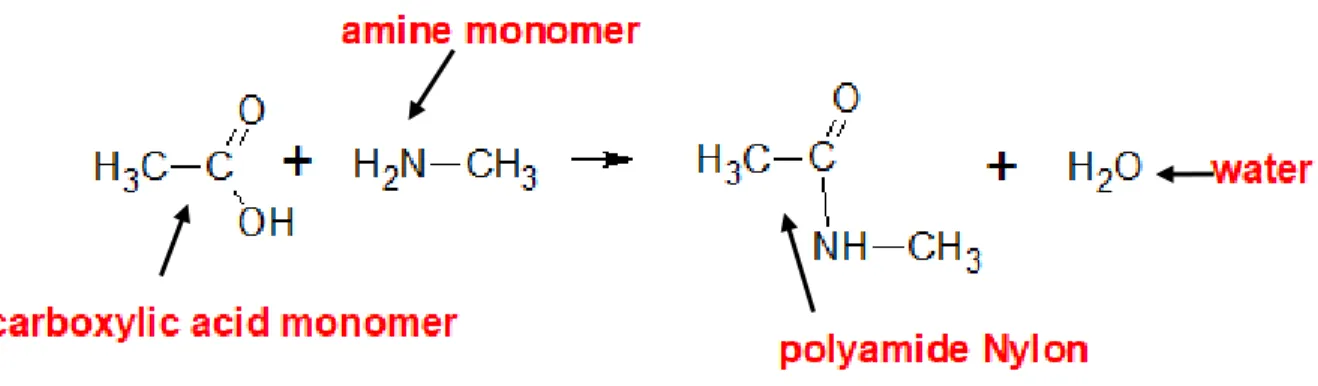
or methanol. In the example given below, a carboxylic acid monomer and an amine monomer join in an amide linkage to form a polyamide Nylon and a water molecule is removed (Figure 2).

Figure 2. Condensation polymerization of a carboxylic and amine monomer to produce a polyamide Nylon.

2.1.1 Polymer physical structure

Polymer chain segments can exist in two distinct physical structures. These segments are either semi-crystalline or amorphous in form.

Amorphous polymers have a disarranged chain structure and semi-crystalline polymers have some degree of ordered arrangement of the chain segments. The difference in molecular segments between an amorphous chain structure which is entangled and randomly arranged compared to a semi-crystalline chain structure which shows some ordered arrangement of the chain segments (Figure 3).

Figure 3. Difference in physical chain segment structure of polymers. Amorphous polymer chain segments are disarranged, and semi-crystalline polymer chain segments have some degree of order within the polymer chain, image adapted from [8].

(19)

5

2.2 Effect of temperature in polymers

The disarranged order of chain segments in amorphous polymers prevents them from having a definite melting temperature, in contrast the partially ordered arrangements of semi-crystalline chain segments gives this type of polymers a melting temperature.

At lower temperatures, the chain segments of polymers are often brittle and immobile, as the temperature is increased the molecular chain mobility is increased and at even higher temperatures the polymer chains flow as highly viscous liquids and form a visco-elastic material.

2.2.1 Glass Transition Temperature (Tg)

This is the temperature region where immobile polymer chain segments slowly soften to a rubbery disordered glassy state and a viscosity of 10¹² Pascal-seconds (Pa.s) is reached, as the temperature is increased [9]. The glass transition can also be defined as the temperature where the average molecular relaxation time of the polymer sample material is approximately 100 seconds depending on the heating and cooling rates. The contrast in molecular chain motion between amorphous and semi-crystalline polymers as a function of temperature, below the glass transition temperature both chain segments are immobile, an increase in temperature sees an increase in chain mobility and flexibility, where the polymer undergoes a glass-rubber transition known as the glass transition temperature. This region is also known as the service region of polymers and directly influences the processing and application of polymers [10]. Using calorimetry experimental methods to investigate the response of polymers to heat results in a plot of heat flow against temperature. An increase in temperature from the heat flow versus temperature plot indicates a dip due to change in heat capacity that is reached after the plateau for semi-crystalline polymer chain segments, this dip marks the melting temperature for this polymer. For amorphous polymers, the chain segments flow as a visco-elastic material and show no definite melting temperature (Figure 4).

(20)

6

Figure 4. Effect of temperature on amorphous and semi-crystalline polymer chain segments. At low temperatures both chain segments are brittle and immobile, as temperature is increased, a region where polymer segments are rubbery, and mobile is reached called the glass transition temperature. This temperature region affects the processing and application of polymers. Semi-crystalline polymers have a melting temperature due to the ordered nature of the chain structure and as a result have a narrow processing range. Amorphous polymers have no definite melting temperature a direct consequence of the disarranged chain structure and thus have a broad processing range. Image adapted from [10].

2.2.2 Thin polymer film dynamics below and above glass transition

The physical properties of thin films are important for different applications such as coatings, adhesives, biomaterials amongst many others [11]–[13]. To be able to design a specific surface, there is need to be able to control film thickness, which in turn reveals different degrees of molecular motion for different thicknesses [14]. Thin polymer films have shown different properties at their interfaces as compared to thick films. One major difference is the reduction of Tgat the surface for thin films as compared to thick

films, that is bulk Tg for the same polymer material. This decrease in Tg in thin films is attributed to

enhanced surface mobility of the molecular chains due to a large surface to volume ratio of the nanometer scale films [15].

These associated changes in Tg due to enhanced surface mobility directly affect polymer dynamics.

Different approaches have been used to directly study polymer dynamics such as the relaxation processes in polymers. At high temperatures, polymer chain segments have fast motions and very short relaxation time scales and at low temperatures, the molecular chain mobility decreases as the relaxation time scale

(21)

7

increases such that the chain segments are frozen before the system is in thermodynamic equilibrium [16]. The dynamics of amorphous polymers at temperatures below and near Tg are heterogeneous and

above the Tg the dynamics are homogeneous. Heterogeneous dynamics show some regions of the

polymer environment with high molecular mobilities whilst adjoining regions can exhibit slow molecular mobilities [17].The two main relaxation processes that have been observed are alpha-relaxation and beta-relaxation processes [9]. The beta-relaxation time refers to the time it takes for the polymer chains to respond to temperature changes.

Alpha relaxation- This is the primary relaxation process in most amorphous polymers and corresponds to structural relaxation or main chain long range motion of the entire polymer chain connected to viscous flow [18]. Alpha relaxation process shows a strong temperature dependence and exhibits strong spatial heterogeneities [9]. The temperature dependence of viscosity involving main chain long range motion, that is alpha relaxation, in a bulk polymer that has been cooled down from high temperatures show non-Arrhenius behavior known as the Vogel-Fulcher law [9]:

η(T) ∝ exp

B

T−T_VFT_(i)

The Vogel-Fulcher law implies that at high temperatures above the glass transition, the viscosity of the polymer chain melt is low, and the polymer melt flows with less frictional resistance. As the polymer melt is cooled down, the viscosity of the chains gradually increases and at the glass transition temperature the viscosity increases by orders of magnitude and the polymer main chain motion become very slow compared with the experimental time scales, that is viscosity of 10¹² Pa.s is reached and relaxation time scale of 100 s.

Beta relaxation – this is the secondary relaxation process which is caused by local motion of polymer segments, small scale backbone fluctuations from main chain rotations, vibrations associated with motion of polymer side groups rotating around bonds linked to main chains and it shows very short time scales and Arrhenius temperature dependence [19]. Arrhenius temperature dependence equation (ii) and an Arrhenius plot can be drawn by taking the natural logarithm of equation (ii), which yields the same form as that for the equation of a straight line, whose gradient gives the activation energy parameter and the intercept gives the pre-exponential factor. From the Arrhenius plot, the alpha process diverges as it approached the Tg because of the long-time scales from the main polymer chain with long range motions

coupled with orders of magnitude of viscosity (Figure 5).

τ ∝ exp

E

k_bT_(ii)

B – is the activation energy equivalent parameter and Tvft– Vogel Fulcher Tammann temperature

which is the ideal glass transition temperature, typically 50 ᵒC below the glass transition temperature, that marks the start of discontinuities in some thermodynamics quantities.

(22)

8

Figure 5. Typical schematic showing non-Arrhenius α-relaxation process and Arrhenius β-relaxation process as function of inverse temperature. Deviation from the Arrhenius behavior of the alpha process is due to the heterogeneities arising from the motion of the main chain long-range motion that is frozen in the glassy state to result in slow dynamics.

2.3 Model/s for glass transition theories

2.3.1 Free volume theory

In this theory the molecules in a polymer melt state occupy much of the melt’s volume, partly as molecules that make up the monomers and partly as inaccessible volume that is blocked from access by steric factors. The remaining small fraction of volume is referred to as ‘free’ volume and is used for molecular motion [20].

For a polymer melt that is cooled from high temperature, the density is expected to increase as the free volume decreases, consequently the molecular motion is hindered, and the viscosity increases. According to Doolittle [21] the viscosity of a polymer liquid is related to the fractional free volume by equation (iii):

η~ exp

bV_t

V_f_(iii)

b - is an empirical unit-less constant. Vt and Vf is the total volume and fractional free volume

respectively. At higher temperatures above the glass transition, the polymer chains occupy a large total volume, free volume increases also, and the viscosity reduces as the polymer melt flows easily. As the temperature is reduced, the free volume occupied by the polymer chains is reduced and the motion of the polymer chains is coupled to chain segments that move cooperatively and viscosity increases.

(23)

9

Doolittle made some assumptions to his equation that the activation energy for flow is inversely proportional to the fractional free volume Vf and the free volume has a linear temperature dependence

above Tg given below:

Vf ∝ (T − Tg) (iv)

The Doolittle equation can be combined with the assumption of linear temperature dependence of fractional free volume to get the modified Doolittle equation that relates the viscoelastic properties to the glass transition temperature.

η ∝ exp(

b Vt

(T − Tg))_(v)

If the alpha relaxation process is being probed, then the viscosity is expected to increase by orders of magnitude as the glass transition temperature is approached as illustrated in Figure 6, showing simulated graph for equation (v) and polymer main chain motion is arrested. However, the free volume theory fails to explain dynamics observed below the Tg temperature for glassy polymers. The free volume values were

extrapolated from differences in volume between a polymer that has been cooled below its Tg (that is in

its glassy state) and a polymer melt cooled above its Tg ( melt state) and large discrepancies between

reported values for the value of free volume at glass transition have been reported ranging from 2.5-11.3% [22], thus indicating the need for further studies of amorphous polymer microstructure. The free volume theory is a statistical average quantity obtained from equilibrium states and moving towards glass transition from high temperatures, the state of the polymer is not in equilibrium state as a result using free volume theory in this temperature region obscures effects of heterogeneous dynamics. Studies have shown that there is no correlation between the free volume and the glass transition, that is, the glass transition of glassy polymers is not caused by the absence of free volume [23]. Therefore, a more direct knowledge of the microstructure of amorphous polymers is needed to verify the main assumptions made in the free volume theory and quantitative aspects of the free volume distribution and dynamics remain unknown.

(24)

10

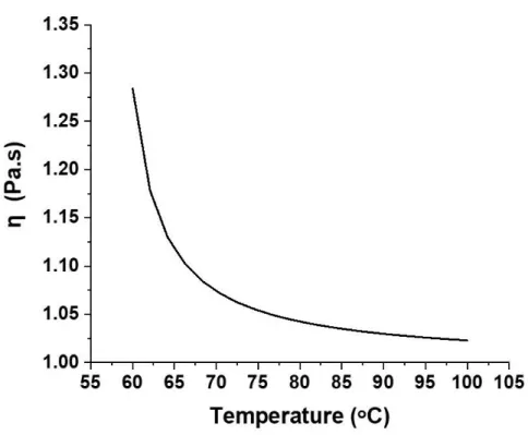
Figure 6. A graph plotted from simulated results using equation (v), with Tg = 56 ᵒC. As the temperature is decreased towards the glass transition temperature, the viscosity of the polymer is expected to increase. However, as the glass transition is approached (< 65 ᵒC), viscosity increases by orders of magnitude due to

heterogeneities associated with α-relaxation processes and for temperatures at and below the glass transition temperature, the free volume theory fails to explain effects of heterogeneous dynamics.

2.3.2 Adam-Gibbs molecular-kinetic theory

The Adam-Gibbs theory describes the temperature dependence of relaxation time processes of polymers in terms of the disappearance of the configurational entropy of the cooperatively rearranging regions (CRR) [24]. The main assumption of this theory is that a polymer melt has several segments that cooperatively rearrange. The movement of the independent CRRs changes the configuration of the polymer system and this motion, determined via the diffusion constant given by equation (vi), is related to the configurational entropy Scof the polymer system given by equation (vii) and temperature T [25].

D ∝ expTSc−B_(vi)

Sc = kbInWc (vii)

(25)

11

Each polymer chain segment is composed of monomers that rearrange themselves independently of its environment. At low temperatures the mobility of the polymer chain segment is very slow and individual chain molecular motion is absent, instead adjoining chain segments move by cooperative rearranging. As temperature is further reduced towards the glass transition temperature, the size of the cooperative rearranging regions CRR becomes larger and the configurational entropy of the system decreases, and this leads to an increase in viscosity. At even lower temperatures the configurational entropy becomes zero and the system exhibits one cooperatively relaxing region with no further freedom to rearrange its structure [26].

At the molecular level the dependence of the viscosity/relaxation time is given by equation (viii), where the viscosity and relaxation time depend on the number of chain segments which must move within the cooperatively rearranging regions.

η(T), τ(T) = Cexp

z∗∆μ

kbT (viii)

Despite the success of the Adam-Gibbs theory of being able relate the microscopic dynamics of the CRRs to macroscopic configurational entropy of glassy polymers, it does not predict the size of the CRRs nor the explicit dependence of the CRRs to temperature.

2.4 Fluorescence imaging

This is the imaging of fluorescing molecules using a fluorescence microscope. A fluorophore1_{can either}

be in the singlet ground state or once radiated by electromagnetic radiation within the absorption spectrum of the fluorophore is excited to the first singlet state. Typically, the fluorescence of a molecule is described using a Jablonski diagram (Figure 7). The excitation of a fluorophore as it absorbs energy from the singlet ground state and reaches higher vibrational levels of the first excited singlet state. It then loses its excess of vibrational energy and relaxes to the lowest vibrational level of the excited state. The fluorophore continues to lose energy until the lowest vibrational level of the first excited state. From the lowest vibrational level of the first excited state, it can relax to any of the vibrational levels of the ground state and emits a photon in the process as fluorescence.

The excited molecule has a chance to undergo intersystem crossing to the excited triplet state due to spin- orbit coupling that causes the single molecule to flip its spin and end up on the triplet state. If the lowest triplet state remains occupied, the transition from the singlet ground state to the first excited singlet state does not occur and fluorescence emission is temporarily interrupted, and the molecule is said to be in a dark state. The molecule relaxes back to the singlet ground state from the triplet excited state through phosphorescence. After decaying from the triplet state to the singlet ground state, the molecule starts to

1_{Fluorophores are typically polyaromatic hydrocarbon molecules that re-emit light upon optical excitation [57].} η (T), τ(T) is the viscosity and structural relaxation time at a given temperature T respectively, C is a constant, z* is the number of monomer units contained in the smallest region capable of rearranging, ∆μ is the energy barrier for the chain segments to move, kbis the Boltzmann constant.

(26)

12

fluoresce, and this phenomenon is called photo blinking and it is a reversible process. Fluorescence photons are emitted in bunches and separated by photo blinking periods, which occur when the molecule is in the triplet state. The triplet state lifetimes are dependent on the concentration of molecular oxygen. Fluorescence emitted by all fluorescent dyes fades during observation and this involves a photo chemical modification of the dye and results in irreversible ability of the dye molecule to fluoresce. A molecule in the excited triplet state can undergo a permanent change that renders its ability to fluoresce, thereby becoming a photo bleached molecule. The main cause of photo bleaching of fluorescent single molecules is due to photo dynamic interactions between the excited fluorophores and molecular oxygen in its triplet ground state.

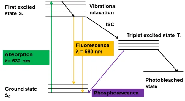
Figure 7. A Jablonski diagram is used to describe fluorescence emission. The molecule absorbs energy from ground state S₀ and is excited to first excited state S₁, the excited molecule collides with surrounding molecules and loses energy non-radiatively before falling to S₀ emitting a photon in the form of fluorescence. The molecule can undergo nonradiative transitions through intersystem crossing (ISC) due to singlet-triplet spin-orbit coupling. From the lowest excited triplet state the molecule can either return to singlet ground state through phosphorescence or undergo a permanent change due to photo dynamics interactions rendering its ability to fluoresce thereby becoming going into a photobleached state.

Using spatially resolved imaging this fluorescence can be imaged using a microscope. One such microscope that is used to image fluorescence is wide field fluorescence microscopy. The microscope set up is designed in such a way that allows the separation of the intense optical excitation from the relatively weak fluorescence using appropriate dichroic mirrors [27]. A typical wide field fluorescence microscopy set up comprises a laser beam used as the exciting incident light, which is collimated and focused at the back-focal plane of high numerical aperture objective to achieve a uniform field of illumination for the sample (Figure 8). The emission is then collected via the same objective and passes through the tube lens and filters to separate the excitation light and imaged onto an imaging sensor (CCD – charged couple device or CMOS – complementary metal-oxide semiconductor).

(27)

13

Figure 8. A typical wide field fluorescence microscopy set up, the sample area imaged is large and excitation is from a collimated laser beam that is focused on the back-focal plane of the objective. The fluorescence emission from the sample is collected through the same objective and is separated from the incident excitation laser beam using a dichroic mirror and suitable filters and finally detected using a scientific CCD camera Image taken from [14].

Some parameters that can be extracted from fluorescence microscopy are: i) Fluorescence intensity

ii) Molecule position iii) Fluorescence lifetime

The advantages that have made fluorescence microscopy especially single molecule resolved fluorescence an invaluable imaging technique which allows the observation of smaller and smaller objects with great optical resolution that is below the diffraction limit include:

i) High sensitivity of fluorescence to changes in fluorophore environment thus can be applied in different research fields such as studying polymer dynamics in their nano-environment. ii) Single molecule detection has enabled the ability to track and manipulate the individual

emitters. This technique of being able to view one single emitter at a time eliminates the tendency of ensemble averaging.

(28)

14

iii) Another advantage is that fluorescence lifetimes are very sensitive to the properties and changes of the probe molecule environment, as a result this means fluorescent probes become a natural choice as molecular level reporter of nano-environments.

2.5 Single molecule fluorescence microscopy- An application to polymer research

Different experimental methods have been used to try understanding the glass transition temperature and polymer nano-environment dynamics using dielectric spectroscopy to study segmental dynamics of polymers [28]. Pulse-gradient nuclear magnetic resonance has been used for self-diffusion and cooperative diffusion studies of polymer chains [29]. However most of the methods use ensemble averaging which obscures direct information on the heterogeneities in polymer diffusion, these heterogeneities are a direct consequence of microscopic dynamics in polymers and play a vital role in understanding numerous properties of polymers needed for processing and application industries. As have been mentioned in the previous section, single molecule fluorescence microscopy is a powerful tool that enables the observation of single fluorescent molecules and the use of single fluorescent emitters to study and investigate the dynamics in polymer films below, near and above the glass transition temperature [30] and has shown heterogeneities in translation diffusion of single fluorescent probes as was illustrated by [9].

Far below the Tg temperature, the polymer segments are essentially frozen, however the polymer can still

relax by local rearrangements of the chain segments. Any fluctuations of the polymer nano-environment can be observed by embedding dye molecules in the polymer matrix. These local density fluctuations affect the photophysical properties of single fluorescent molecules, such as photo blinking and photobleaching. It has been observed experimentally that the fluorescence lifetimes of the individual dye molecules in the polymer matrix is influenced by the local chain segment motion and distribution of the adjoining polymer segments by Vallee et al [5]. Because of the distribution of density of local polymer segments, changes of the radiative lifetimes of the individual fluorescent molecules reflect the dynamics of the polymer segments on a nanometer range such as the β relaxation process [5].

Near the Tg temperature, cooperative rearranging regions of the polymer matrix induce rotational

orientation of the embedded dye molecules. The rotational motion of the individual dye molecules in the polymer matrix can be tracked by analyzing the polarization of the emitted fluorescence signal. Spatial heterogeneities near Tg showing exchange between fast and slow dynamics of rotational reorientation

have been observed by Zhang et al [31].

For higher temperatures, that is T> 1.2Tg, translational diffusion of the single fluorescent molecules has

been observed by Schob et al [32] which elucidates the dynamics and structure of the polymer nano-environment. If the α relaxation process is being probed and the viscosity is inversely proportional to the diffusion coefficient according to the Einstein-Stokes law, then the diffusivity motion of single molecules embedded in a polymer matrix is expected to follow the Vogel-Fulcher relation equation (ix) that resembles the bulk polymer viscosity temperature dependence equation (v):

(29)

15

D = exp

−B

Ro(T − TVF) (ix)

Here B is an activation energy parameter, Ro is the ideal gas constant and Tvf is the Vogel temperature

which describes the ideal glass transition temperature.

For this project, thin polymer film dynamics were investigated using single molecules as the nano-environment probe far below Tg, towards and near Tg of the polymer film. The experimental procedure and sample preparation are covered in Chapter 3.

(30)

16

Chapter 3: Experimental procedures

Single molecule fluorescence microscopy is an invaluable imaging tool as it enables the direct observation of single fluorescent emitters and obscures ensemble averaging. Thin polymer film dynamics were investigated using single fluorescent molecules as the nano-environment probe. The high sensitivity of fluorescence to minute changes in the polymer nano-environment permits the detection and tracking of the fluorescent emitter and from the data extracted linked to dynamics of the polymer nano-environment. The data is used to further understand the dynamics of thin polymer films and dependence to temperature variations which influences their applications. Thin polymer films were made through a spin coating procedure, the thickness of the films was determined using UV-Vis spectroscopy. Sample preparation protocols for thin polymer films and embedding single molecule emitters in thin polymer films is given in greater detail in this chapter. Fluorescence signatures from perylene dye embedded in two different polymers were studied using wide-field fluorescence microscopy.

The set-up comprises of two main elements, the first element consists of the optical illumination path where a 532 nm solid state laser was coupled to the microscope through a single mode optical fiber and used to excite the dye molecules spin coated onto a glass cover slide. As the single molecules relax back to their ground state, they fluoresce, and the fluorescence emission was imaged via the second element, the optical imaging path, comprising of a collection of lenses and optical filters and a CMOS camera. Both the optical illumination and imaging paths consist of other optical elements that made it possible to image the fluorescence signatures of the dye molecules embedded in thin polymer films and is discussed further in more detail in the following subsections. The imaging characteristics of the system discussed are the image calibration, localization precision and system drift analysis using microparticles. The heating set-up for the investigation of influence of temperature on the dynamics of thin polymer films is also explained and analyzed in this chapter.

(31)

17

3.1 Fluorescence microscope imaging setup

The illumination source is a diode pumped solid state Nd: YAG continuous wave laser emission centered at a wavelength of 532 nm with an output power of 520 mW (LCX: Oxxius - 532). To obtain uniform illumination the laser is coupled into a single mode fiber (SM450, Thorlabs) using an aspherical B-coated lens. The other end of the fiber was coupled into the inverted microscope using a fiber coupler and a collection of lenses, to ensure that the laser beam was focused on to the back focal plane of an oil objective. The coupling efficiency of the system was also calculated (Figure 9b).

The fluorescence emission from the samples were collected using by a Nikon objective (Plan Fluor 100x/1.30 oil) and separated from the laser light using a dichroic mirror. The dichroic mirror working principle is based on constructive and destructive interference as it has multiple dielectric coatings, which reflects and transmits light of a certain wavelengths differently, for this setup the dichroic mirror (FF535- SDi01, Semrock) transmitted light below 532 nm and reflected light above 532 nm. The excitation light is further suppressed by a notch filter that rejects the 533 nm wavelength for transmission (533 nm ± 10 nm, Thorlabs) and further focused using an achromatic doublet, which was used to limit the effects of spherical aberrations and constituent color separation of the transmitted light (AC508-200-A-ML-400-700 nm, Thorlabs). A bandpass filter was used to transmit the sample emission light of wavelengths of 565 nm ± 24 nm (MF565-24, Thorlabs) and the transmitted light was then focused again using another achromatic doublet lens. The image is and finally detected using a CMOS camera (ORCA-Flash4.0 V2 C11440-22CU, Hamamatsu). 0 2 4 6 8 10 12 0 50 100 150 200 Pow er ( m W ) Time (mins)

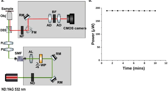
Figure 9. (a) Experimental setup that was used for imaging single molecules embedded in a thin polymer film sample. ND– neutral density filters, RM– reflecting mirror, WP- quarter waveplate. AL – aspherical lens, SMF

– single mode fiber, PL – pre-focusing lens, DBS- dichroic beam splitter, Obj- microscope objective, NF- notch filter, FM- flip mirror, AD- achromatic doublet, BF- bandpass filter. (b) Graph showing how stable the incident light was after coupling it through a single mode fiber, coupling efficiency was calculated to be 40 %.

(32)

18 Changing polarization state of incident light

The polarization state of the incident laser light is linear, however to ensure that the single molecules (assumed to be electric dipoles which are randomly orientated) were excited uniformly the polarization state of the incident light had to be changed. Since the electric dipole moments of the single molecules are randomly orientated on the cover slide after spin coating and excitation using linearly polarized light will not ensure uniform fluorescence emission from all the single molecules. Therefore, the use of circularly polarized light ensures that the electric field of light is always appropriately orientated with respect to the transition dipole moment in the single molecules which has the desired effect of uniform excitation of all dipoles and subsequently the uniform emission of the fluorescence.

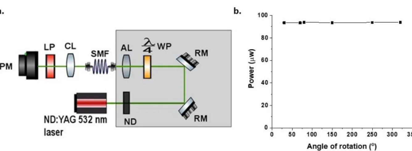
To achieve the aforementioned, the linearly polarized light was passed through a quarter waveplate positioned at 45ᵒ to its polarization axis to convert it to circularly polarized light. A quarter waveplate is made of birefringent material, that is a material with variations for index of refraction, because of these variations in the refractive index the orientation of the transmitted light is different and the phase between the two perpendicular polarization components of the transmitted light is shifted. To check if the linearly polarized light had changed to circularly polarized light, a linear polarizer was placed at one end of the fiber and a power meter also placed in front of the linear polarizer to measure the power intensity of the incident light as the linear polarizer was rotated. If the quarter waveplate was placed at an angle that ensures that linearly polarized light is changed to circularly polarized light, then the power intensity measured as the linear polarizer is rotated should remain constant since circularly polarized light has the same intensity in all directions (Figure 10).

(33)

19

Figure 10. (a) Experimental set-up to produce circularly polarized light through the insertion of a quarter waveplate. A linear polarizer was also introduced and was rotated in front of a power meter used to check the intensity of the polarized light. ND- neutral density filters, RM- reflecting mirror, WP- quarter waveplate, AL- aspherical lens, SMF- single mode fiber, CL- collimating lens, LP- linear polarizer, PM- power meter. (b) Graph shows the power intensity stability measured as the linear polarizer was rotated. From the graph it can be observed that the power intensity remained constant as the angle of rotation, thus the indicating that the polarization state of the excitation light was successfully changed to circular.

3.2 Sample preparation

In this section the preparation of single fluorescent molecules embedded in thin polymer films and deposited on glass cover slides will be discussed. Cleaning the glass cover slides also enhances the accuracy in the detection of the single molecules’ fluorescence, hence it is crucial that the cover slides are thoroughly and properly cleaned.

3.2.1 Cover slide cleaning

The glass slides are cleaned to remove any particulates that might fluoresce and affect the results. The cover slides (22x22 mm2_{) that were used for the samples were cleaned using a chemical protocol that}

contained the following reagents: 1. Ethanol 99,9% pure 2. H2O (Milli-Q filtered)

3. Potassium hydroxide pellets (KOH)

20 g of KOH (Sigma Aldrich) pellets were weighed and added to 60 ml of ethanol. The mixture was stirred vigorously to dissolve the KOH pellets. The KOH-filled beaker was placed in an ultrasonic bath and sonicated for 5 mins. Two beakers were filled with 60ml of Milli-Q water and sonicated for 5 mins and one

(34)

20

of the beakers is left the bath for a further 5 mins. The cover slides are placed in a custom-made Teflon rack and submerged in the KOH- filled beaker and sonicated for 5 mins. The Teflon rack is removed from the KOH solution and is rinsed by dipping it in the Milli-Q water until the water runs smoothly off the cover slides without beading.

3.2.2 Single molecule sample preparation

0.5 mg of perylene dye powder was dissolved in a volume of 4 mL of toluene and sonicated for 10 mins at 20 ᵒC to fully dissolve the powder, the concentration of the dye was calculated using equation (x) and found to be 0.50 mM. This sample was labelled as the stock sample concentration C

₀

and from the stock sample solution a volume of 5 μl was pipetted out and diluted with a volume of 4 ml of toluene in two stages to ensure that a very lowly concentrated solution. At each dilution stage, each sample solution was sonicated for 10 mins and at 20 ᵒC. The third sample solution labelled as sample concentration C

₃

with a concentration of 7.74 pM was calculated using equation (xi), were 100 μl from this sample solution was spin coated onto a glass cover slide and used for single molecule microscopy measurements.

C = m mrV (x) C0 = 0.5 mg 252.316 g/mol × 4 ml = 0.50 mM C3= C2 V2 V3 (xi) C3 = 61.93 nM × 0.5 μl 4 ml = 7.74 pM

3.2.3 Polymer sample preparation and thickness measurements

Prior to embedding dye molecules in the polymer, a generic procedure to create polymer thin films was developed and the thickness of the films was determined using UV-Vis absorption measurements together with accompanying calculations. In this work the dynamics of polystyrene with molecular weight Mw of

35 000 gmol⁻¹ (Sigma Aldrich) and poly (isobutyl methacrylate) with molecular weight Mw of 70 000 gmol⁻¹

(Sigma Aldrich) were investigated. To produce thin films, 92.7 mg of polystyrene beads and 115.8 mg of poly (isobutyl methacrylate) beads were weighed on a digital mass meter and then dissolved in 4 ml of toluene separately. Both polymer solutions were dissolved further into two solutions and sonicated for C- concentration of solution, m- mass of solute, mᵣ - molar mass of perylene dye and V – volume of solvent.

(35)

21

30 mins at 20 ᵒC. The concentration of the polymer solutions was calculated using equation (xii) and found to be 0.40wt% and 0.75wt% for polystyrene and poly (isobutyl methacrylate) respectively.

cwt% = weight of solute

weight of solvent× 100% (xii)

These polymer/solvent stock solutions were used to produce polymer thin films on the cover glass slides. Thin films were produced by dropping a predetermined concentration and volume of the polymer/stock solution on a rapidly rotating glass slide. This process is referred to as spin coating and it is well understood that the thickness of the film can be precisely controlled by choosing the appropriate spin speed. In order to determine the actual film thickness, the UV absorption of the polymer is used as a thickness measure. This is simple to understand as a thicker film would result in an increase in absorbance measured using the UV-VIS spectrophotometer. A volume of 100 μl of 0.4 wt% of polystyrene solution was spin coated onto a magnesium fluoride mirror at 640 rpm. Magnesium fluoride was chosen as it has a negligible absorbance at the desired absorption maximum of the polymers.Traditionally, using the Beer-Lambert Law the measured absorbance is equated to the molar absorptivity multiplied by the sample concentration and the optical path-length (here the thickness of the sample). However, the molar absorptivity for polymer films are not readily available and without knowledge thereof one cannot determine the thickness quantitatively. A convenient strategy to overcome this limitation, is to recognize that the absorption A must also be proportional not only to the thickness of the sample l but also to its density ρ (equation xiii).

A ∝ ρl (xiii)

The thickness of the spin coated polymer film is then determined using the densities of a liquid polymer solution and that of the solid spin coated polymer film. The method of thickness determination is given by the ratio of the absorbances for the liquid polymer Abs1 to that of the solid thin polymer Abs2 shown in equation (xiv).

Abs1 ∝ ρ1l1

Abs2 ∝ ρ2l2 (xiv)

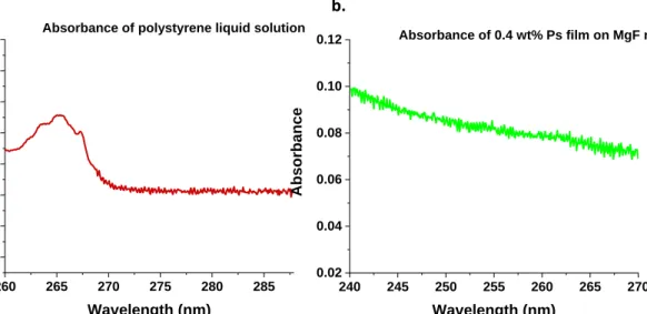
The absorbance of a known mass and volume of a polystyrene liquid was measured in a standard 1 cm UV-vis cuvette at a selected peak wavelength of 260 nm . The absorbance of the spin coated 0.4 wt% polystyrene film was measured at the selected wavelength,with the assumption that the density of the spin coated polystyrene is the same as that of a bulk polystyrene film (Figure 11). The thickness of the solid 0.4 wt% polymer film on the magnesium fluoride mirror was determined using equation (xiv), since the only unknown is the solid film thickness l2 and calculated as 941 nm.

(36)

22

Figure 11. The thickness of polystyrene films is determined using the ratio of absorbance of liquid polystyrene solution (a) and that of a solid polystyrene film spin-coated on a MgF slide (b), were the absorbance is proportional to the density of the material and its length/thickness. The absorbance of the liquid polystyrene liquid solution was measured to be 0.5 and that of the polystyrene film 0.1.

The thickness of the polymer sample can be varied by changing the spin speed for spin coating [33]. The thickness of the film is related to the spin speed through equation (xv).

h ∝ ω

−23

_(xv)

The films that were used in this work were spin coated at a spin speed of 2000 rpm and thus the thickness is < 900nm. From dye sample solution , 5 μl ,1 μl was pipetted out and mixed with 200 μl ,300 μl of the polystyrene and poly (isobutyl methacrylate) solutions respectively and sonicated for 30 mins at 20 ᵒC to thoroughly mix the two solutions. 100 μl from the mixed dye and polymer solution was spin coated onto a coverslide, the sample was heated up to 80 ᵒC under vacuum for 5 hrs so as to evaporate any residual solvent remaining and also to remove any stresses and strains on the polymer film due to the spin coating procedure. This relaxed polymer film sample was then used to carry out single molecule microscopy measurements.

3.3 Setup characteristics

In this section the designed optical system is characterized using the image calibration factor which is used for determining the distance between single molecules. The localization precision is also used for system characterization, it is used to describe the limit to which a fluorescing point object can be located. Long term microscope stage position stability conditions are discussed, and these influence the ability of a microscope to maintain the selected focal plane over extended periods of time. Lastly the design of a custom-made heating stage used for heating the polymer film samples is described.

h- thickness of sample and ω – spin speed.

260 265 270 275 280 285 -0.4 -0.2 0.0 0.2 0.4 0.6 0.8 Absorbance Wavelength (nm) 240 245 250 255 260 265 270 0.02 0.04 0.06 0.08 0.10 Absorbance Wavelength (nm)

(37)

23 3.3.1 Image calibration

Image calibration is used to be able to distinguish in real space the distance between two single molecules. A 10 µm calibration gridded slide was illuminated with a halogen lamp from the microscope objective and an image was captured using the CMOS camera. The image was then processed using ImageJ, a horizontal cross-sectional line cut-out was drawn across the image to get an intensity profile of the gridded slide (in red), the resulting cross-sectional intensity profile. The full width at half height along the intensity profile (indicated in Figure 12) was 270 pixels. These 270 pixels in real space is equal to 10 μm, thus giving us a convenient calibration factor. The relationship between real space dimensions and CMOS pixel dimension is:

μm: pix calibration factor = 10 μm

270 pix= 0.037μmpix

−1_{= 37 nmpix}−1

Figure 12.Image on the left shows the grayscale image of the calibration grid and on the right, the intensity profile resulting from cutting along a horizontal line drawn across the grid using ImageJ. 270 pixels counted on camera represents 10µm in real space dimensions of the grid imaged.

The calibration factor helps in finding the distance between single molecules for instance if two fluorescing point objects are 20 pixels from one another, then the distance in real space between the two fluorescent single point objects is 20 pixels * 37 nmpix⁻¹ = 740 nm.

3.3.2 Localization precision

The localization precision in single molecule resolved fluorescence microscopy is a measure which provides a simple yet intuitive way to determine the limit to which a fluorescing point object can be located. For single molecules, the localization precision is calculated as the standard deviation (σLP) of the loci xi_l (position of maximum intensity for the single molecule) over a number N of captured frames (expression xvi).

(38)

24

σ

_LP

= √

∑

(x

iI

− x

̅ )

I 2 N i=1

N − 1

(xvi)

Eleven individual fluorescent perylene dye molecules embedded in a thin polystyrene matrix were imaged over 100 frames and their loci found using Image J software, from which the localization precision was calculated in both X and Y directions using equation (xvi). The mean localization precision was calculated as 19.18 nm ± 10 nm and 19.45 nm ± 9 nm in X and Y respectively.

Figure13.Localization precision of single fluorescent perylene dye molecules embedded in polystyrene (circled in red) were imaged over 100 frames, camera exposure time of 500 ms and at a temperature of 17 ᵒC. The loci of the individual emitters were used to calculate the localization precision in both the X σ = 5 nm (bottom left)

and Y σ = 6 nm (bottom right) directions. The deviation in the localization precision is a result of the polymer chain nano-environment which is known to be complex as was studied by Tomczak et al [34].

N – number of frames