Applications in Spatial Cluster Analysis and
Bioinformatics
Dissertation
by
Martin Sch¨afer
Submitted to
the Faculty of Statistics
of the TU Dortmund University
in Partial Fulfillment of
the Requirements for the Degree of
Doktor der Naturwissenschaften
Prof. Dr. Katja Ickstadt
Prof. Dr. J¨org Rahnenf¨uhrer
In many statistical applications, one encounters populations that form homoge-nous subgroups regarding one or several characteristics. Across the subgroups, however, heterogeneity may often be found. Mixture distributions are a natural means to model data from such applications.
This PhD thesis is based on two projects that focus on such applications. In the first project, spatial nanoscale clusters formed by Ras proteins in the cell membrane are investigated. Such clusters play a crucial role in intracellular communication and are thus of interest in cancer research. In this case, the subgroups are clustered and non-clustered proteins.
In the second project, epigenomic data obtained from sequencing experi-ments are integrated with another genomic or epigenomic input, aiming, e.g., to detect genes that contribute to the development of cancer. Here, the sub-groups are defined by a) genes presenting congruent (epi)genomic aberrations in both considered variables, b) genes presenting incongruent aberrations, and c) genes lacking aberrations in at least one of the variables.
Employing a Bayesian framework, objects are classified in both projects by fitting finite univariate mixture distributions with a small fixed number of components to values from a score summarizing relevant information about the research question. Such mixture distributions have favorable characteristics in terms of interpretation and present little sensitivity to label switching in Markov Chain Monte Carlo analyses. Mixtures of gamma distributions are considered for Ras proteins, while mixtures of normal and exponential or gamma distribu-tions are a focus for the bioinformatic analysis. In the latter, classification is the primary goal, while in the Ras protein application, estimating key parameters of the spatial clustering is of more interest.
The results of both projects are presented in this thesis. For both applica-tions, the methods have been implemented in software and their performance is compared with competing approaches on experimental as well as on simulated
ter point process model called the double Mat´ern cluster process is developed and described in this thesis.
First of all, I wish to thank my advisor Katja Ickstadt for her guidance during my PhD time, in particular for giving me both freedom in many research problems and valuable advice whenever needed, but also for providing an always very comfortable working atmosphere in her research group.
Alan E. Gelfand supported my research on spatial Ras protein clusters through helpful discussions on concepts. I therefore would like to thank him for advice and for sharing his large statistical experience.
I would like to thank Peter Verveer and members of his former research group at the Max Planck Institute of Molecular Physiology in Dortmund for providing the problem regarding the research on Ras protein clusters, as well as for the fruitful collaboration in general. In particular, I want to thank Yvonne Radon for furnishing me with experimental Ras data and Thomas Klein for making my MATLAB code more efficient.
My research on spatial Ras protein clusters formed part of the project ‘Mod-eling spatial effects of cellular signals’ in the Research Training Group 1032/2 ‘Statistical Modeling’ funded by the Deutsche Forschungsgemeinschaft (DFG). I was granted a PhD scholarship for my research within this Research Training Group and would like to gratefully acknowledge this financial support.
I wish to thank Hans-Ulrich Klein, now Harvard Medical School/Brigham
and Women’s Hospital, Boston, and formerly University of M¨unster, M¨unster,
for our fruitful collaboration for years in the analysis of genomic and epigenomic
data, in which I feel we have complemented one another very well. I also
thank Martin Dugas, his former group leader at the University of M¨unster, for
supporting our work.
I thank my colleagues for numerous discussions on statistics. Representing many others, in particular I mention Jakob Wieczorek, with whom I shared an office at the Faculty of Statistics, TU Dortmund University, and Bernd Bischl, with whom I shared many coffees during conversations there in the last years.
I thank Holger Schwender, Philipp Berger, Julia Schiffner, Sabrina Herrmann,
Claudia K¨ollmann, Lars Koppers and Jenny Peplies for proofreading this thesis.
Further thanks go to Eva Brune and Brigitte Kupiec for administrative sup-port.
Equally important as work-related aspects, my friends have been providing support in many other ways. Thank you!
I am deeply grateful to Jutta and Thomas as I could not imagine better
parents . . . and they have made me what I am to a great extent. Thomas also
gave me the idea to study statistics by sharing his experience about this exciting profession with me.
Jenny has always been a wonderful big sister and friend, and I am glad to have her!
Finally, I thank Tamara for patience and emotional support during my PhD time... gracias mi vida... eres maravillosa y te amo!
1 Introduction and Motivation 1
2 Background 9
2.1 Genetic and Epigenetic Measurements . . . 9
2.2 Ras Proteins . . . 17
3 Mixtures and Clustering 23 3.1 Bayesian Mixtures . . . 23
3.1.1 Basic Definition . . . 23
3.1.2 Prior Distributions . . . 26
3.1.3 Identifiability and Label Switching . . . 33
3.2 Model Fitting . . . 35
3.2.1 The Expectation-Maximization (EM) Algorithm . . . 35
3.2.2 Markov Chain Monte Carlo Algorithms . . . 37
3.2.3 The Number of Components . . . 41
3.3 Cluster Analysis . . . 44
4 Spatial Modeling of Ras Protein Structures 50 4.1 Point Processes . . . 51
4.1.1 Properties of Spatial Point Processes . . . 52
4.1.2 Spatial Point Process Models . . . 55
4.1.3 Spatial Cluster Processes . . . 58
4.2 The double Mat´ern Cluster Process . . . 61
4.3 Data . . . 68
4.4 State-of-the-art Methods . . . 71
4.4.1 K-function Analysis . . . 71
4.4.2 DBSCAN . . . 73
4.4.3 Model-Based Clustering . . . 74
4.5 The GAMMICS Method . . . 77
4.5.1 Model . . . 77
4.5.2 Algorithmic Step to Estimate Cluster Sizes and Cluster Radii . . . 80
4.5.3 Sampling and Robustness Measures . . . 83
4.6 Monte-Carlo Tests for GAMMICS . . . 85
4.7 Results . . . 87
4.7.1 Simulated Data . . . 89
4.7.2 Experimental Data . . . 100
5 Integrative Analysis of Omics Data 106 5.1 Methodological Review . . . 107
5.2 Adaptation of the Externally Centered Correlation Coefficient . 118 5.3 Validation of ChIP-seq vs. ChIP-chip Techniques . . . 124
5.3.1 BCR-ABL Data Set . . . 125
5.3.2 Data Preprocessing . . . 127
5.3.3 Approach . . . 128
5.3.4 Results . . . 131
5.4 Integration of Histone Modification and Gene Transcription Data . . . 137
5.4.1 Data Sets . . . 137
5.4.2 Data Preprocessing . . . 139
5.4.3 Approach . . . 141
5.4.4 Results on CEBPA Knockout Data Set . . . 147
5.4.6 Results on ATRA/TCP Data Set . . . 159
5.4.7 Results on Simulated Data Set . . . 161
6 Summary and Discussion 163 A Additional Documentation and Results 178 A.1 Technological Background of Omics Measurements . . . 178
A.2 GAMMICS Method: Full Conditional Distributions . . . 185
A.3 GAMMICS Method: Sampling Scheme . . . 186
A.4 GAMMICS Method: Additional Results . . . 188
A.4.1 Trace Plots . . . 188
A.4.2 Posterior Histograms Across Clusters . . . 192
A.4.3 Posterior Histograms Across MCMC Iterations . . . 194
A.4.4 Results of Simulation Study in Detail . . . 198
A.5 BUGS Model: Full Conditional Distributions . . . 208
A.6 BUGS model: Additional Results . . . 210
A.7 Epigenomix Model: Model Details . . . 211
A.7.1 Full Conditional Distributions for Model (5.6) . . . 211
A.7.2 Full Conditional Distributions for Model (5.7) . . . 212
A.8 Epigenomix Model: Sampling Scheme . . . 213
A.8.1 Sampling Scheme for Model (5.6) . . . 213
A.8.2 Sampling Scheme for Model (5.7) . . . 214
A.9 Normalization Methods for ChIP-seq Data . . . 215
A.10 Epigenomix Model: Additional Results . . . 218
B Additional Theoretical Considerations 240 C Software 246 C.1 R Code for Point Process Simulations . . . 246
C.1.1 Documentation . . . 247
C.2 R Code for Monte Carlo Tests . . . 260
C.2.1 Documentation . . . 260
C.2.2 Code . . . 265
C.3 MATLAB Code for GAMMICS . . . 273
C.3.1 Main Code . . . 273
C.3.2 Auxiliary Functions . . . 288
C.3.3 Example Code . . . 294
C.4 WinBUGS Code . . . 300
C.5 R/Bioconductor Package Epigenomix . . . 302
List of Abbreviations 309
List of Figures 311
List of Tables 317
List of Algorithms 320
Introduction and Motivation
Karl Pearson, sometimes referred to as one of the founders of mathematical statistics, introduced the use of finite mixture distributions as early as 1894. In that year, he fitted a mixture of two univariate normal components to crab measurements based on moments (Pearson, 1894). However, probably only since the introduction of the Expectation-Maximization (EM) algorithm (Dempster
et al., 1977), which considerably simplified the fitting of mixture models via the maximum likelihood principle, are such models widely employed for statistical modeling. Their popularity is due to the fact that they arise naturally when a
randomly mixed population consisting ofK subgroups with relative group sizes
π1∗, . . . , πK∗ is to be analyzed. In this frequently occuring situation, inference
is to be done on a random variable Y that takes values in Y ⊆ Rd and is
homogenous within the subgroups, but heterogenous across them. This random
variableY describes a characteristic of interest, e.g., physical measurements such
as the ratio of forehead to body length in the case of the crab data analyzed by Karl Pearson, or a score summarizing genomic variation that is indicative
of the likelihood of a gene to contribute to cancer development. By nature, Y
has distinct probability distributions p(y|θT), where θ = (θ1, . . . ,θK) is the
(multidimensional) parameter and T is the indicator variable assuming one of
the group labels k = 1, . . . , K. The p(y|θT) might be arbitrary parametric
Figure 1.1: Densities of three mixtures consisting of two univariate normal
distributions each (Figure A: μ1 = −1, μ2 = 1, σ2
1 = 1.25, σ22 = 2.5, π∗1 = 0.8;
Figure B: μ1 =−2, μ2 = 2, σ2
1 = σ22 = 2, π∗1 = 0.5; Figure C: μ1 = −1.5, μ2 =
3, σ2
1 = 2, σ22 = 0.5, π∗1 = 0.7).
densities, but are usually chosen from the exponential family. Mostly, they are
assumed to arise from the same parametric family with onlyθT differing across
the groups. In case of p(y|θT) from different parametric families, the θT may
be of different dimensions.
An important question is whether the group indicator T can be recorded
or not in addition to Y (Fr¨uhwirth-Schnatter, 2006). If it can, the probability
of sampling from subgroup T is πT∗, and Y given T follows p(y|θT). The joint
density p(y, T) can then be written as
p(y, T) =p(T)·p(y|T) =πT∗ ·p(y|θT).
If, however, the group indicator T cannot be recorded in addition to Y, a finite
mixture distribution arises. In this typical situation, the marginal density p(y)
is given by
p(y|θ,π∗) =π1∗p(y|θ1) +. . .+πK∗ p(y|θK) (1.1)
with weight vector π∗ = (π∗1, . . . , π∗K).
In Figure 1.1, it is visualized how a mixture consisting of just two normal components leads to a considerable increase in flexibility compared to a single
normal density: it may present skewness, tails of different thickness or even multimodality.
There are several advantages of analyzing mixture models in a Bayesian framework, e.g., an increased capability to cope with small sample sizes and a smaller susceptibility to problematic likelihood shapes such as local maxima or
unboundedness (for a detailed discussion, see Fr¨uhwirth-Schnatter, 2006). In
addition, finite Bayesian mixture models have a straightforward generalization to an infinite number of mixture components, leading to nonparametric Bayesian analyses (Ferguson, 1973; Lo, 1984).
There are many situations and applications in which the group indicator T
cannot be recorded – i.e. in which a finite mixture distribution as in (1.1) arises – but the mixture distribution is not of primary interest. Instead, the focus lies on the level of each observation, in particular on the allocation of observations
to the mixture components (i.e. on the values ofT) and measures derived from
this allocation. Applications of this kind can be found, e.g., in cluster and classification analyses (throughout this thesis, the term classification will refer exclusively to supervised learning in the sense of discrimination). In this thesis, Bayesian methods employing mixture distributions are described and developed for applications which bear characteristics of both of these research tasks. These procedures perform classification in the sense of allocating objects to previously well-defined classes, but they are similar to clustering in the sense that they are unsupervised, i.e. no training data are available on which the allocation of objects could be learned. Furthermore, in the applications motivating the work presented in this thesis, there are, in principle, no covariates available which could be used to build a classification model. The objects for which a sample
of Y is observed in this thesis are proteins in a cell (Chapter 4) or genomic
locations (Chapter 5), i.e. points (or intervals) in either R2 or R. The most
usual case of a mixture of normal distributions is considered in Section 5.3. However, a greater focus lies on mixtures of gamma distributions (Section 4.4) and mixtures of normal and either exponential or gamma distributions (Section
5.4), i.e. on non-standard cases in which the probability distributions in the groups may come from different parametric families. Bayesian nonparametrics,
which consider an infinite number of components K ∈ N, are not a focus and
only discussed as a possible alternative.
In a project of the former Research Training Group 1032/2 ‘Statistical Mod-eling’ at the Faculty of Statistics of the TU Dortmund University, spatial pat-terns of Ras proteins on the plasma membrane were investigated in collaboration with the Max Planck Institute of Molecular Physiology, Dortmund. Essential
results of this project have been published in Sch¨aferet al.(2015). Ras proteins
are small and measure only about 2-3 nm in diameter. In the project, a special regard was given to their nanoclustering. Nanoclusters are deemed important in intracellular communication, and by consequence, in the coordination of cell regulation. They might thus play a role in the growth and division of cells as well as in tumor development. For this reason, they are a target of biomedical research. Only in recent years, specific implementations of fluorescence mi-croscopy have been developed that provide the spatial resolution necessary to analyze intact, living cells on the nanoscale. In particular, photo-activated lo-calization microscopy (PALM) and stochastic optical reconstruction microscopy
(STORM) (Betzig et al., 2006) now reach this resolution.
A key hypothesis in the research project is that nanoscale Ras clustering takes a characteristic form in cancerous cells. This might allow to identify tumors in tissues, and, more importantly, eventually provide a means to inhibit them. The central biological goal is to assess whether the clustering behavior of Ras proteins differs between distinct experimental conditions, such as healthy vs. tumor cells. A first step towards this goal pursued in this thesis is to quantify key parameters of the clustering behavior, in particular the proportion of proteins forming clusters, the mean cluster size and the mean cluster radius. Estimates of these parameters may be compared across different experimental conditions. In addition to point estimates, the clustering parameters’ distributions are also of interest, since they contain more information and enable comparisons on
a better fundament. In this respect, the setting differs from classical cluster analysis focusing on the cluster partition. Simultaneous inference for all three above mentioned key parameters is challenging due to identifiability problems resulting from dependencies between cluster size and cluster radius.
The results of this project are presented in Chapter 4 of this thesis. In particular, a new Bayesian approach called GAMMICS (GAMma Mixtures for Inference on Cluster Structures) is proposed that fits a mixture model to the squared distances between proteins and their second nearest neighbors. Infer-ence for all parameters of interest is possible in this framework by incorporating algorithmic aspects into the model. For validation, an extensive simulation
study is carried out. A point process model based on the Mat´ern cluster
pro-cess (Mat´ern, 1986) is developed for this purpose. This point process model, the
double Mat´ern cluster process, accounts both for only a proportion of points to
cluster and for clusters on two level. Specifically, in addition to clusters, points may form metaclusters potentially containing clusters as well as single points. The GAMMICS method is compared to the popular DBSCAN algorithm for
density-based clustering (Ester et al., 1996) and to a Bayesian framework for
model based clustering (Fritsch and Ickstadt, 2009). In addition, a comparison
is made with a combination of these two approaches (Argiento et al., 2013) as
well as to Ripley’s K-function and derivations (see, e.g., Kiskowskiet al., 2009).
Another application of finite dimensional mixture models is the integrative analysis of different data inputs from ’omics’, i.e. a variety of research fields in molecular biology, such as genomics, transcriptomics, epigenomics and pro-teomics. These scientific fields have gained huge importance in recent years due to technological advances facilitating their analysis. In the past, the suc-cess of high-throughput microarray technology has helped to use omics data to gain a better understanding of mechanisms underlying disease pathogenesis on a molecular basis, e.g., in cancer research. In recent years, the surge of analyses based on sequencing technologies has further propelled the availability of omics data and dramatically increased its resolution. Besides leading to a variety of
univariate research, this development has already brought about integrative, mostly paired, analyses of different omics data types. Aims of these analyses include, in particular, the combination of information as well as the validation of results and conclusions obtained from a single omics data type. A prominent example are joint analyses of copy number and gene transcription data including
genomic and transcriptomic observations (see, e.g., Ortiz-Estevez et al., 2011;
van Wieringen and van de Wiel, 2009; Sch¨afer et al., 2009).
Chapter 5 of this thesis is concerned with the integrative analysis of omics data, in particular epigenomic data. It is based on a project conducted in collaboration with the Institute of Medical Informatics at the University of
M¨unster, and essential results have been published in Sch¨afer et al. (2012) and
Klein et al.(2014). In epigenomics, one focus of interest is the analysis of the
influence which modified histones – proteins around which the DNA winds – might have on the activation or inhibition of gene transcription. Knowledge about this influence, in turn, might help to get a better understanding of the development of genetically caused diseases. In particular, histone modifications have been reported to be fundamental to stem cell differentiation as well as to the genesis of cancer (e.g., Baylin and Jones, 2011; Dawson and Kouzarides, 2012).
In cancer research, one goal is to find so-called ’driver’ genes or transcripts that contribute causally to cancer development through harmful mutations and a consequently altered behavior, as opposed to others that also present con-spicuous behavior in cancer cells, but do so only as a normal reaction to the distorted functioning of other genes (’passengers’). To identify such drivers and discriminate them from passengers, one strategy in epigenomics is to find ge-nomic regions in which histone modifications differ between two relevant biolog-ical conditions, e.g., between cancer and normal cells, or between cells bearing a mutation of an epigenetic regulator and wildtype cells. The main focus is usu-ally on detecting epigenetic modifications occurring together with a change in gene transcription, since in this case there is more evidence for a contribution to
the phenotype or to cancer development. Hence, in many studies, genome-wide mRNA and histone modification levels are measured from the same samples. Besides their potential causative role in cancer, genes showing differences in both histone modification and gene transcription data are important for iden-tifying putative therapeutic targets for epigenetic drugs.
In this thesis, integrative approaches are proposed to identify interesting genomic loci based on measures inspired by the externally centered correlation
coefficient (Sch¨afer et al., 2009), a correlation coefficient developed to assess
whether differences observed between two collectives are equally directed in two input variables. Besides the identification of drivers, this approach is employed to assess the congruence between different technologies employed to measure histone modifications. Correspondingly, the two input variables are either a hi-stone modification measured with two different technologies technologies (Sec-tion 5.3) or a histone modifica(Sec-tion measured in addi(Sec-tion to gene transcrip(Sec-tion (Section 5.4). First, a Bayesian mixture model with a fixed number of Gaus-sian mixtures is proposed to investigate such equally directed differences, and is applied to an experimental data set. Second, a more general Bayesian mixture model is developed that reduces the number of necessary components by mixing distributions of different types, improving interpretability. This mixture model is validated in applications to several experimental and simulated data sets. It is also compared to a naive approach based on separate analyses of both input variables.
In the mixture model for Ras proteins, two classes are contemplated (clus-tered vs. non-clus(clus-tered proteins), whereas in the omics project three classes are considered (genomic loci with observed differences between two collectives that are either equally or unequally directed in two data inputs, and genomic loci for which such differences cannot be observed in at least one input). In both projects, a standard mixture model is extended to satisfy needs posed by the re-spective scientific questions: in the Ras project, the model is complemented by an algorithmic post-processing step to carry out further, otherwise untractable
estimations of additional parameters, while in the omics project, classes may be represented by several mixture components and the type of distribution may vary across classes.
This thesis is organized as follows: in Chapter 2, biological and biotechnical background information is presented for the problems tackled in the two main projects, while Chapter 3 gives a theoretical overview on mixture models and a brief description on clustering methods. Chapter 4 is dedicated to the project on the spatial analysis of Ras proteins. Specifically, in Section 4.4, the simula-tion setup for validating the considered methods is described. Subsequently, the GAMMICS method and the considered competitors are described. The perfor-mance of these methods on the simulated and experimental data is reported in Section 4.7. The focus of Chapter 5 lies on the integrative omics project: Section 5.2 considers the adaptation of the externally centered correlation coefficient. Approaches for the integrated analysis of sequencing-based histone modification measurements and another omics input are described in Section 5.3 and Sec-tion 5.4 along with results, respectively. Finally, the results of the analyses are summarized and discussed in Chapter 6. In the Appendix, supplementary plots
and tables are displayed, MATLAB,Rand BUGS code for methods proposed in
this thesis are documented, and additional theoretical considerations omitted in the main text are given.
Background
In this chapter, first the biological background on genetic and epigenetic mea-surements is discussed, followed by a detailed description of the biology of Ras proteins. The order of these topics reflects the fact that proteins arise as a product of gene transcription. For a more detailed introduction to molecular genetics, see, e.g., Strachan and Read (1999).
2.1
Genetic and Epigenetic Measurements
All living organisms consist of basic units called cells. They contain
fundamen-tal elements of the respective organisms, such as the genomic information, and
are delimited by a plasma membrane. The genome of an organism has the role
of coding its structure and its functionality at the cellular level. It is stored
by means of the deoxyribonucleic acid (DNA), which in eucaryotes (organisms
whose cells contain a nucleus) mostly coils to form chromosomes. Humans, as
well as most animals, have a diploid set of chromosomes, i.e. every chromosome is available in two copies, where one copy comes from each parent. The number of chromosome pairs varies between species. Humans, e.g., have 23 and house mice (in Latin: mus musculus) 20 pairs of chromosomes in the nucleus of every
somatic cell. Somatic cells (from Greek ‘soma’= body) are all cells which are not germ cells or gametes (responsible for sexual reproduction) or stem cells.
Figure 2.1: Structural composition of the DNA. Its two spiral strands are long chains of nucleotide molecules, each nucleotide consisting of three elements: phosphate (P), the sugar (S) deoxyribose and one of the four bases adenine (A), cytosine (C), guanine (G), and thymine (T). Bases lying on opposed strands at the same position are connected via hydrogen bonds, where adenine always binds to thymine and cytosine always binds to guanine (key-lock-principle). Source: Schwender (2007).
The DNA has the form of a double helix, i.e. two intertwined spiral strands
con-sisting of long chains of nucleotides (see Figure 2.1). A nucleotide is a molecule
consisting of phosphate, the sugar deoxyribose and one of the four bases ade-nine (A), cytosine (C), guaade-nine (G), and thymine (T). Bases lying on opposite sides at the same DNA location are connected via hydrogen bonds, where ade-nine always binds to thymine and cytosine always binds to guaade-nine. Due to this key-lock-principle of the bases known as complementary base-pairing, it is sufficient to know the nucleotide sequence of just one of the two strands in order to possess the full coded information. The length of DNA fragments is usually measured in ‘base pairs’ (bp). Due to conventions regarding the naming of carbon atoms in the nucleotides on a chemical level, genomic loci are usually referred to relative to each other as ‘towards the 3 prime end’ (downstream, short: 3’ end) or ‘towards the 5 prime end’ (upstream, short: 5’ end) on one of the DNA strands.
Besides the DNA, the chromosomes also contain proteins, most of which are
histones around which the DNA winds. The formation of this DNA-protein
the DNA, guaranteeing that it fits into the cellular nucleus.
Structurally, the information stored in the DNA consists of genes, small
sections each containing the blueprint for one or more proteins.
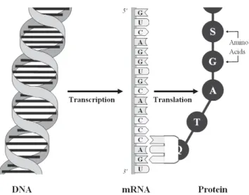
Proteins are fundamental components of cells responsible for virtually all body functions of living organisms. The central dogma of molecular biology (see Figure 2.2) describes how the information coded in genes is used to form
proteins: first, the DNA is transcribed intomessenger ribonucleid acid (mRNA)
by means of the enzyme RNA polymerase. The mRNA is similar to the DNA,
but consists only of one strand and contains a different sugar molecule (ribose instead of deoxyribose) as well as a different base (uracil instead of thymine).
After thistranscription, the mRNA leaves the cell nucleus. The mRNA product
of a gene is called transcript. Duringtranslation, sequences of three consecutive
nucleotides of the mRNA are translated into one of 22 amino acids forming a
chain that coils into a protein.
The amount of specific mRNA detected for a specific organism and DNA
locus is referred to as(gene) transcription level. The termgene expression (GE)
is often used synonymously to gene transcription, but sometimes refers to the entire process that forms a protein using the information coded in the DNA sequence of a gene. To avoid misunderstandings, the term gene transcription is generally used in this thesis (except for the commonly used term ’gene expression microarray’). The position at which the transcription begins for a specific gene
is called its transcriptional start site (TSS).
Near the TSS of each gene, there exists a DNA region called promoter that
helps to direct the RNA polymerase to the correct position in order to begin transcription of this gene. To do this, it interacts with DNA binding proteins
called transcription factors. If a gene codes for more than one protein, there
will consequently be several promoters and one speaks of alternative promoter
usage.
Structurally, genes can be viewed as a sequence of introns and exons.
Figure 2.2: The central dogma of molecular biology explains how proteins are formed based on the information coded in the DNA: The DNA is first tran-scribed into single-stranded messenger ribonucleid acid (mRNA) by means of the enzyme RNA polymerase. Subsequently, sequences of three consecutive nu-cleotides of the mRNA are translated into one of 22 amino acids, forming a chain that coils into a protein. Source: Schwender (2007).
into proteins, they are removed during a process called splicing. The remaining
DNA parts, the information-bearing exons (short for expressed regions), even-tually do code for proteins. However, for most genes the delimitations between introns and exons are defined only during splicing, resulting in several different
proteins generated from the same gene. This is called alternative splicing and,
according to estimates, affects approximately 60% of genes in humans (Chen, 2011). To take this into account, transcripts will be considered as elementary units instead of genes in Section 5.4 of this thesis.
The importance of genomic analyses in cancer research is owed to the fact that the DNA can vary between individuals of the same species. Even though most DNA is identical throughout a species, existing genetic variation may lead to different proteins, and hence to different risks for diseases such as cancer.
Genetic variation may arise in two different ways. One the one hand, genes
from both parents are regularly rearranged to form a new genome in
recombina-tion during reproduction. One the other hand, mutations may occur, resulting
muta-Figure 2.3: Possible chromosome mutations in humans. Two chromosomes are involved in insertions and translocations, while only one chromosome is involved in the other mutations. Source: Wikipedia (2014a), slightly modified.
tions are an integral part of evolution just as recombination, in many cases they lead to harmful rather than beneficial alterations of the genome and for this reason are frequently involved in the development of (genetic) diseases. When they occur in germline cells, they may be passed on to the next generation. If they occur in somatic cells, however, they only affect the organism in which they occur. In the context of investigating genetic causes of malign tumors, mostly somatic cells affected by cancer are examined. The possible occurrences of a gene, or, more general, of a specific sequence of nucelotides on the DNA,
are called alleles.
The number of copies of such an allele in the genome is generally referred to asDNA copy number or justcopy number (CN). In case of a diploid chromosome set, each of the two copies of the chromosome to which a specific DNA sequence belongs typically carries an identical copy of the sequence. This corresponds to a copy number of two, although exceptions exist, e.g., in case of the X-and Y-chromosome in males. Since the copy number refers to specific alleles, measurements of the copy number always refer to a reference genome, usually
Figure 2.4: Chromatin organization. Euchromatin (loose or open chromatin) structure is permissible for transcription and corresponds to histone acetyla-tion. Heterochromatin (tight or closed chromatin) structure is inhibitive for transcription and corresponds to histone methylation. Source: Sha and Boyer (2009).
the wild type, i.e. the most typical or frequent allele.
Mutations may affect DNA regions of very different sizes, from a single base to whole parts of chromosomes, and lead to structural alterations in these regions.
If a new DNA sequence variation becomes increasingly common in the ge-nomic pool, i.e. when the most infrequent allele in a DNA sequence reaches a frequency of 1% throughout a population, it is called a polymorphism. When the variation affects only a single nucleotide, i.e. only a single base is altered,
deleted, or added, it is referred to as a single nucleotide polymorphism (SNP).
Mutations of whole parts of a chromosome are caused by larger deletions, duplications, inversions, insertions, and translocations (see Figure 2.3) and may have a strong impact depending on their position. Translocations may be writ-ten in short in the form t(1;2) (denoting a translocation between chromosome 1 and chromosome 2).
gen-eration of proteins. These are usually referred to as epigenetic influences. One of these epigenetic influences is the modification of histones that may have ei-ther a repressive or an activating effect on gene transcription. On a chemical
level, methylation of histones generally results in a dense chromatin structure,
inhibiting gene transcription, whereas acetylation of histones leads to a loose
chromatin structure that activates gene transcription (see Figure 2.4). Inves-tigating the levels of methylation and acetylation may, thus, shed light on the extent to which gene transcription is being influenced epigenetically. Histone modifications are fundamental to stem cell differentiation as well as to the gene-sis of cancer (Baylin and Jones, 2011; Dawson and Kouzarides, 2012). Analyzing their functionality may, therefore, help to understand the cause of genetic dis-eases.
A central step in the measurement of omics data such as DNA copy num-ber, gene transcription and histone modifications is the quantification of DNA, mRNA, or DNA bound to histones, respectively. This implies the identification of the DNA fragments. For this procedure, inherent to analyses of all three men-tioned omics data types, several technologies have been proposed and constantly advanced regarding their throughput and resolution. The DNA fragments may be charged with fluorescent dye and hybridized to a microarray containing mil-lions of small fixed DNA sequences, on which the relative amount of hybridized DNA may be measured with a scanner. Alternatively, the DNA fragments may be sequenced directly using next-generation sequencing technologies and compared to a reference genome. Sequencing technologies provide maximum resolution and sensitivity without restriction to a fixed number of probes. Both microarrays and sequencing methods are described in more detail in the Ap-pendix A.1.
The measurement of histone modifications requires an additional pre-step, since not only amounts of DNA or mRNA, but interactions between DNA and proteins need to be measured. The standard method to approach such
bi-10,220,000 10,225,000 10,230,000
ChIP–seq input DNA ChIP–chip
ChIP–seq
NPC1 CG5708 CG5694
Pros35 CG4908 eEF1
Figure 2.5: Example profiles produced by chromatin immunoprecipitation fol-lowed by sequencing (ChIP–seq tag density; red) or microarray analysis
(un-logged ChIP–chip intensity ratio; blue). Shown are binding profiles of the
chromodomain protein Chromator in a Drosophila melanogaster cell line. The ChIP–seq profile reveals Chromator binding positions with higher spatial res-olution and sensitivity. The ChIP–seq input DNA (control experiment) tag density is shown in grey for comparison. Source: Park (2009).
ologic method for investigating bindings between DNA and proteins such as modified histones. In ChIP, DNA bound to histone proteins is sheared into small fragments in this context. Then, modified histones with DNA fragments wound around them are immunoprecipitated (i.e. isolated) by means of an an-tibody specific to the histones of interest. Afterwards, the genetic material is separated from the histones and quantified (Huss, 2010).
As an example, in Figure 2.5 ChIP binding profiles of the so-called Chroma-tor protein are compared resulting from analyses based on microarray (ChIP-chip; Mockler and Ecker, 2005) and sequencing technology (ChIP-seq; Park, 2009; Furey, 2012). This figure shows that the ChIP–seq profile has a higher spatial resolution and sensitivity, and the identified peaks – indicative of a sig-nal clearly distinguishable from noise – are sharper and narrower. A ChIP–seq control profile is also visualized which unsurprisingly does not exhibit any peaks.
The genomic locations obtained by sequencing technologies (ChIP-seq, RNA-seq, or other applications) result in count data as raw values when analyses are performed on a gene-wise level. Thus, a distinct preprocessing is required than for microarray experiments which render continuous raw values.
Microarray measurements have to be normalized to remove unwanted ef-fects like noise and artifacts in the signal. The specific normalization approach adopted in this thesis is discussed in Sections 5.3.2 and 5.4.2.
In sequencing experiments, the absolute number of DNA fragments found for
a specific genomic location (also called read count) depends on the sequencing
depth or coverage level, i.e. the number of times a genome is sequenced. The sequencing depth is arbitrarily chosen by the analyst according to a tradeoff: a higher sequencing depth leads to a higher sensitivity, but also to higher costs. To avoid an influence of the sequencing depth on the results of an experiment, either the absolute number of reads has to be adjusted for different sequencing depths across data sets by a normalization procedure, or a quantification other than the absolute number of reads has to be chosen. Specific methods employed in this thesis are discussed in Section A.9 of the Appendix as well as in Sections 5.3.2 and 5.4.2. Normalization approaches are often referred to as methods for the estimation of transcript abundance.
Specific methods for alignment of sequences and normalization are not dis-cussed in this thesis.
2.2
Ras Proteins
In Chapter 4, the spatial alignment of certain proteins on the plasma membrane of cells is of interest due to their role in intracellular communication. Cellular signal transduction plays an important role in cell regulation, i.e. in processes intended to maintain a balanced, healthy cell condition. Among other issues, this involves the regulation of the growth of a cell and its replication rate, both investigated in cancer research since tumors are a product of uncontrolled
growth and replication.
The communication between cells takes place by means of receptors, i.e.
specific proteins located on the cell surface or beneath it that bind chemical signals. Signals reaching the cell from outside through the receptors may lead to a variety of events within the cell, eventually activating mechanisms changing
its behavior in acellular responseto the signal. The cellular responses depend on
chemical and physical properties of the cells as well as on spatial inhomogeneities in the distribution of involved signaling proteins. Specifically, it is assumed that the spatial patterns of such proteins on the plasma membrane have an influence on their signaling behavior, and protein clusters occurring at a sub-micrometer scale are believed to be of relevance. However, it is still largely unknown how these clusters arise and what specific function they have in the
signal transduction (Jacobson et al., 2007).
The signaling chain of the epidermal growth factor (EGFR) on the plasma membrane, fulfilling an obvious role in cell regulation through its influence on cell growth, is regarded as an emblematic case of such protein clustering (Citri and Yarden, 2006). In particular, this signaling chain includes ErbB-1, the receptor of the epidermal growth factor, and subsequent steps belonging to
the regulatory circuit of the protein GTPase Ras. Both of these molecules
have key functions in signal transduction involved in processes related to cell development and growth. Such processes include maintaining the integrity of the cellular skeleton, cell differentiation, proliferation, and the controlled cell death. Thus, these molecules can play a major role in the development of tumors and are therefore a target for biomedical research. Both proteins also
do partly cluster on a nanometer scale (Hancock, 2006; Saffarian et al., 2007).
The work in this thesis focuses on the spatial clustering of Ras proteins, 2-3
nm in diameter, which have been given special research attention (Henis et al.,
2009; Prior and Hancock, 2012). Their name reflects their first discovery in the context of the investigation of rat sarcomas (sarcomas are malign tumors originating in connective tissues).
Figure 2.6: Signal transduction via Ras proteins: Signal molecules bind to (and activate) receptor tyrosine kinases (RTK), enzyme-coupled cell-surface recep-tors. An adaptor protein docks on a phosphotyrosine (P) on the activated receptor and recruits a Ras-activating protein that causes Ras to exchange its bound guanosine diphosphate (GDP) for guanosine triphosphate (GTP). The activated Ras protein can now stimulate several downstream signaling pathways.
Source: Alberts et al. (2010).
The Ras protein family has various members differing with respect to their chemical composition, in particular concerning the part anchoring them to the membrane. Two prominent examples are H-Ras and K-Ras.
Alongside many other proteins involved in propagating arriving signals fur-ther into the cell, Ras proteins are guanosine nucleotide-binding proteins, some-times referred to as binary molecular switches due to their two possible states. On the chemical level, such proteins may either bind to guanosine triphosphate (GTP) or guanosine diphosphate (GDP). Binding to GTP results in an active state, while binding to GDP leads to inactivity. In the literature, proportions of 30-45% of Ras proteins have been reported to form highly dynamic, short-lived nanoclusters having an average radius of 6-16 nm and an average cluster size of
6-7 proteins (Plowman et al., 2005; Tian et al., 2007; Kiskowski et al., 2009).
However, the methodology in these publications may be partly questioned from a statistical point of view, as will be discussed in Section 4.4.1. The clusters are formed by Ras during its inactive state and are assumed to be stabilized during
the active GTP-bound state. This results in the formation of signaling plat-forms possessing characteristics beneficial for the transmission of signals into
the cell (Tian et al., 2007; Rotblat et al., 2010). This process, symbolized in
Figure 2.6, eventually influences gene transcription involved in cell prolifera-tion and other cancer-related regulaprolifera-tions via a subsequent protein cascade. It has been demonstrated that inhibition of Ras clustering severely affects signal
transduction (Plowman et al., 2005). Moreover, Ras proteins deregulated as a
consequence of mutations have been found in cancers (Fern´andez-Medarde and
Santos, 2011; McCubrey et al., 2012).
The direct visualization of small clusters formed by signaling proteins such as Ras, in the order of less than 10 nm, has been a challenge until recently. Electron microscopy has traditionally been used to visualize the distribution of
Ras proteins (Plowman et al., 2005; Hancock, 2006), but it requires
destruc-tive preparation steps for the cellular material that can considerably affect the spatial patterns of interest. Fluorescence microscopy is a newer, alternative technology allowing to examine intact, living cells. However, it has to be com-bined with special methodologies to reach the necessary resolution. Indirect methods such as fluorescence resonance energy transfer (FRET microscopy) or fluorescence correlation spectroscopy (FCS) have been tested for this task, but these procedures are based on many physical assumptions and are not able to visualize the spatial protein distribution directly. Most recently, the develop-ment of photoactivated localization microscopy (PALM) and stochastic optical reconstruction microscopy (STORM) has made it possible to visualize single
molecules at an increased spatial resolution of roughly 20 nm (Betzig et al.,
2006).
In this thesis, a focus lies on the analysis of data generated with PALM in a setup briefly described in the following. Fluorescence microscopy in general is based on the excitation of fluorescent probes and the subsequent measurement of emitted light. In PALM, appropriate photoactivatable fluorophores such as paGFP, pamCherry, or mEos are genetically fused to the proteins to accomplish
Figure 2.7: Schematic overview of a fluorescence microscopy system. Light emanating from a light source such as a laser is directed at the cell specimen on the glass slide of a microscope by means of a mirror. The photons are absorbed by the specimen and then re-emitted by fluorophores fused genetically to the proteins of interest. An ocular or a digital camera connected to the microscope may then capture the light emitted by a single protein as a blob that covers a surface much bigger than the protein itself. Source: Wikipedia (2014b).
this. A laser dispenses light directed at the cell specimen on the glass slide of a microscope. The photons are absorbed and then re-emitted by the fluorophores, producing light that covers a surface much bigger than the proteins themselves. When instead of an ocular, a digital camera is connected to the microscope, this light can later be seen on resulting greyscale pixel images as blobs indicating the presence of a protein. The images analyzed here have a resolution of 512x512 pixels, where each pixel has a side length of 107 nm. Figure 2.7 shows the prin-cipal setup of a comprehensive fluorescence microscopy system in a schematic way.
The research effort presented in this thesis focuses on cells with an expression level above normal typical for cancer cells. In the experimental setup, cancer cells are mimicked by artificially overexpressed Ras, tagging it to a fluorescent protein. Due to the high expression level, not all proteins can be visualized and
detected as single molecules simultaneously because the corresponding blobs would overlap and render a completely white image. Thus, only a subset of
molecules are activated by UV light at a time (Hess et al., 2006), avoiding too
much overlap between the light blobs. After a reasonable time during which pictures are created every 100 milliseconds, it can be expected that the recorded blobs represent a vast majority of Ras proteins in the cell. The time necessary to record all proteins cannot be determined with certainty. Blobs may persist during several time frames recorded by the camera before they disappear. In some cases, proteins may be reactivated later (‘blinking’).
In an effort to limit sources of noise, the total internal reflection fluorescence technique (TIRF, Toomre and Manstein, 2001) is employed in combination with PALM. This ensures that only fluorophores in the basal membrane (up to 100-300 nm below the cell surface) are activated, while the fluorophores located deeper inside the cell, of no interest for the cluster phenomenons under investi-gation, are ignored.
Mixtures and Clustering
This chapter starts with an introduction to the theory of finite Bayesian mix-tures in Section 3.1. Subsequently, Section 3.2 contains brief descriptions of the principal techniques for fitting mixture models, i.e. the Expectation-Minimization (EM) algorithm and Markov Chain Monte Carlo (MCMC) algorithms. Parts of these first two sections follow roughly Section 2.1 in Fritsch (2010). Finally, in Section 3.3, methods for cluster analysis are briefly reviewed with an emphasis on model-based clustering.
3.1
Bayesian Mixtures
3.1.1
Basic Definition
As discussed in the introduction, a finite mixture distribution arises for a random
variable Y assuming values in Y ⊆ Rd when its marginal density p(y) is given
as a weighted sum over probability densities p(y|θk), i.e. as
p(y|θ,π∗) =
K k=1
πk∗p(y|θk) (3.1)
where it isπk∗ ≥0 for k = 1, . . . , K, and Kk=1π∗k= 1, with parameter vector
θ = (θ1, . . . , θK) and weight vector π∗ = (π1∗, . . . , πK∗ ). For the discussion in
this section, K may also be infinite. Existence of densities with respect to the Lebesgue measure will henceforth be assumed.
There are many applications, e.g., cluster and classification analyses, in which the allocation of observations to the mixture components and measures derived from this allocation are of interest rather than the mixture distribu-tion itself. In these cases, the model (3.1) can be reformulated to account
for these research focuses by introducing an extra variable T that represents
the allocations to the mixture components. Thus, πk∗ = P(T = k|π∗) and
p(y|θk) =p(y|T =k,θ) so that (3.1) becomes p(y|θ,π∗) = K k=1 P(T =k|π∗)p(y|T =k,θ).
In classification analysis, T = k represents a classification of an object to
class/componentk, while in cluster analysis, it stands for an allocation to cluster
k.
A mixture model estimates π∗ and θ as basis for classifying objects. In a
situation in which they are known, the conditional distribution of T|y can be
obtained by Bayes’ theorem, i.e. by
p(T = ˜k|y,θ,π∗) = π ∗ ˜ kp(y|θk˜) K k=1πk∗p(y|θk) , (3.2)
and an object is classified by assigning it to the class ˜k that maximizes (3.2).
Considering realizations y = (y1, . . . , yn) of independent random variables
Y1, . . . , Yn for which the general mixture model (3.1) is assumed, the likelihood
function can be written as
p(y|θ,π∗) = n i=1 p(yi|θ,π∗) = n i=1 K k=1 πk∗p(yi|θk) . (3.3)
If, again, the focus is on the individual allocations T = (T1, . . . , Tn), (3.3) can
I(Ti =k), leading to p(y|T,θ) = n i=1 K k=1 I(Ti =k)p(yi|θk) = n i=1 K k=1 p(yi|θk)I(Ti=k) .
In the simplest case of K = 2, considered in Chapter 4, π∗ = (π∗,1−π∗). In
this case, Ti ∼Bernoulli(π∗) is a reasonable assumption, i.e.
p(T|π∗) = n i=1 (I(Ti = 1)π∗+I(Ti = 2)(1−π∗)) = n i=1 π∗I(Ti=1)·(1−π∗)I(Ti=2) . (3.4)
For notational consistence, let the possible realizations of the Ti be 1 and 2
in this section, instead of the common values 0 and 1. For a general K > 2,
it is assumed that Ti ∼ Categorical(π1∗, . . . , πK∗), i.e. the allocation variable Ti
follows a categorical distribution,
p(T|π∗) = n i=1 K k=1 I(Ti =k)πk∗ = n i=1 K k=1 πk∗I(Ti=k) = K k=1 πk∗ni=1I(Ti=k). (3.5)
The categorical distribution, thus, is a generalization of the Bernoulli distri-bution for a categorical variable with more than two possible outcomes. The likelihood (3.3) in this notation is obtained as
p(y|T,θ) =
T∈{1,...,K}n
p(y|T,θ)·p(T|π∗).
For notational convenience, the abbreviation nk :=
n
i=1I(Ti = k) will be
used in the remainder of this thesis for the number of observations allocated to
3.1.2
Prior Distributions
In a Bayesian framework, it is necessary to specify prior distributions for the
model parameters. The parameters θ and π∗ are usually assumed to be
inde-pendent a priori so that
p(θ,π∗) =p(θ)p(π∗).
The specification of the mixture prior mixture p(π∗) will be discussed with
particular attention. In the simplest case of K = 2, whereπ∗ = (π∗,1−π∗), a
Beta prior with parameters aπ∗, bπ∗ >0 is assumed for π∗1 with density
p(π∗) = Γ(aπ∗)Γ(bπ∗)
Γ(aπ∗+bπ∗)
π∗aπ∗−1(1−π∗)bπ∗−1 ∝π∗aπ∗−1(1−π∗)bπ∗−1·I(π∗ ∈[0,1]).
The posterior distribution with density
p(π∗|T)∝π∗aπ∗+n1−1(1−π∗)bπ∗+n2−1
is a Beta(aπ∗ +n1, bπ∗ +n2) distribution, i.e. it has the same functional form
as the prior. The Beta distribution is thus by definition the natural conjugate
distribution for the Bernoulli distribution of Ti in (3.4). When K > 2, the
standard prior for π∗ = (π1∗, . . . , π∗K−1,1−Kk−1π∗k) is a Dirichlet distribution
with parameter α = (α1, . . . , αK), αk >0 for k = 1, . . . , K. This distribution
has the density
p(π∗) = K k=1 π∗kαk−1· Γ( K k=1αk) K k=1Γ(αk) ∝ K k=1 πk∗αk−1·I(π∗ k ∈[0,1])
and will be denoted by Dirichlet(α). Analogously to the caseK = 2, the
Dirich-let distribution is the natural conjugate prior for the categorical distribution of
T in (3.5), since the posterior
p(π∗|T)∝p(T|π∗)p(π∗)∝
K k=1
is a Dirichlet(α1+n1, . . . , αK+nK).
As reflected by these relationships, the Dirichlet distribution is the multivari-ate generalization of the Beta distribution. The natural conjugacy (henceforth: conjugacy) of the Beta and Dirichlet distributions, respectively, is a principal motivation for employing them, since choosing conjugate prior distributions in Bayesian statistics always has advantages when fitting the model. Conjugate prior distributions have computational benefits: in simple models they often al-low an analytical computation of the posterior distribution, while in more com-plex models, they facilitate the use of the Gibbs sampler in MCMC approaches (for details, see Section 3.2.2). Conjugate prior distributions also often help to interpret results and have the nice property of being interpretable as additional
data (Gelman et al., 2013).
There exist several extensions and generalizations of the Dirichlet distribu-tion. Important examples are the generalized Dirichlet distribution (Ishwaran and James, 2001) or the two-parameter Poisson-Dirichlet distribution (Pitman and Yor, 1997).
The numerous priors for infinite mixture models discussed in the field of nonparametric Bayesian statistics can, at least in their great majority, also be viewed as extensions or generalizations of the Dirichlet distribution. The oldest and most important one is the Dirichlet process (Ferguson, 1973) that induces Dirichlet distributions when data are grouped into any finite measurable partition, exploiting the conjugacy of the Multinomial-Dirichlet model for this setting. The Dirichlet process mixture (DPM) model introduced by Lo (1984)
(see also MacEachern and M¨uller, 1998) is one of the most frequently employed
Bayesian mixture models.
For the Dirichlet process in turn, many modifications and generalizations have been developed. For example, several hierarchical extensions have been in-troduced. While they facilitate to appropriately borrow information across data originating from distinct sources such as different study centers, they also help
of covariates (Dunson, 2010). These extensions, in particular, include mixtures
of independent Dirichlet processes (M¨uller et al., 2004), dependent Dirichlet
processes (McEachern, 1999), hierarchical Dirichlet processes (Teh et al., 2006),
and nested Dirichlet processes (Rodriguez, 2008).
Recent developments include latent stick-breaking processes that, in contrast to other nonparametric models, facilitate anisotropic and nonstationary models
(Rodriguez et al., 2010). Another recent proposal are probit stick-breaking
processes, in which the characteristic beta distribution in the stick-breaking construction, see the definition in (3.8), is replaced by probit transformations of normal random variables (Rodriguez and Dunson, 2011).
Overviews on the rapidly evolving field of Bayesian nonparametrics are given
in Ghosh and Ramamoorthi (2003) and Hjort et al. (2010). A comprehensive
theoretical overview of classes of nonparametric priors providing more flexibility
than the Dirichlet process is given, in particular, by Lijoi and Pr¨unster (2010).
A connection between finite and infinite mixture models exists in truncated versions of infinite mixture models such as the truncated Dirichlet process, in
which an upper bound is fixed for the number of components K,
approximat-ing the infinite by a finite mixture model (see Ishwaran and Zarepour, 2000; Ishwaran and James, 2001). When a high number of components is used, the difference to an infinite mixture becomes negligible, while the dimensionality of the model can be kept fixed, leading to computational benefits (cf. Section 3.2.3).
A general class of both finite and infinite mixture priors is the class of Ongaro-Cattaneo random measures (Ongaro and Cattaneo, 2004):
Definition 3.1 (Ongaro-Cattaneo probability measures).
A random discrete probability measure P is called Ongaro-Cattaneo probability measure if it can be written as
P = K k=1 πk∗δζ∗∗ k, (3.7)
Priors with K <∞ ak bk Note
Dirichlet distribution αk Kk∗=k+1ak∗ k= 1, . . . , K−1, setVK = 1
Finite-dimensional Dirichlet α∗/K Kk∗=k+1ak∗ k= 1, . . . , K−1, setVK = 1
Trunc. Dirichlet(α0) process 1 α0 set πK∗ = 1−Kk=1−1πk∗
Priors with K =∞
Dirichlet(α0) process 1 α0
Pitman-Yor(a,b) process 1−a b+ka a∈[0,1),b >−a
Table 3.1: Sampling of known priors via stick-breaking construction. For
the Dirichlet distribution, the finite dimensional Dirichlet prior, the truncated Dirichlet process, the Dirichlet process and the Pitman-Yor process,
correspond-ing choices for a= (a1, . . . , aK) andb = (b1, . . . , bK) are listed when sampling
the proportions Vk∼Beta(ak, bk) independently. It is ak, bk, α∗, α0 >0.
where K, πk∗, and δζ∗∗
k are random variables with the following properties: K is
a positive integer or ∞. The weights π1∗, . . . , πK∗ , conditional on K, have an arbitrary distribution on the (K−1)-dimensional simplex
SM = π∗ ∈RK :K k=1πk∗ = 1, πk∗ ≥0, k= 1, . . . , K . Theδζ∗∗
k are an i.i.d. sample of a nonatomic distributionP0onΞ
∗ (i.e.P
0({ζk}∗ ) =
0 ∀ζk∗ ∈Ξ∗), independent of πk∗, k= 1, . . . , K, and K.
An important subclass of Ongaro-Cattaneo priors are stick-breaking priors. Stick-breaking priors have the Ongaro-Cattaneo form (3.7), but assume that
K is fixed (with the possibility of K = ∞) and that the weights are sampled
according to π1∗ =V1 and π∗k=Vk k−1 k∗=1 (1−Vk∗), (3.8)
where Vk are independent Beta(ak, bk) random variables, k = 1, . . . , K, and
ak, bk >0. In general, it is not guaranteed that
K
k=1πk∗ = 1. However, it can
be shown that assuming K = ∞ and ∞k=1log(1 +ak/bk) = ∞ ensures that
K
k=1πk∗ = 1. If K <∞, it is sufficient to set VK = 1, leading to a generalized
3.1, important stick-breaking priors are listed with their corresponding choices
forakand bk. All of the priors that are explicitly mentioned in this section may
be sampled by a stick-breaking construction.
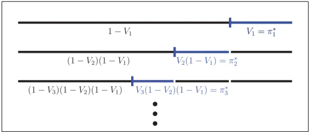
The term stick-breaking construction is owed to the fact that the sampling may be seen as a process in which pieces are consecutively broken off a stick of
length 1, see Figure 3.1. The Vk correspond to the proportion of the remaining
stick that is broken off. Wong (1998) discusses sampling from the generalized Dirichlet distribution and the Dirichlet distribution in particular via a stick-breaking construction, independently of their employment in mixture models. Ishwaran and James (2001) describe the sampling of stick-breaking priors in a general framework.
To date, the Dirichlet distribution remains a very frequently used mixture prior in finite mixture models due to its simplicity and its conjugacy properties. Unless specific reasons suggest otherwise, mostly an exchangeable symmetric
Dirichlet prior with αk ≡ α0, k = 1, . . . , K, is chosen that does not favor
any particular class. In this case, α0 is referred to as concentration parameter
(the same term and notation is used in the context of the Dirichlet process). A
widely used prior is the uniform Dirichlet prior withα0 = 1. However, Ishwaran
and Zarepour (2002a) discuss in the context of mixtures of normal distributions that there exist consistency problems with this prior. In particular, they show
that this prior is inconsistent when n/K → 0, i.e. when K gets too large in
comparison to n. To solve this issue, they recommend to re-parameterize the
symmetric Dirichlet prior such that α0 = α∗/K for an α∗ > 0 and show that
this prior is strongly consistent for the density and weakly consistent for the un-known mixture distribution. Moreover, Ishwaran and Zarepour (2002b) show
that it approximates the Dirichlet process for increasing K and that for a fixed
value of ζ∗ = (ζ1∗, . . . , ζK∗) it is already a Dirichlet process. Note that in their
considerations, they in general assume that the components of the mixture prior correspond to identical distributions. Green and Richardson (2001) dis-cuss more generally conditions under which the Dirichlet process model is the
u u u 1−V1 V1 =π∗1 (1−V2)(1−V1) (1−V3)(1−V2)(1−V1) V1 =π∗1 V2(1−V1) =π2∗ V3(1−V2)(1−V1) =π3∗
Figure 3.1: Illustration of sampling via a stick-breaking construction. limiting case of the symmetric Dirichlet prior. The prior resulting from setting
αk =α∗/K for an α∗ >0 is referred to with different names, such as
Dirichlet-multinomial process (Muliere and Secchi, 1995, stressing its relations to the Dirichlet process), m-spike model (Liu, 1996, in the context of importance sam-pling), Dirichlet/multinomial allocation model (Green and Richardson, 2001) or finite dimensional Dirichlet prior (Ishwaran and Zarepour, 2002a,b). The latter term is used throughout this thesis to underline its finite-dimensional nature.
The prior clustering behavior of the mixture model depends essentially on the parameter (or the parameters) of the prior distribution chosen for the
mix-ture weights, e.g., on the concentration parameter α0 in case of the symmetric
Dirichlet distribution. When the number of components is chosen by the model
and overfitting is present, the concentration parameter α0 may be very
influ-ential. For α0 < 1, e.g., probability mass will concentrate on few components
and empty components will a priori be likely, while for α0 > 1 the latter will
not be the case (Fr¨uhwirth-Schnatter, 2011). Ishwaran and Zarepour (2002a)
suggest that α0 = 1/K is a choice that often works well. However, α0 might
also be estimated as part of the model, avoiding a user-defined choice of the concentration parameter. In case of both the symmetric Dirichlet distribution and the Dirichlet process, the gamma distribution is a popular prior for the concentration parameter. Escobar and West (1995), e.g., employ it in case of