The Application of the Self Organizing Map to the Vehicle Routing Problem

University of Rhode Island

University of Rhode Island

DigitalCommons@URI

DigitalCommons@URI

Open Access Dissertations

2015

The Application of the Self Organizing Map to the Vehicle Routing

The Application of the Self Organizing Map to the Vehicle Routing

Problem

Problem

Meghan Steinhaus

University of Rhode Island, [email protected]

Follow this and additional works at: https://digitalcommons.uri.edu/oa_diss

Recommended Citation

Recommended Citation

Steinhaus, Meghan, "The Application of the Self Organizing Map to the Vehicle Routing Problem" (2015). Open Access Dissertations. Paper 383.

https://digitalcommons.uri.edu/oa_diss/383

This Dissertation is brought to you for free and open access by DigitalCommons@URI. It has been accepted for inclusion in Open Access Dissertations by an authorized administrator of DigitalCommons@URI. For more information, please contact [email protected].

THE APPLICATION OF THE SELF ORGANIZING MAP TO THE VEHICLE ROUTING PROBLEM

BY

MEGHAN STEINHAUS

A DISSERTATION SUBMITTED IN PARTIAL FULFILLMENT OF THE REQUIREMENTS FOR THE DEGREE OF

DOCTOR OF PHILOSOPHY IN

MECHANICAL, INDUSTRIAL AND SYSTEMS ENGINEERING

UNIVERSITY OF RHODE ISLAND 2015

DOCTOR OF PHILOSOPHY DISSERTATION OF

MEGHAN STEINHAUS

APPROVED:

Dissertation Committee:

Major Professor Manbir Sodhi

Edmund Lamagna

Gregory Jones

Nasser H. Zawia

DEAN OF THE GRADUATE SCHOOL

UNIVERSITY OF RHODE ISLAND 2015

ABSTRACT

The Vehicle Routing Problem (VRP) is anN P-hard, combinatorial optimization problem. ForN P-hard problems, there is no known polynomial time algorithm to solve these problems. Therefore, for many moderately sized problems, these problems cannot be reliably solved to optimality. This is the case with the VRP, where problem instances with over 100 cities are not easily solved using exact methods. Therefore, the majority of VRP research focuses on heuristics. Artificial Neural Networks (ANNs) are inspired by the functions in the human brain. Re-searchers have applied ANNs across a wide range of problems with great success. Since solving the VRP relies heavily on heuristics, and ANNs have shown to be effective heuristics for nu-merous applications, this research seeks to determine the effectiveness of applying ANNs to the VRP

The first part of this work investigates the effectiveness of the existing application of ANNs for solving the VRP. An updated Self Organizing Map (SOM) algorithm is proposed for solving the VRP. The proposed SOM incorporates fuzzy logic in order to overcome the need for parameter tuning for each new problem. Experiments are conducted, and the results indicate that the performances of the proposed algorithm exceeds previous results. Further, a comparison is made to other constructive heuristics which makes it clear that the proposed algorithm is a competitive constructive heuristic for solving the VRP.

The second part of this research investigates the VRP in the context of the algorithm se-lection problem. This work utilizes the SOM as a tool for both exploratory data analysis of the diversity of the existing VRP benchmark problem sets, as well as a prediction tool for algorithm selection. 23 VRP problem characteristics are examined across 102 VRP benchmark problems, and a method for automatic extraction of these problem characteristics is proposed.

Finally, both an unsupervised and supervised SOM are trained and tested for prediction of algorithm performance. The results indicate that the SOM is capable of distinguishing be-tween algorithm performance based on the 23 problem characteristics extracted from each VRP instance.

ACKNOWLEDGMENTS

First, I would like to thank my family. My husband Gary has provided unending support throughout this journey, and I am so, deeply grateful for everything he does for our family. My children inspire me daily to worry a little less and laugh a little bit more, both of which have been vitally important throughout this journey.

I would also like to thank Professor Manbir Sodhi, my major professor for his guidance and mentoring throughout this process. He has helped make this experience both challenging and fun, and his constant encouragement has been invaluable over the years. I would also like to thank my committee members Professor Edmund Lamagna and Dr. Gregory Jones for their feedback, time, and encouragement.

Finally, I would like to thank my colleagues, mentors, and friends at the United States Coast Guard Academy. I am grateful to work in such a supportive environment, with such wonderful people. I would also like to acknowledge and thank the U.S. Coast Guard for supporting my education.

TABLE OF CONTENTS

ABSTRACT . . . ii

ACKNOWLEDGMENTS . . . iii

TABLE OF CONTENTS . . . iv

LIST OF TABLES . . . vii

LIST OF FIGURES . . . viii

CHAPTER 1 Introduction . . . 1

1.1 Optimization . . . 1

1.2 Artificial Neural Networks . . . 3

1.3 Combinatorial Optimization and Artificial Neural Networks . . . 3

List of References . . . 4

2 The Vehicle Routing Problem . . . 5

2.1 Origin . . . 5

2.2 Problem Formulation . . . 6

2.2.1 Mathematical Programming Formulations . . . 6

2.3 Approaches to Solving CVRP . . . 11

2.3.1 Exact Algorithms . . . 11

2.3.2 Heuristic Methods . . . 12

2.3.3 Metaheuristics . . . 16

2.4 Benchmark Problem Sets . . . 21

List of References . . . 21

3 Applications of ANNs to the CVRP . . . 27

3.1 Artificial Neural Networks . . . 27

3.2 The Application of ANNs to Combinatorial Optimization Problems . . . 27

Page

3.2.2 Self Organizing Map . . . 28

List of References . . . 34

4 An Updated SOM Approach to the CVRP . . . 38

4.1 Introduction . . . 38

4.2 Background . . . 39

4.2.1 Vehicle Routing Problem . . . 39

4.2.2 Self Organizing Map . . . 40

4.3 Updated SOM for CVRP . . . 44

4.3.1 Proposed Algorithm . . . 44

4.3.2 Parameter Sensitivity . . . 48

4.4 Fuzzy Logic Control . . . 49

4.4.1 SOM with Fuzzy Logic Control . . . 52

4.5 Experimental Results . . . 52

4.5.1 Discussion . . . 55

4.5.2 Conclusion and Future Work . . . 58

List of References . . . 58

5 Using a SOM for Algorithm Prediction . . . 61

5.1 Introduction . . . 61

5.2 Algorithm Selection Problem . . . 63

5.3 Feature Selection . . . 65

5.3.1 Clustering . . . 68

5.3.2 Problem Features for the CVRP . . . 79

5.4 SOM for Exploratory Data Analysis and Prediction . . . 81

5.5 Experimental Setup . . . 84

5.5.1 Problem Characteristics and Diversity in Benchmark Problems . . . . 84

5.5.2 Using a SOM for Algorithm Performance Prediction . . . 86

Page

5.6.1 Problem Characteristics and Diversity in Benchmark Problems . . . . 88

5.6.2 Using a SOM for Algorithm Performance Prediction . . . 97

5.7 Discussion . . . 102

5.8 Conclusions and Future Work . . . 108

List of References . . . 109

6 Conclusion and Future Work . . . 113

6.0.1 Conclusion . . . 113

6.0.2 Future Work . . . 114

APPENDIX BIBLIOGRAPHY. . . 171

LIST OF TABLES

Table Page

1 Parameter settings tested . . . 48

2 Best solutions found in 100 replications of the proposed algorithm . . . 48

3 Parameter Descriptions . . . 53

4 Fuzzy Rules . . . 54

5 Number of feasible solutions found out of 100 replications . . . 55

6 Comparison of the best solutions found by each algorithm . . . 56

7 Coefficient of variation for problem characteristics across the 102 benchmark problem sets . . . 91

8 Number of Problems an Algorithm Performed Best . . . 98

9 Unsupervised SOM Predicted Best Algorithm Versus the Known Best Algo-rithm for theTesting Set . . . 100

10 Supervised SOM Predicted Best Algorithm Versus the Known Best Algorithm for theTesting Set . . . 100

11 Unsupervised SOM Prediction Performance . . . 101

LIST OF FIGURES

Figure Page

1 Comparison of various polynomial and exponential time complexity functions

[4]. . . 2

2 Example to illustrate the variablesyij andyji on a route [5]. . . 10

3 string cross . . . 16

4 string exchange . . . 16

5 string relocation . . . 16

6 Different Distributions of Customers . . . 22

7 HNN representation of a TSP [17] . . . 28

8 Two Layer Neural Network Used in EN and SOFM . . . 29

9 Updating Positions of Winning Node and Neighbors . . . 30

10 Evolution of Network for TSP [26] . . . 31

11 A Two Layer SOM Network for TSP . . . 41

12 Evolution of SOM Network for CVRP with N=50 and K=5 . . . 42

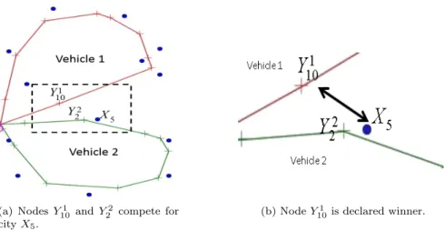
13 Example of node competition with bias term; assume that vehicle 2 is over-loaded and vehicle 1 is not. . . 46

14 General structure of fuzzy logic controller [32] . . . 50

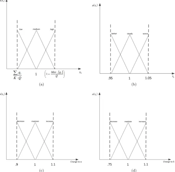
15 Triangular membership functions used in FLC. The fuzzification process uses 15a and 15b, and the defuzzification process uses 15c and 15d. . . 54

16 Rice’s [3] original diagram of the algorithm selection model. . . 64

17 Rice’s enhanced algorithm selection model to include the feature space [6]. . 64

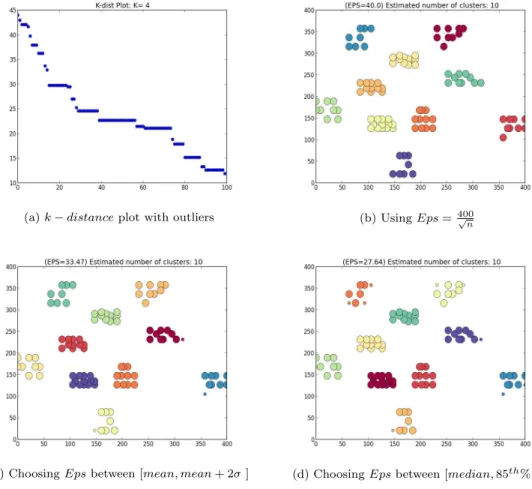
18 Example of how to use thek−distanceplot to identify Eps. . . 70

19 n= 9 cities placed uniformly on a 400 x 400 grid. The distance fromci to its 4 nearest neighbors isd= 400₂ = 200. . . 71

20 Example of using Equation 40 to defineEpsparameter in DBSCAN. . . 71

21 5th degree polynomial fit to ak−distanceplot usingnumpy.polyfit in Python. 72 22 Comparing the relationship between the ‘valley’ in the curve and the inflec-tion point. The approximate inflecinflec-tion point is found in the yellow rectangle, whereas the first ‘valley’ is located in one of the red circles. . . 73

Figure Page

23 Example of the difference between the approximate locations of the inflection

point and ‘valley’ in the fittedk−distancecurve. . . 73

24 Choosing Eps from values within 2 standard deviations above the mean is ineffective in the presence of largek−distanceoutliers. . . 75

25 ChoosingEps where all three methods yield similar results. . . 76

26 ChoosingEps where choosingEps using Equation 40 is not sufficient. . . 77

27 ChoosingEps where the method of choosingEps between [mean, mean+ 2σ ] is not sufficient. . . 78

28 number of clusters . . . 89

29 proportion of distinct distances . . . 89

30 Histograms of each algorithms performance, measured by PDB, across all benchmark problems . . . 90

31 Scatter plots of algorithm performance (percent deviation above best known solution) versus the number of cities in the problem . . . 92

32 The codebook vectors of the trained SOM based on the 102 benchmark prob-lem sets . . . 94

33 Plot of the average distance between a node and its neighbors . . . 94

34 Plot of the number of input vectors that are mapped to each node . . . 94

35 K means plot to identify the ‘elbow’ in the curve . . . 95

36 Trained SOM with six clusters . . . 95

37 SOM component plane: number of cities . . . 97

38 SOM component plane: ratio of the number of clusters to the number of cities 97 39 SOM component plane: number of clusters . . . 97

40 SOM component plane: y-coordinate of the depot . . . 97

41 102 benchmark problems mapped to the trained SOM . . . 98

42 Best performing algorithm for each problem instance mapped to the trained SOM where circle=C& W, triangle=Sweep, and plus sign=Fuzzy SOM . . . 98

43 Codebook vectors of the trained SOM . . . 99

44 Average distance between a node and its neighboring nodes . . . 99

Figure Page

46 Mapping of the best algorithm for each of the problem instances in thetraining

set . . . 99

.47 Number of Cities . . . 119

.48 Standard Deviation of the Distance Matrix . . . 119

.49 X-coordinate of City Centroid . . . 119

.50 Y-coordinate of City Centroid . . . 119

.51 Radius of Problem Instance . . . 120

.52 Proportion of Distinct Distances . . . 120

.53 Standard Deviation of the Nearest Neighbor Distances . . . 120

.54 Coefficient of Variation for Nearest Neighbor Distances . . . 120

.55 Ratio of the Number of Clusters to the Number of Cities . . . 121

.56 Ratio of the Number of Outliers to the Total Number of Cities . . . 121

.57 Ratio of the Number of Edge Cities to Total Number of Cities . . . 121

.58 Number of Clusters . . . 121

.59 Mean Radius of the Clusters . . . 122

.60 X-coordinate of the Depot . . . 122

.61 Y-coordinate of the Depot . . . 122

.62 Standard Deviation of Demand . . . 122

.63 Ratio of Total Demand to Total Vehicle Capacity . . . 123

.64 Ratio of the Max Cluster Demand to Vehicle Capacity . . . 123

.65 Ratio of Outlier Demand to Overall Demand . . . 123

.66 Ratio of the Maximum City Demand to Vehicle Capacity . . . 123

.67 Average Number of Customers Per Route . . . 124

.68 Area of the Rectangle . . . 124

.69 Minimum Number of Trucks . . . 124

.70 Scatter plots of algorithm performance (percent deviation above best known solution) versus the number of cities in the problem . . . 125 .71 Scatter plots of algorithm performance (percent deviation above best known

Figure Page

.72 Scatter plots of algorithm performance (percent deviation above best known solution) versus the x coordinate of the instance centroid . . . 127 .73 Scatter plots of algorithm performance (percent deviation above best known

solution) versus the y coordinate of the instance centroid . . . 128 .74 Scatter plots of algorithm performance (percent deviation above best known

solution) versus the radius of the problem instance . . . 129 .75 Scatter plots of algorithm performance (percent deviation above best known

solution) versus the proportion of distinct distances in the distance matrix (rounded to two decimal values) . . . 130 .76 Scatter plots of algorithm performance (percent deviation above best known

solution) versus the standard deviation of the nearest neighbors . . . 131 .77 Scatter plots of algorithm performance (percent deviation above best known

solution) versus the coefficient of variation of the nearest neighbors . . . 132 .78 Scatter plots of algorithm performance (percent deviation above best known

solution) versus the ratio of clusters to the total number of cities for each problem instance . . . 133 .79 Scatter plots of algorithm performance (percent deviation above best known

solution) versus the ratio of outliers to the total number of cities for each problem instance . . . 134 .80 Scatter plots of algorithm performance (percent deviation above best known

solution) versus the ratio of cities at the edge of a cluster (identified by DB-SCAN) to the total number of cities for each problem instance . . . 135 .81 Scatter plots of algorithm performance (percent deviation above best known

solution) versus the number of clusters found by DBSCAN for each problem instance . . . 136 .82 Scatter plots of algorithm performance (percent deviation above best known

solution) versus the mean radius of the clusters for each problem instance . . 137 .83 Scatter plots of algorithm performance (percent deviation above best known

solution) versus the x coordinate of the depot for each problem instance . . . 138 .84 Scatter plots of algorithm performance (percent deviation above best known

solution) versus the y coordinate of the depot for each problem instance . . . 139 .85 Scatter plots of algorithm performance (percent deviation above best known

solution) versus the standard deviation of the demand for each problem instance140 .86 Scatter plots of algorithm performance (percent deviation above best known

solution) versus the ratio of total demand to the available capacity (based on the minimum number of trucks required for the problem) for each problem instance . . . 141

Figure Page

.87 Scatter plots of algorithm performance (percent deviation above best known solution) versus the ratio of the largest cluster demand to a single vehicle’s

capacity for each problem instance . . . 142

.88 Scatter plots of algorithm performance (percent deviation above best known solution) versus the ratio of sum of all outlier demands to the overall demand for each problem instance . . . 143

.89 Scatter plots of algorithm performance (percent deviation above best known solution) versus the ratio of the single largest city demand to the vehicle ca-pacity for each problem instance . . . 144

.90 Scatter plots of algorithm performance (percent deviation above best known solution) versus the average number of customers per route for each problem instance . . . 145

.91 Scatter plots of algorithm performance (percent deviation above best known solution) versus the area of the rectangle that all problems lie within for each problem instance . . . 146

.92 Scatter plots of algorithm performance (percent deviation above best known solution) versus the minimum number of trucks required for each problem instance . . . 147

.93 SOM component plane: number of cities . . . 148

.94 SOM component plane: standard deviation of the distance matrix . . . 148

.95 SOM component plane: x-coordinate of city centroid . . . 148

.96 SOM component plane: y-coordinate of city centroid . . . 148

.97 SOM component plane: radius of problem instance . . . 148

.98 SOM component plane: proportion of distinct distances . . . 148

.99 SOM component plane: standard deviation of the nearest neighbor distances 149 .100 SOM component plane: coefficient of variation for nearest neighbor distances 149 .101 SOM component plane: ratio of the number of clusters to the number of cities 149 .102 SOM component plane: ratio of the number of outliers to the total number of cities . . . 149

.103 SOM component plane: ratio of the number of edge cities to total number of cities . . . 149

.104 SOM component plane: number of clusters . . . 149

.105 SOM component plane: mean radius of the clusters . . . 149

Figure Page

.107 SOM component plane: y-coordinate of the depot . . . 150 .108 SOM component plane: standard deviation of demand . . . 150 .109 SOM component plane: ratio of total demand to total vehicle capacity . . . . 150 .110 SOM component plane: ratio of the max cluster demand to vehicle capacity . 150 .111 SOM component plane: ratio of outlier demand to overall demand . . . 150 .112 SOM component plane: ratio of the maximum city demand to vehicle capacity 150 .113 SOM component plane: average number of customers per route . . . 150 .114 SOM component plane: area of the rectangle . . . 150 .115 SOM component plane: minimum number of trucks . . . 151 .116 Histograms of the number of cities in both the existing benchmark problem

set and the newly generated problem set . . . 152 .117 Histograms of the standard deviation of the distance matrix in both the

exist-ing benchmark problem set and the newly generated problem set . . . 153 .118 Histograms of the x-coordinate of the centroid in both the existing benchmark

problem set and the newly generated problem set . . . 153 .119 Histograms of the y-coordinate of the centroid in both the existing benchmark

problem set and the newly generated problem set . . . 154 .120 Histograms of the problem radius in both the existing benchmark problem set

and the newly generated problem set . . . 154 .121 Histograms of the proportion of distinct distances in the distance matrix in

both the existing benchmark problem set and the newly generated problem set 155 .122 Histograms of the standard deviation of the nearest neighbors in both the

existing benchmark problem set and the newly generated problem set . . . . 155 .123 Histograms of the problem radius in both the existing benchmark problem set

and the newly generated problem set . . . 156 .124 Histograms of the ratio of the number of clusters to the number of cities in

both the existing benchmark problem set and the newly generated problem set 156 .125 Histograms of the ratio of the number of outliers to the number of cities in

both the existing benchmark problem set and the newly generated problem set 157 .126 Histograms of the ratio of the number of cities on the edge of a cluster to the

total number of cities in both the existing benchmark problem set and the newly generated problem set . . . 157 .127 Histograms of the number of clusters in both the existing benchmark problem

Figure Page

.128 Histograms of the mean radius of the clusters in both the existing benchmark

problem set and the newly generated problem set . . . 158

.129 histograms of the x-coordinate of the depot in both the existing benchmark problem set and the newly generated problem set . . . 159

.130 Histograms of the y-coordinate of the depot in both the existing benchmark problem set and the newly generated problem set . . . 159

.131 Histograms of the standard deviation of demand in both the existing bench-mark problem set and the newly generated problem set . . . 160

.132 Histograms of the ratio of the total demand to the total vehicle capacity in both the existing benchmark problem set and the newly generated problem set 160 .133 Histograms of the ratio of the maximum cluster demand to vehicle capacity in both the existing benchmark problem set and the newly generated problem set 161 .134 Histograms of the ratio of the outlier demand to the total demand in both the existing benchmark problem set and the newly generated problem set . . . . 161

.135 Histograms of the ratio of the maximum demand to the vehicle capacity in both the existing benchmark problem set and the newly generated problem set 162 .136 Histograms of the average number of customers per route in both the existing benchmark problem set and the newly generated problem set . . . 162

.137 Histograms of the area of the rectangle the cities lie within for both the existing benchmark problem set and the newly generated problem set . . . 163

.138 Histograms of the minimum number of trucks required in both the existing benchmark problem set and the newly generated problem set . . . 163

.139 K-means plot for the trained SOM for prediction . . . 167

.140 8 clusters in the trained SOM for prediction . . . 167

.141 SOM component plane: number of cities . . . 168

.142 SOM component plane: standard deviation of the distance matrix . . . 168

.143 SOM component plane: x-coordinate of city centroid . . . 168

.144 SOM component plane: y-coordinate of city centroid . . . 168

.145 SOM component plane: radius of problem instance . . . 168

.146 SOM component plane: proportion of distinct distances . . . 168 .147 SOM component plane: standard deviation of the nearest neighbor distances 168 .148 SOM component plane: coefficient of variation for nearest neighbor distances 168 .149 SOM component plane: ratio of the number of clusters to the number of cities 169

Figure Page

.150 SOM component plane: ratio of the number of outliers to the total number of

cities . . . 169

.151 SOM component plane: ratio of the number of edge cities to total number of cities . . . 169

.152 SOM component plane: number of clusters . . . 169

.153 SOM component plane: mean radius of the clusters . . . 169

.154 SOM component plane: x-coordinate of the depot . . . 169

.155 SOM component plane: y-coordinate of the depot . . . 169

.156 SOM component plane: standard deviation of demand . . . 169

.157 SOM component plane: ratio of total demand to total vehicle capacity . . . . 170

.158 SOM component plane: ratio of the max cluster demand to vehicle capacity . 170 .159 SOM component plane: ratio of outlier demand to overall demand . . . 170

.160 SOM component plane: ratio of the maximum city demand to vehicle capacity 170 .161 SOM component plane: average number of customers per route . . . 170

.162 SOM component plane: area of the rectangle . . . 170

CHAPTER 1 Introduction

This research is motivated by the intersection of combinatorial optimization and artificial neural networks. The most basic underlying question is how the strengths of artificial neural networks can be used to solve inherently difficult combinatorial optimization problems. This introductory chapter provides a brief overview of both combinatorial optimization and artificial neural networks. Chapters 2 and 3 provide a detailed background of the Vehicle Routing Problem (which is the specific combinatorial optimization problem this research is focused on), as well as the existing artificial neural network approaches to solving the vehicle routing problem. Chapter 4 introduces an updated artificial neural network approach to solving the vehicle routing problem, along with the experimental results and discussion. Chapter 5 uses a SOM as a tool for analyzing the diversity of CVRP benchmark problems, as well as a prediction tool for choosing the best performing algorithm for a new CVRP problem instance. Chapter 6 provides the conclusion as well as directions for future work.

1.1 Optimization

Optimization problems deal with maximizing or minimizing a function, normally of many variables and subject to constraints. In general, optimization problems can be divided into two categories: problems with continuous variables and problems with discrete variables. An optimization problem whose solution can be found within a finite set of possible solutions is called a combinatorial optimization problem [1].

The practicality of combinatorial optimization problems (COPs) to everyday life cannot be overstated. Combinatorial optimization problems exist across a wide range of disciplines and are solved on a daily basis. In his overview of the early history of combinatorial optimization, Schrijver [2] suggests primitive examples of COPs such as searching for food or short paths, as well as more modern applications such as creating a mailman’s route, assigning jobs amongst people, and the transporting of goods. Although combinatorial optimization emerged as its own field of study in the middle of the twentieth century, the roots of many problems can be traced back decades or even centuries [2].

The study of solving combinatorial optimization problems is deeply intertwined with the study of computational complexity. Computational complexity refers to the categorization of

Figure 1: Comparison of various polynomial and exponential time complexity functions [4].

problem difficulty based on the efficiency of computer methods for solving these problems [3]. Although an in depth discussion ofP versusN Pis beyond the scope of this thesis, it is important to note that many combinatorial optimization problems areN P-Hard. This indicates that there is not a known, polynomial time algorithm that can find the optimal solution.

In the study of computational complexity, algorithms are generally described as either a polynomial time algorithm or an exponential time algorithm. A polynomial time algorithm is an algorithm in which the time complexity function can be expressed in terms of a polynomial, whereas anexponential time algorithm cannot. Additionally, anexponential time algorithmdoes not necessarily have to be an exponential function, it is just not a polynomial function. For example, an algorithm with a time complexity function ofnlognis considered anexponential time algorithm [4].

The importance of time complexity function is illustrated in 1. As seen in this table provided by Garey and Johnson [4], it is clear that as the problem size,n, increases, it is not feasible to useexponential time algorithms for solving these problems. For the numerousN P-hard combi-natorial optimization problems, this is the case. There are currently no known,polynomial time algorithms for solving theseN P-hard problems. Therefore a great deal research into combina-torial optimization focuses on heuristic algorithms.

1.2 Artificial Neural Networks

The study of Artificial Neural Networks (ANNs) is inspired by the organization and func-tions of the biological neural networks in the human brain [5]. At the core of ANN research is the recognition that although the performance of modern computers is superior to that of humans for computational tasks, the relative ease at which the human brain can process and solve complex tasks dominates even the best computers. Jain and Mao [6] describe many of the superior, inher-ent capabilities of the human brain as compared to the modern computer: massive parallelism, distributed representation and computation, learning ability, generalization ability, adaptivity, inherent contextual information processing, fault tolerance, and low energy consumption. In the study of ANNs, the goal is to simulate functions of the brain with a computer in order to exploit these capabilities.

Scientists across many disciplines have developed various ANNs in order to solve problems such as: pattern classification, speech synthesis and recognition, adaptive interfaces between humans and complex physical systems, function approximation, image data compression, as-sociative memory, clustering, forecasting and prediction, combinatorial optimization, nonlinear system modeling, and control [7]. While researchers have found success in the application of ANNs to many of these problems, their application to optimization has been less successful [8].

1.3 Combinatorial Optimization and Artificial Neural Networks

Simply put, an ANN is a heuristic. It is a method, modeled after the human brain, used to find a good solution to a problem. Since the solvability of real-world sized combinatorial optimization problems relies almost exclusively on heuristics, it is reasonable to question whether ANNs are, or can be developed, as useful tools for solving these combinatorial optimization problems. To date, the most widely studied combinatorial optimization problem that ANN research has focused on is the Traveling Salesman Problem (TSP), with the Vehicle Routing Problem (VRP) being the second most studied [9]. The most current literature indicates that ANNs are inferior to the best heuristics for the TSP as well as the VRP [10, 11]. Although this has created pessimism in some researchers, other researchers encourage continued research in these areas [10, 11] with the belief that small changes, over time, can lead to large changes; as well as the belief that advances in this work might be beneficial to other research areas; and that ANNs might become competitive with the availability of massively parallel computers.

List of References

[1] C. H. Papadimitriou and K. Steiglitz, Combinatorial Optimization: Algorithms and Com-plexity. Courier Dover Publications, 1998.

[2] S. Alexander, “On the history of combinatorial optimization (till 1960),” Handbooks in Operations Research and Management Science: Discrete Optimization, vol. 12, p. 1, 2005. [3] E. A. Lamagna, “Infeasible computation: Np-complete problems,” ABACUS, vol. 4, no. 3,

pp. 18–33, 1987.

[4] M. R. Garey and D. S. Johnson,Computers and Intractability. wh freeman, 2002, vol. 29. [5] J. Brownlee, Clever algorithms: nature-inspired programming recipes. Jason Brownlee,

2011.

[6] A. K. Jain, J. Mao, and K. Mohiuddin, “Artificial neural networks: A tutorial,”Computer, vol. 29, no. 3, pp. 31–44, 1996.

[7] M. H. Hassoun,Fundamentals of artificial neural networks. MIT press, 1995.

[8] I. H. Osman and G. Laporte, “Metaheuristics: A bibliography,” Annals of Operations Re-search, vol. 63, no. 5, pp. 511–623, 1996.

[9] M. Schwardt and J. Dethloff, “Solving a continuous location-routing problem by use of a self-organizing map,” International Journal of Physical Distribution & Logistics Management, vol. 35, no. 6, pp. 390–408, 2005.

[10] E. Cochrane and J. Beasley, “The co-adaptive neural network approach to the euclidean travelling salesman problem,”Neural Networks, vol. 16, no. 10, pp. 1499–1525, 2003. [11] J.-C. Cr´eput and A. Koukam, “The memetic self-organizing map approach to the vehicle

CHAPTER 2

The Vehicle Routing Problem 2.1 Origin

The Vehicle Routing Problem (VRP) consists of finding the optimal routing of a fleet of vehicles amongst a set of cities, where each city has a demand for goods that the vehicles must deliver, and each vehicle has a constraint on the capacity of goods it can transport. Examples of the VRP include the distribution of goods such as in the beverage or food industries, the collection of waste, or the delivery of mail or newspapers [1]. The applications of the VRP span many industries, each with its own unique attributes, which have resulted in many variations of Vehicle Routing Problems.

The VRP was first introduced as the Truck Dispatching Problem in 1959 [2]. In their original work on this problem, Dantzig and Ramser introduced the Truck Dispatching Problem as a generalization of the Traveling Salesman Problem (TSP). Although the term ‘traveling salesman problem’ became relevant in the mathematics community in the early 1930’s [3], William Cook provides an extensive history of the TSP prior to its formal entrance into the mathematics field, which goes back nearly two centuries, in his bookIn Pursuit of the Traveling Salesman [4] .

Given a set of cities, the objective of the TSP is to find the shortest route of visiting all the cities and returning to the starting point. Dantzig and Ramser generalize the TSP to introduce the Truck Dispatching Problem by specifying that deliveries be made at each one of the cities. Furthermore, the carrier of these deliveries is constrained by the capacity it can transport in one load. If there is only one truck (carrier) with an infinite capacity, this is simply the TSP.

In the initial introduction of the Truck Dispatching Problem, the authors spent the majority of the paper discussing one variant of the problem. In their problem formulation, Dantzig and Ramser assumed that for the fleet of vehicles and set cities, ‘only one product is to be delivered and that all trucks have the same capacityC’ [2]. This formulation of the problem has subsequently become the most widely studied variant of Vehicle Routing Problems [5], and this formulation is referred to as the Capacitated Vehicle Routing Problem (CVRP). From the original introduction as the Truck Dispatching Problem, however, the Vehicle Routing Problem literature consists of numerous variations of the general problem. In addition to the CVRP, additional problems which have received a great deal of attention in the literature [5] are as follows:

• The Distance Constrained VRP

• The VRP with Time Windows

• The VRP with Backhauls

• The VRP with Pickups and Delivery This research is focused on the CVRP.

2.2 Problem Formulation

As previously stated, this research focuses on the CVRP. Within the CVRP, there are two general variations. One in which the distances or costs associated with each arc (connection between nodes) are symmetric, and in the other case, these distances or costs are asymmetric. This research is specifically concerned with the symmetric CVRP, which is described as the following graph theoretic problem. Let G = (V, A) be an undirected, complete graph, where

V ={0, . . . , n} is the set of nodes, and A is the set of arcs which connect the nodes. A cost,

cij, is associated with each arc, (i, j) ∈ A, where i 6= j. In this research the cost associated

with each arc is simply the Euclidean distance between the nodes i and j, and because the problem is symmetric,cij =cji. Node 0 corresponds to the depot, whereas the remaining nodes,

V0 = V \ {0}, correspond to the customers. Each customer i ∈ V0 has a deterministic, non-negative demand,di, for goods. The goods are transported between the depot and the customers

by one of vehicles in the known, homogeneous set ofK vehicles. Each vehicle has a maximum capacity, Q, that is identical across the set of vehicles, anddi ≤Qfor each i= 1, . . . , n. The

objective of the CVRP is to find K vehicle routes that start and end at the depot, with the minimum cost, where the demand of each customer is met, and the capacity of each vehicle is not violated.

2.2.1 Mathematical Programming Formulations

As described by Toth and Vigo [5], there are three general ways that the CVRP has been modeled in the literature. These three approaches are: the vehicle flow formulation, the commod-ity flow formulation, and the set partitioning formulation. Within each of these formulations, there are numerous variations and extensions. The three basic models are described below, and in each formulation, the graphG(V, A) is assumed to be a complete graph. In line with the graph theoretic description,di is the demand associated with each city i; and given a set S ⊆V, the

total demand for the set isd(S) =X

i∈S

di. The formulations found in [5] follow.

Vehicle Flow Formulation

The basicvehicle flow formulation usesn2 _{binary variables,x}

ij, which correspond to each

arc (i, j)∈A. If the arc (i, j) is in the optimal solution,xij= 1, otherwise,xij = 0.

minX i∈V X j∈V cijxij (1) subject to: X i∈V xij = 1 ∀j∈V \ {0}, (2) X j∈V xij = 1 ∀i∈V \ {0}, (3) X i∈V xi0=K, (4) X j∈V x0j =K, (5) X i /∈S X j∈S xij ≥r(S) ∀S⊆V \ {0}, S6=∅, (6) xij ∈ {0,1} ∀i, j∈V. (7)

The first two constraints, equations 2 and 3, ensure that each customer vertex has precisely one arc entering and leaving. The next two constraints, equations 4 and 5, ensure that exactly

K (which corresponds to the number of vehicles) arcs enter and leave the depot vertex. The next constraint, equation 6, ensures that the solution routes are connected and that the capacity constraints are met. For a set S ⊆ V \ {0}, the term r(S) refers to the minimum number of vehicles required to serve all of the customers inS, based upon the total demand of the set,d(S). The term r(S) is the optimal solution to the Bin Packing Problem, which is also anN P-hard optimization problem. A valid [6] and common [5] substitute forr(S) in the above formulation is the lower bound of the Bin Packing Problemdd(_QS)e.

The abovevehicle flow formulation is a basic model for an asymmetric CVRP. The vehicle flow formulation is easily refined for the symmetric CVRP (which is the focus of the current research) as follows:

min X i∈V\{n} X j≥i cijxij (8) subject to: X h≤i xhi+ X j≥i xij= 2 ∀i∈V \ {0}, (9) X j∈V\{0} x0j= 2K, (10) X i∈S X h≤i h /∈S xhi+ X i∈S X j≥i j /∈S xij ≥2r(S) ∀S∈V \ {0}, S6=∅, (11) xij ∈ {0,1} ∀i, j∈V \ {0}, i≤j, (12) x0j ∈ {0,1,2} ∀j∈V \ {0}. (13)

The symmetric CVRP vehicle flow formulation stems from the TSP formulation from Dantzig, et al [7], which was then extended to the symmetric CVRP formulation in [8, 9]. In the symmetric formulation of the problem,cij=cji, therefore the decision variablexij can take on a

value of{0,1,2}, which represents the number of times that the arc is traversed in the final solu-tion. In the case of a route with only one customer,cij = 2 since the (i, j) arc must be traversed

twice in order to travel to and from the customer. The first constraint in the symmetric CVRP formulation, equation 9, is a combination of the first two constraints, equation 2 and equation 3, in the asymmetric formulation. This new constraint ensures that there is exactly one arc en-tering and one arc leaving each vertex (not including the depot vertex). The second constraint, equation 10, ensures that there is one arc entering and one arc exiting the depot vertex for each of theKvehicles in the problem. The third constraint, equation 10, ensures the continuity of the solution, as well as enforcing that the vehicle capacity constraints are not violated by requiring an adequate number of edges to enter each subset of vertices.

In addition to different versions of the vehicle flow formulation for the asymmetric and symmetric CVRP, additional versions and variations exist. Toth and Vigo [5] provide a detailed overview of the extensions and modifications of this model. One of the most notable extensions is the three index model [10, 11], which uses a binary variablexijk which is equal to 1 if vehicle

Commodity Flow Formulation

The first application of thecommodity flow model was to an oil delivery problem [12]. Sub-sequent work [13, 14, 5] extended the model to both the TSP and VRP. These early formulations of thecommodity flow formulation are detailed in [15]. And a more recent example by Baldacci, et al [16] extends the TSP model introduced by Finke, et al [17].

The commodity flow formulation deals with an extended graph G0 = V0, A0. In this extended graph,V0 =V∪{n+1}where{n+1}is a copy of the depot, andA0 =A∪{(i, n+ 1) :i∈

V}. As with the previously described model, the binary variables,xij, correspond to arc (i, j). If

the arc (i, j) is in the optimal solution, xij = 1, otherwise,xij = 0. In addition to the variables

introduced in thevehicle flow formulation, thecommodity flow formulation introduces two new variables, yij and yji. If a vehicle travels along arc (i, j), the variable yij corresponds to the

vehicle’s load as it travels this arc, and the variableyjicorrpesonds to the available capacity on

the vehicle as it travels arc (i, j). For each arc (i, j)∈A0,yij+yji=Q, whereQis the maximum

capacity of the vehicle.

Toth and Vigo [5] describe the flow variablesyij andyjias representing two directed paths

through the solution. One path starts at the depot vertex, 0, and travels to the last vertexn+ 1. The variables on this path,yij, represent the vehicle load. The vehicle leaves the depot with a

load equal to the sum of all customers’ demands for the route. At each customer, the appropriate demand is delivered, and the vehicle ends at noden+ 1 empty. The second path starts at vertex

n+ 1 and travels to the depot vertex, 0. This second path can be described as the vehicle leaving vertexn+ 1 empty, and at each customer, the demand,di is picked up by the vehicle. Therefore,

when the vehicle arrives at the depot vertex, 0, the vehicle’s load is equal to the total demand of all the customers along the path. Figure 2 illustrates the variablesyij andyjifor an example

route with four cities, whereQ= 25 [5]. Each city’s demand is listed by the vertex. The following is thecommodity flow formulation for the symmetric CVRP.

Figure 2: Example to illustrate the variablesyij andyji on a route [5]. min X (i,j)∈A cijxij (14) subject to: X j∈V0 (yji−yij) = 2di ∀i∈V 0 \ {0, n+ 1}, (15) X j∈V0\{0,n+1} y0j=d(V \ {0, n+ 1}), (16) X j∈V0\{0,n+1} yj0=KQ−d(V \ {0, n+ 1}), (17) X j∈V0\{0,n+1} yn+1j =KQ, (18) yij+yji=Qxij ∀(i, j)∈A 0 , (19) X j∈V0 (xij+xji) = 2 ∀i∈V 0 \ {0, n+ 1}, (20) yij ≥0 (i, j)∈A 0 , (21) xij∈ {0,1} ∀(i, j)∈A 0 . (22)

The constraints in Equations 15 - 18 ensure the appropriate flow between the depot vertex 0 and the vertexn+ 1. The next constraint, in Equation 19, ensures feasible values foryij and

yji. The vehicle load along arc (i, j) plus the available capacityyj,i along arc (i, j) must always

equal the vehicle’s total capacityQ. And the constraint in Equation 20 ensures the continuity of the solution.

Set Partitioning Formulation

Theset partitioning formulation of the VRP was introduced in 1964 by Balinski and Quandt [18]. It is possible for this model to require an exponential number of binary variables. Each binary variable,xj, j= 1, . . . , r, is associated with one of therfeasible circuits ofG. A feasible

circuit is a subset of vertices of V that does not violate the capacity constraint. The variable

xj = 1 if the circuit is included in the final solution, andxj= 0 otherwise. Each of thercircuits

has a minimum cost associated with itc∗_j; and a binary variableaij= 1 if vertexiis included in

circuitj. min r X j=1 c∗_jxj (23) subject to: r X j=1 aijxj = 1 ∀i∈V \ {0}, (24) r X j=1 xj=K, (25) xj ∈ {0,1} ∀j= 1, . . . , r. (26) (27)

The first constraint, Equation 24, ensures that each vertex is included in the solution, and the second constraint, Equation 25, requires exactlyK circuits (vehicle routes) in the solution. It is important to note that findingc∗_j is, itself, anN P-hard optimization problem [19].

2.3 Approaches to Solving CVRP

As previously described, the CVRP is an N P-hard, which makes it difficult to solve to optimality for a non-trivial sized problem. The two general categories of algorithms used to solve the CVRP are exact algorithms and heuristic algorithms. Exact algorithms are concerned with finding the optimal solution to the CVRP, whereas heuristics are concerned with finding a good solution, but not necessarily the optimal.

2.3.1 Exact Algorithms

To date, the largest CVRP that has been solved to optimality consists of 134 cities [20, 21, 22, 23, 16]. Even though there have been significant advances in exact methods for solving the CVRP in the past 50 years, the existing exact methods are not yet capable of reliably solving

real-world-sized vehicle routing problems [19]. The earliest survey of exact methods for solving the VRP was the work by Laporte and Norbert [15]; which has been subsequently updated in 2002 [5], 2007 [24, 25]; 2008 [26], and 2010 [20]. Due to the limitations of these exact methods, the majority of VRP research focuses on heuristics [27].

2.3.2 Heuristic Methods

The first heuristic proposed for solving the VRP was introduced by Dantzig and Ramser with their initial introduction of the ‘Vehicle Dispatching Problem’ [2]. Since the introduction of the VRP, a significant amount of research has focused on heuristics methods for solving the

N P −hardproblem. The VRP heuristic literature is immense, and an extensive review of VRP heuristics can be found in [5, 28, 29].

VRP heuristics can be broadly divided into two categories: classical heuristics, and meta-heuristics [27]. A general overview of these two categories follows.

Classical Heuristics

Classical heuristics are described as methods that do not make a deep exploration of the search space, have fairly short computing times, and are capable of producing fairly good quality solutions [30]. Laporte [27] further describes classical heuristics with the fact that every step of the heuristic is a decent, which means that the heuristic never allows inferior solutions (even temporarily). These classical heuristics only move from one solution if the subsequent solution is superior. Classical heuristics are often divided into two categories: constructive and improvement heuristics.

Constructive Heuristics Constructive heuristics solve a problem by progressively building the routes. As the heuristic builds the solution, it monitors the cost, and ensures that the solution remains feasible. Three of the most widely known constructive heuristics are the Clarke and Wright algorithm, the sweep algorithm, and the Fisher and Jaikumar algorithm.

Clarke and Wright Savings Algorithm

One of the best known constructive heuristics is the Clarke and Wright Savings Algorithm [31]. This algorithm was introduced in 1964 and is still popular today [19]. The algorithm begins with n feasible routes, one back and forth route between the depot and each customer. On a given iteration, two routes (0, . . . , i, . . . ,0) and (0, . . . , j, . . . ,0) can be merged together if the resulting route (0, . . . , i, j, . . . ,0) is feasible with regard to the capacity constraint. If these routes

are merged, there is a savings ofsij =ci0+c0j−cij. The algorithm has two versions: a parallel

implementation and a sequential implementation.

Both the parallel and sequential versions of the algorithm are initialized identically. The first step is to create a vehicle route, (0, i,0) for each city, i ∈V \ {0}. Next, a list of savings

sij =ci0+c0j−cij for each (i, j)∈Awhere i6=j is created. After the creation of the savings

list, the steps of the parallel and sequential versions of the algorithm diverge.

In the parallel version of the algorithm, the next step consists of identifying the largest savings,sij in the savings list; followed by the determination of whether the two routes can be

feasibly merged. If the two routes from the savings list, one containing the edge (i,0) and the other containing the edge (0, j), can be feasibly merged, the two routes are combined resulting in a new route consisting of the edge (i, j). In this parallel version, multiple routes are being developed at the same time. This process continues until allsij have been inspected for potential

route merging.

In the sequential version of the algorithm, after the creation of thenroutes and the savings list, each route is fully expanded before the next route is considered. To accomplish this, one route (0, i, . . . , j,0), is considered at a time. The current route is merged with another route that contains the largest savings,skiorsjl, that can be feasibly merged with the current route. This

process continues for the current route, until there are no more feasible merges. Then the next route is considered.

Several modifications have been introduced for the Clarke and Wright algorithm since its debut in 1964. One of the limitations of the Clarke and Wright algorithm is its tendency for the quality of the route construction to deteriorate near the end of the algorithm [30]. To overcome this, a shape parameter was introduced to the savings calculations by Gaskell [32] and Yellow [33], and subsequent work into the appropriate settings for this shape parameter was presented by Golden, et al [10]. The incorporation of a matching algorithm was introduced by Desrochers and Verhoog [34] as well as Altinkemer and Gavish [35] with the intent of optimizing the route merges at each iteration of the algorithm. Finally, enhancements to improve the computational time were presented by Paessens [36]; and Nelson et al [37], introduced efficient data structure usage. An in depth survey of the various modifications to the Clarke and Wright algorithm can be found in [30].

Sweep Algorithm

algorithm was introduced by Gillet and Miller [38] as a way to divide a large VRP into smaller subproblems. To implement the sweep algorithm, each city (node) must be represented by its polar coordinates (θi, ri). The plane is centered at the depot, and one city,i∗is chosen such that

θ∗_i = 0. The polar coordinates for the remaining cities are found accordingly.

The cities are then ordered, by their increasing polar angle values. Starting with the first vehicle, k = 1, and the unrouted city with the smallest polar angle (the top of the city list), cities are assigned to vehicle k = 1 until the capacity of the vehicle has been met. Once the vehicle capacity is met, the next vehicle is initialized, k = 2, and the unrouted city with the smallest polar angle is assigned to this vehicle. Moving down the list of cities, a city is added to the current vehicle, k, until the vehicle capacity has been met, at which point a new vehicle is initialized and the process continues. The algorithm halts once all cities are assigned to a vehicle. Once the cities have been partitioned amongst thekvehicles, each vehicle’s route is found by solving the corresponding TSP. The TSP can be solved exactly or approximately. This sweep algorithm is sometimes referred to as a two phase method, which refers to the fact that one phase of the algorithm is devoted to clustering or partitioning the cities, and the other phase is concerned with the vehicle’s route amongst these cities.

Fisher and Jaikumar Algorithm

The last well known classical heuristic that is discussed is the Fisher and Jaikumar algorithm [11]. Instead of relying on the geometric nature of the problem to form the clusters, the Fisher and Jaikumar algorithm first solves a Generalized Assignment Problem in order to divide the cities amongst thekvehicles. Similar to the sweep algorithm, the Jaikumar and Fisher algorithm is also commonly referred to as a two phase method, due to the fact that the tasks of clustering the cities and finding the routes are completed in two separate steps.

The first step of the algorithm is to identify k seed vertices jk ∈ V. Each of these seeds

corresponds to one of theKvehicle routes. Once these seeds are identified, a cost for allocating a customer,i, to each route,k, is computed: dik= min{c0i+cijk+cjk0, c0jk+cjki+ci0}−(c0jk+cjk0).

Next, the generalized assignment problem is solved withdik as the costs, the customer weights

qi, and the vehicle capacity Q. Once all customers are assigned to a route resulting from the

generalized assignment problem, a TSP is then solved to find the optimal routing for each vehicle.

Improvement Heuristics The second category of classical heuristics is improvement heuris-tics. Improvement heuristics for a VRP are applied to an existing solution. Often these

improve-ment heuristics are applied to the results of previously described classical heuristics [28]. With this existing solution, improvements can be made within individual routes, or across many routes at the same time.

Improvements made to a single route at a time, intra-route improvements, stem from the

λ−optTSP heuristic introduced by Lin and Kernighan [39]. Starting with a solution, theλ−opt

procedure removes λ edges from the solution and then reconnects the remaining segments of the solution in every possible combination. When a superior solution is found, the procedure is repeated, and this process continues until there are no further improvements. At this point, the solution is said to be λ−opt. Several improvements have been introduced to the λ−opt

method. Instead of setting aλvalue at the beginning of the algorithm, Lin and Kernighan suggest changingλdynamically while the algorithm is running [40]. Another modification presented by Or [41] entails removing and reinserting a chain of 3 vertices until no more improvements can be found, and this procedure is then repeated with chains of 2 vertices, followed by a single vertex. Additional modifications to intra-route improvement heuristics and modifications are described in [30, 42].

Improvements made across multiple routes are called inter-route improvements. Just as with an intra-route improvement, an inter-route improvement heuristic begins with a solution to the VRP. With this initial solution, an attempt is made to move cities/nodes amongst routes with the goal of finding a superior solution. Van Breedam [43] classifies inter-route improvement heuristics into four categories: string cross, string exchange, string relocation, and string mix. Van Breedam traces the main ideas of these heuristics to the previous work of Dror and Levy [44] and Savelsbergh [45]. Van Breedam’s inter-route improvement heuristics are briefly described as follows:

• The string cross move consists of crossing two arcs of two distinct routes. This is equivalent to the exchange of route segments between the routes (see Figure 3).

• The string exchange swaps two sets of Kvertices between routes. NormallyK = 1,2 (see Figure 4).

• The string relocation move shifts a string ofK vertices from one route to another. Just as with the string cross, normallyK= 1,2 (see Figure 5).

(a) String Cross before (b) string cross after

Figure 3: string cross

(a) String Exchange before (b) string exchange after

Figure 4: string exchange

One additional inter-route improvement heuristic to note is the work by Thompson and Psaraftis [46]. The authors develop a general b-cyclic, k-transfer system where k vertices are shifted to the next route in circular permutation ofbroutes. Additional inter-route improvements heuristics as well as modifications to the ones described can be found in [47, 48, 49, 50, 51, 30, 28].

2.3.3 Metaheuristics

The second general category for solving a CVRP is metaheuristics. Unlike classical heuristics, metaheuristics employ a deep search of the solution space [30], and they utilize concepts and procedures from the classical VRP heuristics [27]. In 1986 Fred Glover introduced the term

(a) String Relocation before (b) string relocation after

‘metaheuristic’ to describe a heuristic that can be described generally, but which employs more specific heuristics necessary for the specific problem at hand [52]. Glover went on to predict that this type of metaheuristic will become very useful for solving combinatorial optimization problems. Since the initial introduction, numerous metaheuristics have been developed for various combinatorial optimization problems.

Now, instead of developing algorithms for a specific problem from scratch, these metaheuris-tics can be tailored to a specific problem, or type of problems [29]. Many metaheurismetaheuris-tics have been shown to find nearly optimal solutions in an acceptable computation time for various com-binatorial optimization problems [53]. The implementation of metaheuristics specifically to the VRP have been extremely successful [29].

Due to the volume of metaheuristics introduced in the literature, this section does not provide a complete survey of all applications of metaheuristics to the VRP. The most recent detailed survey of metaheuristics for the VRP can be found in [29]. This section will focus on three broad categories of metaheuristics [24, 27, 19]: local search, population search, and learning mechanisms.

Local Search

A local search heuristics is initialized with a solution. A neighborhood is defined around the current solution, and at each iteration, the heuristic moves to a new solution in this neighborhood. The procedure terminates based on predefined stopping criteria and returns the best solution found throughout the search. Given this general framework, various algorithms can be developed [27]. Two examples of local search algorithms are the simulated annealing and tabu search.

Simulated Annealing

Simulated annealing (SA) was first introduced as a technique for optimization in 1983 [54]. The general form of simulated annealing is described by Gendreau, et al [55], as follows. At each iteration of the simulated annealing algorithm, a solution x is randomly taken from the neighborhood of the current solutionxt. If the cost of this neighboring solution is less than the

cost of the current solution, f(x) ≤f(xt), then the current solution is updated: xt+1 =x. If the cost of the neighboring solution is not an improvement, then the current solution is updated,

xt+1 =xwith a probability of pt; andxt+1 =xt, otherwise. The probability, pt is normally a

decreasing function of both the iteration,t, andf(x)−f(xt), and can be defined as:

In Equation 28, θt represents the ‘temperature’ at iteration t, and the rule that defines and

updates θt is called the ‘cooling schedule’. Normally θt is a decreasing function. As a result,

the probability of updating the current solution to a worse solution decreases over time. The algorithm’s stopping criteria usually depends on the number of iterations, or the frequency of updates toward a better solution.

This meta-strategy generally guides the algorithm, however, the specifics of how the neigh-borhood is searched, as well as how the cooling schedule is defined significantly impact the algorithm’s performance. One of the earliest and most successful implementations for the CVRP was by Osman in 1993 [48]. In his implementation, the algorithm was initialized with a solution found by the Clarke and Wright algorithm, and he employed similar inter and intra-route im-provement techniques described in the previous section. Osman’s simulated annealing algorithm resulted in generally good solutions, however, his computation times were rather long, and his results were not competitive with other location search heuristics, such as the tabu search.

Tabu Search

Another well known metaheuristic for the VRP is the tabu search, which can be traced back to Glover [52]. Similar to simulated annealing, the tabu search begins with an initial solution. At each iteration, the current solution is updated with the best solution found in the surrounding neighborhood, even if there is no improvement from the current solution. To avoid cycling amongst solutions, solutions that have been recently examined are marked as ‘tabu’ for a certain number of iterations. Again, whereas the general strategy across different tabu search algorithms is the same, the details of how the neighborhood is searched, the rules for updating solutions, and how the tabu routes are stored in memory are all factors that significantly influence a tabu search algorithm’s performance.

Gendreau, et al [55] describe the earliest applications of a tabu search to the VRP. Although the earliest work of Willard [56] in 1989 was improved upon by Pureza and Franca [57] just two years later, Gendreau et al describes neither implementation of having very good results. However, more refined search strategies led to significant improvements in the application of the tabu search to VRP.

In his 1993 paper, Osman not only outlined an SA approach to solving the CVRP, he also introduced a tabu search metaheuristic [48]. In his tabu search, Osman used the same inter and intra-route improvements as he did with his SA algorithm for the neighborhood search. For the tabu search, he tested two different schemes for updating the current solution. In one scheme, he

searched the entire neighborhood to find the best solution before updating the current solution. In the second scheme, he updated the current solution as soon as an admissible improvement was found. Only feasible and non-tabu solutions were considered for an update.

Gendreau, et al, soon improved upon many of the results of Osman with a more intricate tabu search algorithm for the CVRP, which they called TABUROUTE. The authors defined a neighborhood as all of the solutions that can be found by removing one vertex from the current solution and reinserting into a different route that contains one of the vertex’s nearest neighbors. This generalized insertion procedure, GENI, was previously created by the authors as a post-optimization procedure for the TSP [58]. Another notable difference with the TABUROUTE is that the algorithm’s update procedure is such that updates can be made with infeasible solutions. These are two of the earliest and most successful implementations of a tabu search for the CVRP. A thorough listing of further developments in the application of the tabu search to the CVRP can be found in [29]. In addition to simulated annealing and tabu search, additional local searches noted in [19] include variable neighborhood search [59], very large neighborhood search [60], and adaptive large neighborhood search [61].

Population Search

Population searches include algorithms that employ the use of a population of solutions throughout the searching procedure. The most famous example of this type of algorithm is the Genetic Algorithm (GA) pioneered by John Holland in 1975 [62]. Unlike the local searches, previously described, which are initialized with one starting solution, a GA is initialized with a population of solutions. Many combinatorial optimization problems have been solved using GA’s [53], including the VRP. A basic outline of a GA follows.

1 An initial population of solutions is created. 2 The fitness of each solution is evaluated.

3 For each iteration,t= 1, . . . , T, the following is repeatedmtimes: [a] Select two parents (from the population of solutions).

[b] Create two offspring from the parent solutions using crossover. [c] With some small probability, apply mutation to each offspring.

4 Return the best solution

Potvin [63] details many of the successes as well as the inherent difficulties of developing a GA suitable for solving the VRP, and he provides a comprehensive literature review of the GA’s developed for solving the VRP. Many of the algorithms do precisely follow the general scheme of the GA, however, they utilize many of the evolutionary principles from the GA. Some notable GA and evolutionary approaches to solving the CVRP are found in [64, 65, 66, 67].

Additional population based searches for the VRP include the Adaptive Memory Procedure introduced by Rochat and Taillard [68]. In this algorithm, crossover and local search procedures are executed on a population of solutions produced by the tabu algorithm. Starting with an initial population over very good solutions (results of tabu search), the idea is to generate even better solutions with the crossover and local search. Lastly, the Particle Swarm Optimization technique also utilizes a population of solutions and has beens successfully applied to the CVRP [69, 70].

Learning Mechanisms

Learning mechanisms include algorithms that learn from one iteration of the algorithm to the next. The two algorithms in this category, described in [27, 19, 28], are Artificial Neural Networks and Ant Colony Optimization. ANNs have been used to solve various combinatorial optimization problems, including the VRP. The application of ANNs to the VRP will be covered extensively in Chapter 3.

Ant algorithms were first introduced in 1991 by Colormi et al, and are based on the real life behavior of ant colonies who are searching for food [71]. Initially, ants wander randomly from their colony in search of food. As they move about, the ants continually release a pheromone trail along the path they travel. These pheromones are a means of communication between ants, and they provide an indication about the length of the path, as well as the quality of food encountered. If additional ants follow the same path, the strength of the pheromone along the path is increased. Over time, however, a pheromone evaporates. As a result, the most frequented paths will maintain a high level of pheromone, whereas the less traveled paths will lose their pheromone. When the path to a high quality food source becomes frequented by an increasing number of ants, this only encourages additional ants to follow.

The original work by Colormi et al was applied to the TSP, which is described as follows in [30]. Each pair of vertices,vi, vj has two corresponding values. The first value is a visibility

variable, νij = _d1_ij, where dij is the Euclidean distance between the two vertices. The second

corresponding value for each pair of vertices is the pheromone trail, Γij, which is updated as

the algorithm iterates. At each iteration of the algorithm, artificial ants construct nnew TSP tours based on a nearest neighbor heuristic where the distance between vertices vi, vj, consists

of both Euclidean distance,ν, as well as the pheromone value, Γij. At the end of each iteration,

a fraction,ρ, of the pheromone for each edge evaporates, and pheromones for the edges included in the resulting tours are increased. The pheromone between two vertices is updated as Γij =

ρΓij+PN_k=1δijk, whereδkij =

1

Lk if antkuses edge (vi, vj), and the length of the resulting tour

is Lk. Tours are repeatedly constructed and the pheromone trails are updated for a specified

number of iterations.

The original ant approach to the TSP was improved in [72, 73], and subsequently extended to the VRP in [74, 75, 76, 77].

2.4 Benchmark Problem Sets

There are a significant number of benchmark problems sets that exist to test VRP algorithms. One of the most comprehensive collections of these problem sets can be found in [78]. These benchmark problem sets provide a straightforward way to compare the solution quality of different algorithms across many different problem instances. However, even within one type of problem, the CVRP for example, there are numerous problem characteristics that can vary, and these variations can have a significant impact on the performance of a given algorithm. The No Free Lunch Theorems [79] state that there is not one general purpose algorithm that will outperform all other algorithms on all optimization problems, and this idea can be extended to performance within a specific type of problem (ie, the CVRP). Certain CVRP algorithms might perform well when the customers are evenly distributed within an area, however these algorithms might not perform as well on problems where the customers are clustered.

List of References

[1] B. L. Golden, A. A. Assad, and E. A. Wasil, “Routing vehicles in the real world: applications in the solid waste, beverage, food, dairy, and newspaper industries,” The vehicle routing problem, vol. 9, pp. 245–286, 2002.

[2] G. B. Dantzig and J. H. Ramser, “The truck dispatching problem,” Management science, vol. 6, no. 1, pp. 80–91, 1959.

[3] E. Lawler, J. Lenstra, A. Rinnooy Kan, and D. Shmoys,The Traveling Salesman Problam, 1st ed. John Wiley and Sons Ltd., 1985.

(a) uniformly distributed cities (b) clustered cities

Figure 6: Different Distributions of Customers

[4] W. Cook, In pursuit of the traveling salesman: mathematics at the limits of computation. Princeton University Press, 2012.

[5] P. Toth and D. Vigo,The vehicle routing problem. SIAM Monographs on Discrete Mathe-matics and Applications, 2002.

[6] G. Cornuejols and F. Harche, “Polyhedral study of the capacitated vehicle routing problem,” Mathematical Programming, vol. 60, no. 1-3, pp. 21–52, 1993.

[7] G. Dantzig, R. Fulkerson, and S. Johnson, “Solution of a large-scale traveling-salesman problem,”Journal of the operations research society of America, vol. 2, no. 4, pp. 393–410, 1954.

[8] G. Laporte and Y. Nobert, “A branch and bound algorithm for the capacitated vehicle routing problem,”Operations-Research-Spektrum, vol. 5, no. 2, pp. 77–85, 1983.

[9] G. Laporte, Y. Nobert, and M. Desrochers, “Optimal routing under capacity and distance restrictions,”Operations research, vol. 33, no. 5, pp. 1050–1073, 1985.

[10] B. L. Golden, T. L. Magnanti, and H. Q. Nguyen, “Implementing vehicle routing algo-rithms,”Networks, vol. 7, no. 2, pp. 113–148, 1977.

[11] M. L. Fisher and R. Jaikumar, “A generalized assignment heuristic for vehicle routing,” Networks, vol. 11, no. 2, pp. 109–124, 1981.

[12] W. Garvin, H. Crandall, J. John, and R. Spellman, “Applications of linear programming in the oil industry,”Management Science, vol. 3, no. 4, pp. 407–430, 1957.

[13] B. Gavish and S. Graves, “The traveling salesman problem and related problems,” 1979. [14] B. Gavish and S. Graves, “Scheduling and routing in transportation and distributions

sys-tems: Formulations and new relaxations.” 1982.

[15] G. Laporte and Y. Nobert, “Exact algorithms for the vehicle routing problem,” North-Holland Mathematics Studies, vol. 132, pp. 147–184, 1987.

[16] R. Baldacci, E. Hadjiconstantinou, and A. Mingozzi, “An exact algorithm for the capacitated vehicle routing problem based on a two-commodity network flow formulation,”Operations Research, vol. 52, no. 5, pp. 723–738, 2004.

[17] G. Finke, A. Claus, and E. Gunn, “A two-commodity network flow approach to the traveling salesman problem,”Congressus Numerantium, vol. 41, no. 1, pp. 167–178, 1984.