Technology Selection for Big Data and Analytical Applications

Open Access

Open Journal of Big Data (OJBD)

Volume 3, Issue 1, 2017

http://www.ronpub.com/ojbd

ISSN 2365-029X

Technology Selection for

Big Data and Analytical Applications

Denis Lehmann, David Fekete, Gottfried Vossen

ERCIS, University of Muenster, Leonardo-Campus 3, 48149 Muenster, Germany,

[email protected],{david.fekete, gottfried.vossen}@ercis.de

A

The term Big Data has become pervasive in recent years, as smart phones, televisions, washing machines, refrigerators, smart meters, diverse sensors, eyeglasses, and even clothes connect to the Internet. However, their generated data is essentially worthless without appropriate data analytics that utilizes information retrieval, statistics, as well as various other techniques. As Big Data is commonly too big for a single person or institution to investigate, appropriate tools are being used that go way beyond a traditional data warehouse and that have been developed in recent years. Unfortunately, there is no single solution but a large variety of different tools, each of which with distinct functionalities, properties and characteristics. Especially small and medium-sized companies have a hard time to keep track, as this requires time, skills, money, and specific knowledge that, in combination, result in high entrance barriers for Big Data utilization. This paper aims to reduce these barriers by explaining and structuring different classes of technologies and the basic criteria for proper technology selection. It proposes a framework that guides especially small and mid-sized companies through a suitable selection process that can serve as a basis for further advances.

T

P

K

Regular research paper: big data, analytics, technology selection, architecture, reference architecture, selection

framework, analytical applications

1

I

The Big Data era started just a couple of years ago and has meanwhile seen an abundance of tools for processing and managing data in various applications such as searching, stream processing, recommendations, or sentiment analysis. Most of these software tools are open source and hence can be employed by anybody who feels capable of arranging them into appropriate solution architectures for any problems at hand. However, the sheer mass of tools often makes it difficult to come up with reasonable selections, and beyond that with proper organizational and technical arrangements that best serve a given application.

Data has become the most important asset for companies [38]. It is the new oil [48] that lubricates business processes and helps companies evolve towards data-driven decision making [16]. Being in line with labor, natural resources and capital, Big Data has become the next important production factor [16]. At its essence, it is all about predictions and simulations

[45]. Facebook predicts friends, Amazon predicts

purchases, government agencies predict crimes as well as terrorist attacks, and Netflix predicts movies. Big Data analytics even enables to forecast people’s behavior and emotional moods [16], as some predictions aim at customer personalization, satisfaction [42], and even online dating [4].

This vast amount of data requires new technologies and mechanisms for storage, processing, management,

and analysis. It is commonly accepted that Big

Data is too large, fast, and diverse for traditional Relational Database Management Systems (RDBMSs) [25]. Hence, new technologies are required that include a wide range of novel database systems, file systems, programming paradigms and languages, and machine learning tools, among other components [53]. According to DEMCHENKO, DELAAT, and MEMBREY[21], there

is no comprehensive analysis of such emerging Big Data technologies in the literature, yet. Instead, most discussions are happening in blogs between contributors and early adopters of open source solutions.

As a consequence, Big Data concepts, tools and their implications for technology selection and system

architectures are still poorly understood [36]. FEKETE

[27] has already identified the need for a structured technology selection approach in the context of the

complexity of this tool landscape. The proposed

Goal-oriented Business Intelligence Architecture (GOBIA)

method emphasizes the selection of technologies as key to transforming business needs into customized analytics architectures. However, no specific process has been

proposed, yet [27]. MARR proposes a framework

for organizational change towards Big Data, driven by strategy, but does not focus on specific technologies

[43]. In a nutshell, companies are still increasingly

confused with hundreds of different available tools and unsure about how to build an analytics architecture for their needs. In fact, building a suitable infrastructure comes with significant integration challenges, as each technology has its own functionality, performance, and scalability strengths and weaknesses [38].

This paper is based on [41] and provides artifacts that aim to guide technology selection processes for creating customized analytical architectures in the Big

Data era. Specifically, it develops a guideline for

technology selection and a regulatory framework that structures current technologies into distinct classes for a better overview. Overall, it explains essential selection criteria and technology differentiating dimensions. The resulting framework can also be used to complement existing approaches such as the aforementioned GOBIA method.

The remainder of this paper is structured as follows. First, the layered reference framework as a means to structuring technologies is outlined in Section 2. Section 3 introduces the technology selection framework

and describes its process-based approach. Section 4

illustrates technology selection using an application scenario. The paper concludes with Section 5.

2

L

R

F

This section introduces a layered reference framework that can be used to ease the classification and assessment of new technology. It maps technologies to different service layers and serves as a guide for selecting suitable technology mixes for given use cases. It is the foundation of the technology selection framework to be presented in Section 3. As such, it inherits Big Data technologies at different service layers for data generation, acquisition, storage, processing, and analytics [21].

A common way to visualize the process of value generation is known as the Big Data value chain. It usually consists of four sequential phases [16] [33]: data generation, data acquisition, data storage, and data analytics. However, reality shows that data storage is not always mandatory. Some scenarios require direct processing and analysis without previous storage. Thus, the adaptive Big Data value chain allows storage to be optional and adaptive with regard to the requirements of the use case at hand (see Figure 1).

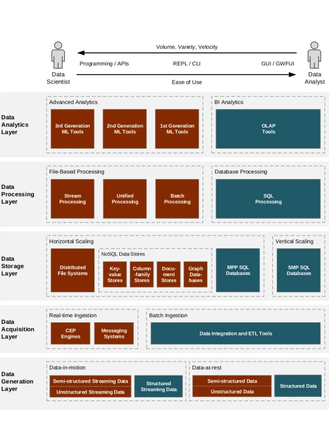
The five layers of the layered reference framework correspond to the process steps of the adaptive Big Data value chain (see Figure 2). As notable differences, the framework handles the technologies corresponding to the data acquisition and preprocessing step from the value chain individually in two separate layers. Layer elements are ordered with increasing volume, variety,

and velocity from right to left. While traditional

BI technologies are indicated in blue (right side), components associated with advanced analytics are colored red (left side). However, the transition between BI and advanced analytics is smooth, as components sometimes belong to both groups, depending on the use case.

While advanced analytics requires input of data scientists [1], traditional BI technologies are usually set up by data analysts without profound mathematical

knowledge [59]. Thus, the former usually requires

good programming skills and knowledge on analytical tools using Application Programming Interfaces (APIs), Read-Eval-Print Loops (REPLs), and Command-Line Interfaces (CLIs), while the latter can often be employed using Graphical User Interfaces (GUIs) or Graphical Workflow User Interfaces (GWFUIs). This corresponds to the easy of use structuring from left to right.

The layered reference framework does not visualize single technologies, but classifies them by their type into different structural elements such asDistributed File SystemsandOLAP tools. As there are lots of tools and projects arranged in each of these elements, there is not a single solution for a given use case [38, p. 41].

Data Generation Data Acquisition and (Pre-) Processing Data Analytics Data Storage

Figure 1: Adaptive Big Data Value Chain (based on [16], [33], and [11])

2.1

Data Generation Layer

The data generation layer deals with different types of data sources. The main differentiating dimensions are variety and velocity. While velocity differentiates between data-in-motion and data-at-rest [28], variety determines among structured, semi-structured, and unstructured data.

Data-in-motion summarizes all data that is constantly generated at low and high velocities, also known under the umbrella term streaming data. It describes events

that need to be analyzed as they happen. Examples

include social media streams (e.g., Twitter APIs such

as Firehose1, Facebook2 or Xing3.), sensor data, and

log files for security access, as well as multimedia streams from music and video platforms and surveillance

cameras. Other examples include high-frequency

financial or transactional structured data streams. The counterpart of data-in-motion is data-at-rest [28]. This term summarizes historically generated data at fixed locations with no velocity. It includes all data that needs to be stored prior to analysis.

The distinction between data-in-motion and data-at-rest influences technology selection. Business use cases usually put requirements on response times and latency

of analysis results. For instance, an earthquake or

tsunami warning system is required to provide warnings in real-time, not on the next business day. Consequently, the velocity of data generation and its required analysis latency have a reasonable impact on the selection of suitable technology.

Notably, more than 95% of all data is unstructured

or semi-structured and thus requires additional

preprocessing [29]. This work also uses the term

1 _{http://www.brightplanet.com/2013/06/}

twitter-firehose-vs-twitter-api-whats-the-difference-and-why-should-you-care/

2 _{See https://developers.facebook.} com/docs/graph-apifor further information.

3 _{Seehttps://dev.xing.com/docs/resources}

multi-structured data as a generalization of

semi-structured and unsemi-structured data. All of these data

can be data-in-motion (streaming data) or data-at-rest,

depending on the use case at hand. The share of

multi-structured data is constantly growing as everyday contents such as video, images, documents, log files, and e-mails contribute to these groups [6]. The resulting data is diverse as it includes unstructured text, logs, scientific data, pictures, voice and video records as well as sometimes metadata [38]. However, currently, structured input data has still a major role in analytical tasks, even with Big Data (e.g., cf. [50]).

2.2

Data Acquisition Layer

The data acquisition layer deals with technologies for an ingestion of data into Big Data infrastructures [38].

The main differentiating dimension is velocity. It

distinguishes between batch and real-time ingestion. Real-time ingestion is sub-divided into messaging systems and Complex Event Processing (CEP) engines, while batch ingestion includes traditional Extract-Transform-Load (ETL) data integration tools. Sample technologies for the different layer elements are given in Table 2.

Batch ingestion has been done for decades in traditional Business Intelligence and Analytics (BI&A)

environments (cf. [36]), is very well researched (cf.

[23]) and is widely understood. Usually, data flows

like ETL, Load-Transform (ELT), or Extract-Transform-Load-Transform (ETLT) are specified (cf.

[38, 19]). Which of these order variations to use is

determined by the use case and its data characteristics

[28]. Most traditional tools such as Microsoft SQL

Server Integration Services (SSIS) and Pentaho Data Integration (PDI) allow integration of both, structured and multi-structured content, between traditional file systems and RDBMSs. Connections to new, distributed types of Big Data storages such as Hadoop Distributed

Data Acquisition Layer Data Generation Layer Data-in-motion Data-at-rest Structured Streaming Data Semi-structured Data Structured Data

Real-time Ingestion Batch Ingestion Data Storage Layer Data Processing Layer Data Analytics Layer

Horizontal Scaling Vertical Scaling

SMP SQL Databases MPP SQL

Databases

NoSQL Data Stores

Distributed

File Systems _value Key-Stores Column -family Stores Docu-ment Stores Graph Data-bases Stream Processing Unified Processing Batch Processing

Advanced Analytics BI Analytics

OLAP Tools

CEP Engines

Messaging

Systems Data Integration and ETL Tools

Database Processing File-Based Processing Data Analyst Data Scientist

Programming / APIs GUI / GWFUI

Ease of Use Volume, Variety, Velocity

REPL / CLI SQL Processing 1st Generation ML Tools 3rd Generation ML Tools 2nd Generation ML Tools Unstructured Data Semi-structured Streaming Data

Unstructured Streaming Data

Table 1: Layered Reference Framework – Data Generation Layer

Layer Element Examples

Structured Data Tabular, transactional, inventory, and financial data

Semi-structured Data XML files, JSON documents, e-mails

Unstructured Data Text, images, videos, and log files

Structured Streaming Data High-frequency transactional and financial data

Semi-structured Streaming Data Sensor and event data, Twitter streams

Unstructured Streaming Data Log files for security, audio, video, and live surveillance

Table 2: Layered Reference Framework – Data Acquisition Layer

Layer Element Exemplary Technologies

Data Integration Tools Apache Sqoop(http://sqoop.apache.org/)

Microsoft SQL Server Integration Services Pentaho Data Integration

Talend Open Studio for Big Data

Messaging Systems Apache Kafka(http://kafka.apache.org/)

CEP Engines Apache Flume(http://flume.apache.org/)

Apache Storm(http://storm.apache.org/)

File System (HDFS)4 _{and HBase}5 _{can be established}

using new technologies such as Apache Sqoop6_.

Real-time ingestion of data-in-motion differs severly from batch-processing and pushes processing and analytics down to the acquisition layer such that the data is essentially processed before it is stored [28]. This is done because it is not reasonable to store all incoming events, due to the velocity of up to millions of events per second and the associated large data volume [13].

Supporting technologies for real-time ingestion

include CEP engines that search streams of data for predefined events and compute results on the fly as they

arrive.7 _{Such systems allow essential operations such as}

aggregation, union, joins, and filtering on input streams to perform predefined analysis, automatic decisions

and actions in real-time. By filtering events prior

to ingestion, only the information needed is assessed, analyzed, and eventually stored [28] [19]. Typical use cases are early warning systems [8], fraud detection (e.g., large withdrawal from bank accounts), mouse clicks on website, security systems, and the assessment of new tweets. In general, this is used when the system must decide immediately whether to disregard an event or perform an action as the situation does not allow to wait for human interaction [28].

4 _{http://hadoop.apache.org/; see also [22].} 5 _{https://hbase.apache.org/}

6 _{https://sqoop.apache.org/docs/1.4.6/} SqoopUserGuide.html

7 _{This can be compared with an ETL pipeline that has near-zero} latency [19].

In between CEP engines and traditional batch-oriented ETL tools are messaging systems. They do not provide functionality for processing of data streams but rather serve as a messaging queue between systems to ensure that no message gets lost. Such tools are oftentimes used to enqueue events and messages from external sources before they are processed by a CEP engine. They furthermore allow communication using a publish-subscribe paradigm between loosely coupled parts of a system [24].

2.3

Data Storage Layer

The data storage layer deals with technologies for persistent data storage in Big Data infrastructures. The main differentiating dimensions are volume and

variety. Variety distinguishes among different types

of storages, namely distributed file systems, Not-Only SQL (NoSQL) data stores, and RDBMSs. These are ordered with increasing data structure flexibility from right to left within the layered reference framework. While structured data is well supported by RDBMSs, multi-structured data requires NoSQL or distributed

file systems. NoSQL data stores are particularly

sub-divided into key-value, document, graph-based and column family stores. The expected overall data volume determines if horizontal or vertical scaling systems are required [55]. In case of horizontal scaling (see [55]) for multi-structured data, the maximum supported data volume is used to order NoSQL and distributed file systems with increasing capabilities from right to left.

Exemplary technologies for different layer elements are given in Table 3. The ones in brackets are not explicitly included in the selection framework introduced later, but will be introduced in future versions.

RDBMSs can be categorized as Symmetric Multi Processing (SMP) RDBMSs and Massively Parallel Processing (MPP) RDBMSs [28] [33]. SMP RDBMSs make use of vertical scaling, while MPP RDBMS scale horizontally (cf. [52]).

MPP RDBMS are best suited for large Data

Warehouse (DWH) applications and in-database

analytics, in particular for Big Data environments, while they still exploit the commonly known and well understood relational data model [28] [33]. This is, among other reasons, because of the horizontal scaling which increases performance and throughput

[55] through inter-node parallelism [10]. Also, they

can be combined with traditional Online Analytical

Processing (OLAP) tools.8_{. However, MPP databases}

typically require their own special purpose hardware [28, p. 16] and need specialized linkage [10] which result in higher costs. Examples for MPP databases are Teradata, Netezza, Greenplum, Vertica and SAP Hana [33] [14]. MPP RDBMS are designed for structured data, not multi-structured data [16, 33]. Nevertheless, MPP RDBMSs are still relevant for Big Data, as long as the workload focusses on structured data.

For multi-structured data, other techniques like

NoSQL data stores and distributed file systems are more promising. The latter usually allow any kind of workloads stored within files [16]. This makes them most suitable for exploratory analysis, which can be used to extract structure from multi-structured data, that can be stored and analyzed using other technologies such as MPP RDBMSs [28]. Distributed file systems allow multiple clients to access files and directories provided on several hosts sharing a computer network. A prominent example for such a system is the HDFS. Key features are automatic data distribution, high availability, fault tolerance, and high throughput access [5]. It allows to dynamically scale up and down while the system

automatically re-distributes the data [33]. Compared

to MPP RDBMSs, HDFS storage is cheap, requires no licensing costs, and runs on commodity hardware.

In between MPP RDBMSs and distributed file systems are NoSQL data stores. They represent a new category of database systems that includes four different types: key-value, document, and column-family stores as well as graph databases [54, p. 122] [48]. Each of them is specialized for specific purposes and workloads (e.g.,

8 _{Microsoft SQL Server Analysis Services (SSAS) can for} instance directly connect to Teradata. See https:// msdn.microsoft.com/en-us/library/ms175608.aspx for further information.

cf. [2]). Therefore, NoSQL gave rise to the polyglot persistence approach, where different data stores are used depending on situation and workload [51]. Features of NoSQL include low latency, low-cost commodity nodes, and the ability to deal with multi-structured data [39]. On the one hand, they allow to easily increase performance linearly with number of nodes. Yet they lack standards and are reported to have bad analytical performance [39].

High performance real-time support for read and write operations can be achieved by using in-memory

storage functionality. The key idea is to eliminate

slower storages on lower levels of the storage hierarchy [31]. In-memory databases load their entire data into memory on startup and use it as their primary storage to achieve permanent higher velocity and lower latency

on read operations [31]. Because of their enhanced

speed, they enable processing of higher data volumes in shorter time such that they are most suitable for data-in-motion scenarios (e.g., streaming data from sensors). In combination with horizontal partitioning, their performance increases almost linearly to the number of nodes. Overall, databases with in-memory capabilities are highly relevant in the context of Big Data as they directly address the volume and velocity dimensions of the original 3 Vs (Volume, Variety, and Velocity) [58].

A survey by KING and MAGOULAS with data

analysts and scientists from 2014 [37] reveals that Structured Query Language (SQL) is used by 42% of the respondents while HDFS is only used by 23%. Similarly, a Jaspersoft survey shows, that most popular storage systems within enterprises are RDBMS (56%), MongoDB (23%), MPP RDBMSs (14%), and HDFS

(12%) [53]. Conclusively, RDBMSs have not been

replaced by other tools. They are still the cornerstone of data analytics, even in the Big Data era.

2.4

Data Processing Layer

This layer includes technologies that are responsible for the execution of data operations such as read, write, and delete, where the main differentiating dimensions

are velocity and variety. Variety determines between

database and file-based processing. While structured

data can be processed using database processing of RDBMSs, multi-structured data is usually stored as files and processed within distributed file systems or NoSQL stores. File-based approaches are particularly sub-divided into batch, unified, and stream processing, depending on the velocity requirement for first results in descending order. Associated processing technologies are abbreviated as Batch Processing Engines (BPEs),

Table 3: Layered Reference Framework – Data Storage Layer

Layer Element Exemplary Technologies

SMP RDBMS Microsoft SQL Server, (MySQL)

MPP RDBMS Greenplum, (Vertica, Teradata)

NoSQL Key-value Store Riak

NoSQL Document Store MongoDB

NoSQL Column-family Stores HBase

NoSQL Graph Databases Neo4J

Distributed File Systems HDFS

Processing Engines (SPEs) respectively. As the data

generation speed must fit the data processing speed for some applications [33], they must be carefully chosen with regard to the use case at hand. Exemplary technologies for different layer elements are given in Table 4.

A distributed processing engine can be seen as an

infrastructure rather than a tool. It is an enabling

technology that can be used or build upon, for instance by analytical tools, which employ large scale machine learning algorithms. Big Data necessitates the use of distributed technologies [8]. New distributed processing technologies constantly emerge [17].

Database processing utilizes functionalities of

underlying databases to perform operations over data within their repositories [22]. Costly data movement is not necessary. Functionalities includes typical SQL

operations such as joins or aggregations (e.g.,Sum) and

groupings [22, p. 356]. Some databases also support enhanced functionalities such as regular expressions [22] or user-defined functions (UDF) [22].

When combined with MPP RDBMSs, database processing is considered even faster and more efficient than file-based in-memory processing with large datasets

[22]. It is therefore a reasonable choice for the

deployment of machine learning algorithms. In contrast, file-based processing cannot be done with off-the-shelf

software [38]. As the data is rarely structured and

diverse, it requires custom coding to derive structure and meaningful insights, as in the approaches described next. Batch processing is used in situations where the entire data is stored prior to analysis [33]. BPEs are capable to handle large amounts of data-at-rest. Algorithms divide data into chunks and process each of them individually on its own machine to generate intermediate results, which are eventually aggregated to a final result. Such execution jobs are predefined by programmers, given to the system, and executed over a longer period of time. They cannot be adjusted while execution is in progress. MapReduce [20] is a representative for BPEs.

Stream processing handles high frequency

data-in-motion and is used in situations where immediate

results are required [17]. Although it is considered

challenging to build a real-time streaming architecture [5], organizations frequently move towards collecting

and processing real-time data [53]. Apache Storm9 _is

a representative for SPEs.

Unified processing aims to combine the advantages of batch and streaming into a single system for processing both data-at-rest and data-in-motion. UPEs provide a single programming model for all purposes and usually employ micro-batches to simulate stream processing. Such systems do not provide real-time but near-real-time processing. While the former seeks to guarantee results within application-specific time constraints, the

latter does not. Unified processing furthermore aims

to provide users with interactive query capabilities and fast answers, even for large amounts of data-at-rest [5]. Thus, engines in this category employ in-memory storage to better support low latency queries and iterative workloads such as machine learning [40]. This is also

denoted as iterative-batch processing [40]. A

well-known representative for UPEs is Apache Spark10.

2.5

Data Analytics Layer

The data analytics layer comprises technologies

responsible for the value generating process of the

adaptive Big Data value chain. Such technologies

uncover hidden patterns and unknown correlations to improve decision making [33] and are a means for

implementing Big Data use cases. Data analytics is

differentiated by two dimensions: the type of data

analytics and the generation of machine learning. The former distinguishes (cf. [57] [56]) technologies by their support for descriptive (cf. [56]), predictive (cf. [57] [56]), and prescriptive (cf. [56]) methods, which are eventually condensed to Business Intelligence (BI) and advanced analytics. BI analytics focuses on descriptive

analytics (e.g., OLAP), while advanced analytics

9 _{http://storm.apache.org} 10_{http://spark.apache.org/}

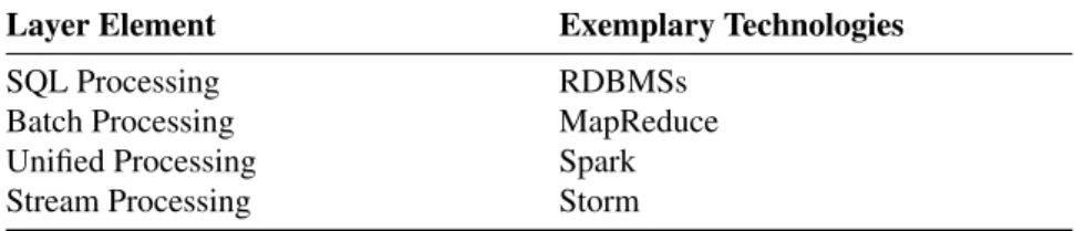
Table 4: Layered Reference Framework – Data Processing Layer

Layer Element Exemplary Technologies

SQL Processing RDBMSs

Batch Processing MapReduce

Unified Processing Spark

Stream Processing Storm

focuses on predictive and prescriptive analytics [32]. Advanced predictive or prescriptive analyses typically employ machine learning (cf. [57] [42] [22]). Machine

learning methods, among others, include11_{classification}

(cf. [26, 34]), regression (cf. [46]), topic modeling (cf. [15] [22]), time series analysis (cf. [22]), cluster analysis (cf. [22], [18, 26]), association rules (cf. [46] [22]),

collaborative filtering (cf. [4, 34]), and dimensional

reduction (cf. [49, 60]). Advanced analytics can be further described by a maturity model proposed by AGNEESWARAN [3], which distinguishes analytical tools into three generations of machine learning as follows:

1st Generation Machine Learning (1GML)requires the data workload to fit into memory of a single

machine. Such tools are restricted to vertical

scaling (cf. Section 2.3), which is a drawback when

considering Big Data. Tools in this group were

usually developed before Hadoop and are referred

to astraditional analytical tools. Usually, vendors

try to enhance or re-engineer their products in a way that allows the usage of Big Data. Mostly, connectors are added that allow read and write operations to HDFS while the analysis is still performed within the tool. Hence data is exported from storage, analyzed, and later re-imported12_. 2nd Generation Machine Learning (2GML)

enhances 1GML with capabilities for distributed

processing across Hadoop clusters. In contrast

to 1GML, data remains at its location while the code execution is divided and processed on each required data node in parallel13_{. Tools in this class}

are denoted asover Hadoop[3]. Many algorithms

do not translate easily into MapReduce [40]. While non-iterative algorithms can be translated into efficiently performing series of MapReduce operations, iterative algorithms such as machine learning cannot. Thus, the expected performance for such workloads is poor.

11_{http://machinelearningmastery.} com/a-tour-of-machine-learning-algorithms/

12_{This is referred to asdata-to-code.} 13_{This is referred to ascode-to-data.}

3rd Generation Machine Learning (3GML)

enhances 2GML with capabilities to efficiently

perform distributed processing of iterative

algorithms. This class is referred to as beyond

Hadoop. Associated tools such as Spark use more advanced distributed processing methods or in-database execution to cope with some of the disadvantages that come with MapReduce.

Sample technologies for different layer elements and machine learning generations are given in Table 514_.

Usually, tools evolve over time due to re-engineering

efforts by vendors. For instance, Mahout just

recently evolved from 2GML to 3GML as it now

supports processing on Spark, Flink and H20 along

with MapReduce. As these engines support efficient

execution of iterative machine learning algorithms, Mahout is classified into two layer elements.

The distinction between BI and advanced analytics

is supported by a study of KING and MAGOULAS

[37]. According to them, traditional data analysts use commercial tools such as Excel, Microsoft SQL Server, and Tableau for explanatory BI for descriptive analytics.

On the other hand data scientists (cf. [59]) utilize

open source tools like R, Apache Hadoop, and scalable

machine learning such as Apache Mahout15_.

BI analytics is about dicing, slicing, drill-up,

drill-down, and drill-through operations over cleaned historical data using a predefined multidimensional model [22] [13]. This can be done using server-based OLAP Engines such as Microsoft SSAS and Pentaho

Mondrian16_{. For small amounts, simple off-the-shelf}

software like Excel can be sufficient.

Big Data analytical solutions can be differentiated as offline and online analytics [16] as well as combined

approaches (cf. [55]). Online analytics is used for

real-time environments that require low latency for results, especially with data-in-motion. Offline analytics

14_{All tools are classified without extensions. Extensions could allow} to tools be classified in a higher tier, e.g., Microsoft R (https:// mran.microsoft.com/open/, formerly Revolution R), which enables distributed execution over Hadoop clusters

15_{http://mahout.apache.org/}

16_{See http://community.pentaho.com/projects/} mondrian/.

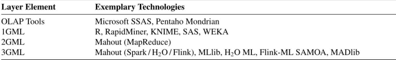
Table 5: Layered Reference Framework – Data Analytics Layer Layer Element Exemplary Technologies

OLAP Tools Microsoft SSAS, Pentaho Mondrian

1GML R, RapidMiner, KNIME, SAS, WEKA

2GML Mahout (MapReduce)

3GML Mahout (Spark / H2O / Flink), MLlib, H2O ML, Flink-ML SAMOA, MADlib

usually employs batched processing for ingestion, transformation, and analytics.

While latency (cf. [40]) is the most important

factor for online-analytics, throughput is essential

for offline-analytics [12]. Latency highly depends

on the technologies for processing and storage on the corresponding layers of the layered reference

framework. While online-analytical systems usually

operate on SMP, MPP, and NoSQL databases using in-database, stream, or unified processing, offline-analytical tools usually employ distributed file systems in combination with batched processing [28].

A survey among data analysts and data scientists from 2014 [37] reveals that in-database analytics with SQL is used by 71% of the respondents, while the next high ranked tool, R, is only used by 43%. Only 7% of the respondents use Mahout. NoSQL and Hadoop may have solved the storage problem for large amounts of raw data, but still seem unable to sufficiently fulfill needs of business users with regard to data analytics.

3

T

S.T.A.D.T. S

F

This section introduces our Strategy, Time, Analytics,

Data, and Technology (S.T.A.D.T.) Selection

Framework (abbreviated as SSF), which aims to guide technology selection in the Big Data era. It seeks to find a set of valid solutions for given Big Data use cases. SSF is based on the layered reference framework presented in Section 2 and consists of two parts: a business and a selection process. Figure 3 provides an overview of the framework.

The business process is partly based on Marr’s

SMART Model [43], which can be used as a guideline on how to evolve towards a Big Data driven smart

business. However, the S.T.A.D.T.SSF as presented

here is fundamentally different, except for the general

idea of the first two process steps of strategy and

measures (here: data). The SSF aims at selection of technology, not at business transformation, and hence

reinterprets and renames the process steps by MARR

to reflect this change (Strategy, Time, Analytics, Data,

and Technology). In this way, it is similar to the

GOBIAmethod of [27], which also combines a reference

architecture with a development process. Notably, the process of technology selection could be extracted from the SSF and be seamlessly embedded as final step in the

GOBIA method development process (GOBIA.DEV, cf.

[27]).

The business process of the Strategy, Time,

Analytics, Data, and Technology (S.T.A.D.T.) Selection Framework (SSF) serves as a roadmap for companies who want to select appropriate technologies for their Big Data use cases at hand. It starts with the overall strategy, i.e., business objectives to be achieved [43]. Depending on the strategy, measures of input data, suitable analytics and required response times are derived and used to select suitable classes of storage systems, analytical tools, and processing engines respectively. Finally, a suitable technology mix is selected that corresponds to the input use case.

All steps of the SSF’s business process have

implications on technology selection. They filter the

layered reference framework and thereby narrow the

search space for valid solutions. First, the overall

strategy is used to select relevant layers. Secondly,data

measures, analytical requirements, and response times

determine relevant layer elements. Finally, the remaining technologies are filtered by their interdependencies (e.g., compatibilities), individual properties as well as user preferences to derive the final solution space.

There is no single decision tree that determines the right technology mix with respect to all conceivable circumstances [51]. Thus, our SSF aims to find the set of best suited technologies in each selection step. It does not seek a complete list of possible technology sets for a use case. As the great potential for Big Data arises when different technologies are used in concert, it attempts to recommend at least one tool on every required layer for further investigation.

The remainder of this section follows the structure

of the SSF business process. It starts with strategy

(cf. Section 3.1), defines requirements on (response)

times (cf. Section 3.2), decides on analytics

(cf. Section 3.3), then continues with data (measures) (cf. Section 3.4), and finishes with selection of suitable

technologies (cf. Section 3.5). Each process step is

T

A

D

T

S

Figure 3: The S.T.A.D.T. Selection Framework

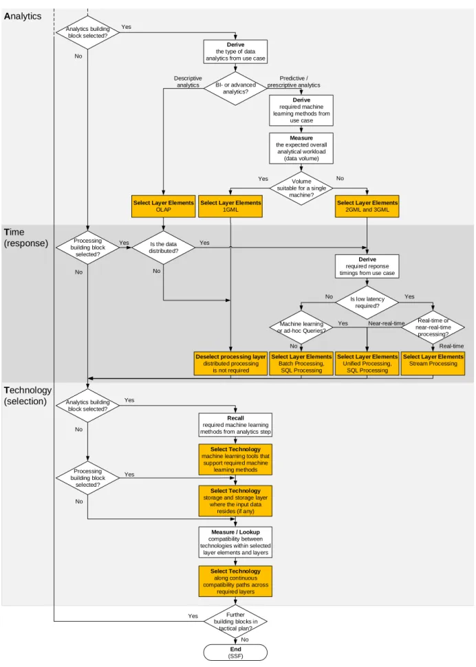
resulting implications on technology selection. The

complete SSF process is illustrated in 5 and 6, in the form of flow charts.

3.1

Strategy

This section deals with Big Data strategies and their transformation into executable tactical plans. It describes different building blocks and associates each with required layers and steps of the SSF’s business process. While the development of a specific Big Data strategy is out of scope, this section still provides a brief strategy guideline as well as a description of organizational requirements and impacts.

Overall, strategy is essential and drives the selection of technology [27]. Big Data initiatives need to be aligned with the overall business strategy [28]. Prior to analysis of Big Data, it is essential to derive relevant and business

related questions that need to be answered17 _{(see also}

[43] [21] [28]).

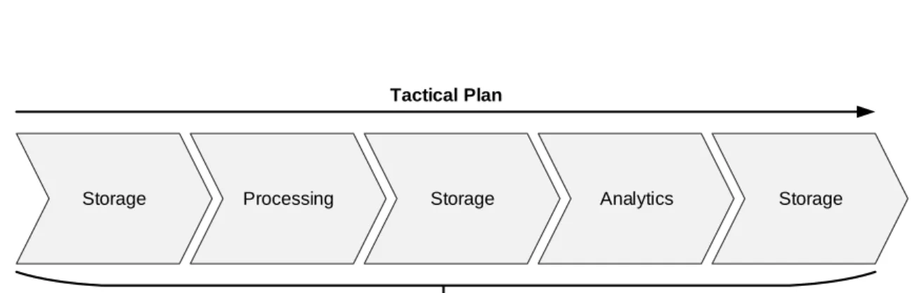
Once a strategy has been settled and a business relevant question has been derived, it can be translated into an executable tactical plan. Initial building blocks are storage, processing, and analytics, because they represent categories for typical Big Data use cases respectively Big Data products used in these use cases. These building blocks can be arranged in any sequence of arbitrary length to solve a business relevant question. Each block starts a new iteration of the SSF process and covers a unique functionality. Storage for instance

17_{http://practicalanalytics.} co/2015/05/25/big-data-analytics-use-cases/

acquires and stores data from any sources. It makes sure that the data is stored in an appropriate data store that fits the data at hand. Processing transforms data from one state to another within the data source it resides, e.g., from multi-structured data to structured data. Finally, analytics performs machine learning algorithms to create additional value. Figure 4 provides an sample tactical plan.

Firstly, a storage building block acquires for instance multi-structured data from an external source and stores it in a suitable storage system within the infrastructure,

e.g., HDFS. Secondly, a processing building block

transforms the data into a structured format, while it

remains within HDFS. The third iteration takes the

processed data from HDFS as source and stores it in the most suitable storage system of the infrastructure, e.g., into a RDBMS. The subsequent analytics building block performs machine learning algorithms on the data stored in the RDBMS. Such blocks may also employ a distributed processing engine to fulfill their task. Finally, the storage building block seeks the best suited system to store the analytical outcome.

Each type of building block seeks technologies at different layers of the layered reference framework (cf. Section 2). The assignment of building blocks to layers is given in Table 6.

Storage for instance seeks compatible technologies on two layers: the data acquisition layer and the data storage layer. Analytics searches for compatible technologies on the data processing and the data analytics layer while considering a specific storage system as input source. This is indicated by using parentheses. Processing can

Storage Processing Storage Analytics

Building Blocks Tactical Plan

Storage

Figure 4: Building Blocks for Tactical Plans: Storage, Processing and Analytics

Table 6: Building Blocks – Layer Assignments Layer Storage Processing Analytics

Data Analytics _{6 6 4}

Data Processing _{6 4 4}

Data Storage 4 (4) (4)

Data Acquisition 4 6 6

be described analogously. Note that the data generation layer is not listed in Table 6 as it does not contain technologies but data characteristics, which are used for filtering layer elements in Section 3.4.

Different types of building blocks also require other SSF process steps. Their mappings are given in Table 7. For each building block, the associated steps need to be executed in their corresponding top-down order to receive a suitable technology mix. This is automatically taken care of by the process flow charts in figures 5 and 6.

Storage building blocks for instance rely solely on the data and technology steps, while analytics building blocks require the latter three steps of analytics, time, and technology. Required steps for processing building blocks can be derived analogously.

The decomposition of a use case into sequences of storage, processing, and analytics has at least two

advantages. Firstly, it narrows the search space for

each block, which makes especially large and extensive

Big Data use cases more tangible. Secondly, the

decomposition only requires to understand the purpose of each building block and can be carried out by business staff without extensive IT expertise.

However, decomposition may lead to an over-optimizing of solutions as building blocks are handled in isolation. The result may be many “locally optimal” pieces of technology, which each require specially

Table 7: Building Blocks – Process Step Assignments SSF Process Step Storage Processing Analytics

Measures _{4 6 6}

Analytics _{6 6 4}

Response 6 4 4

Technology 4 4 4

trained staff and integration. Trade-offs have to be

made to select few, yet manageable ones. But this

consideration is out of scope of this work and not yet covered by the SSF.

3.2

Time

This section handles the selection of best-suited layer elements with regard to processing in distributed environments. Hence it is only needed in cases where the underlying data is stored in distributed storage systems

[48]. In such cases, the selection depends on the

assessment of required response times to be derived from

the use case. If the data is not stored in distributed

storage systems, then distributed processing is also not required. In such cases, the whole processing layer is deselected and not used in the final technology selection

step (cf. Section 3.5). The process is illustrated in

Figure 6 and elaborated upon in subsequent paragraphs. In case of distributed data, users need to specify their requirements for latency (cf. Section 2.5). Essentially, they need to determine if the latency of a result is a

fundamental measure for their use case at hand. If

so, the use case needs to be assessed to determine if specific time constraints are prescribed that must be guaranteed. In cases where real-time results are needed (i.e., where short response times must be guaranteed), SSF selects stream processing as the most suitable

layer element. In cases where near-real-time results are sufficient and small random time gaps (e.g., a few seconds) between data arrivals and processing results are acceptable, SSF selects SQL [55] and unified processing. The latter uses micro-batches to simulate streaming (cf. Section 2.5). This comes with more latency but also with less complexity compared to stream processing. Unified processing furthermore unifies the programming model for batch and streaming, which makes it a more

universal tool. As such, it should be preferred over

stream processing where possible [40].

If low latency results are not fundamental for a given use case, it is not recommended to use SPEs due to their complexity [40]. In such situations, batch or iterative-batch processing are more suitable (cf. Section 2.4). Such engines come with higher latency but allow high throughput [44]. The choice between the two depends

on the need for iterations. Ad-hoc queries and most

machine learning algorithms are iterative in nature [55]. Thus, SSF selects unified and SQL processing in case of their presence. In all other cases, the usage of batch processing is sufficient, such that the corresponding layer element is selected.

3.3

Analytics

This section prepares the selection of suitable machine learning tools. It aims to select best suited layer elements on the corresponding layer of the layered reference framework. The selection depends on three factors: the required type of analytics, the expected data volume and the required machine learning methods (cf. Section 2.5). The process is illustrated in Figure 6 and discussed in the following paragraphs.

The first decision determines between BI and

advanced analytics (cf. Section 2.5). The former

represents descriptive methods while the latter

emphasizes predictive and prescriptive analytics. In

case of descriptive analytics, traditional BI technologies such as OLAP tools are naturally supportive and thus selected. In case of predictive or prescriptive analytics, the required machine learning methods need to be derived to select appropriate tools in the later technology selection step of the SSF [55]. For instance, if a use case aims to provide recommendations, then it usually employs collaborative filtering. Clustering can be used if a use case needs to find similar entities, e.g., groups of customers.

The expected data volume determines the minimum required generation of machine learning for a given task (cf. Section 2.5). While 1GML tools are sufficient for data workloads that can be analyzed on a single machine, 2GML or 3GML are required in situations that determine horizontal scaling (cf. Section 2.5). The latter two need

distributed processing engines while 1GML does not. Such tools process data in local memory and just connect to arbitrary storage systems for read / write operations. If a task can be analyzed on a single machine, then that is the recommended solution. 1GML tools are easier to handle, more mature, and more extensive in their machine learning capabilities than horizontally scaling

tools [40]. So, 2GML and 3GML technologies are

only recommended in situations that require distributed

processing due to high volumes. The actual choice

between the two is implicitly further refined in the

time-step of the SSF by selection of processing types

(cf. Section 3.2).

There is a variety of different tools for advanced analytics available on the market. Because of their large numbers, it is not reasonable to handle them in this work simultaneously. Instead, a representative subset

is selected and evaluated. KDNUGGETS18 considers

itself as one of the top web resources for analytical software and conducts a poll about their usage every

year. The results for 2015 are based on 2,800 votes

by users of the data mining community, who have

chosen from a record of 93 different predefined tools

[47]. With some adjustments, these results can serve as the foundation for tool selection in the work at hand. Firstly, formal languages like SQL, Python, Perl,

Pig, and Lisp are removed from the list. Secondly,

all 1GML tools other than the top 3 with regard

to usage are removed. The same holds for Big

Data processing engines and analytical tools without capabilities for advanced analytics (i.e., predictive or

prescriptive methods) (cf. Section 2). Furthermore,

spreadsheet tools with a focus on office users like Excel are excluded. Finally, the list is extended by promising findings during literature research and interviews for this work. Examples for such include MADlib, Flink ML and SAMOA. Additionally, Microsoft SSAS is included as a representative for OLAP engines.

The gap between 1GML and 2GML / 3GML tools with regard to their usage suggests that most analytical use cases are still solved with traditional tools, even in the Big Data era.

3.4

Data

This section deals with measurements of data

characteristics, which are used to select layer elements on the data acquisition and the data storage layer. The overall goal is to find layer elements that are best suited for the data at hand. For this, a proper understanding of data characteristics is key to success [30].

A starting point are the well-known 3 Vs of Big

Data [22]: volume, variety, and velocity. While velocity distinguishes between in-motion and data-at-rest [55], variety distinguishes between structured and multi-structured data [22] (see also Section 2.1). Furthermore, the volume dimension determines how

much scalability is needed. It distinguishes between

horizontal and vertical scaling (cf. Section 2.3) [40]. As the desired infrastructure must be scalable for the future, all decisions on data characteristics have to support the current and the future dataset [16]. Thus, not the current state needs to be measured, but the expected one.

The assessment of the 3 Vs follows a three-step process, as illustrated in Figure 5. Firstly, the velocity

dimension is inspected. It determines between

data-in-motion and data-at-rest. Both require fundamentally different technologies and methods for data acquisition

(cf. Section 2.2). While data-in-motion leads to the

selection of CEP engines and messaging systems [44], data-at-rest selects the layer element for traditional data

integration tools. The respective flow chart part in

Figure 5 highlights all process steps for selections with orange color.

Secondly, the volume dimension needs to be

inspected. It determines whether a Big Data platform is required or whether the data can be processed on a single machine [55]. Big Data technologies should not

be used if there is no need to do so [5] [51]. It is

a magnitude easier to solve problems with traditional SQL based systems or by using script-based processing of multi-structured data on the local file system of a

single machine [40]. These tools are less complex

[51], more mature, widely understood, and broadly

available. In a nutshell, if the data volume allows

storage and processing on a single machine, then that

is the recommended solution. In this case, SSF

selects RDBMSs and recommends to use local non-distributed file systems in combination with scripts for

data transformation. Notably, through the years, a

typical server’s capabilities have continuously increased, making a volume-based decision between a distributed

system and a single machine time-dependent. For

instance, single machine servers can easily possess

several TB of main memory nowadays19,20, whereas it

was only hundred or a few hundred GB less than 10 years ago21.

In cases where the overall expected volume exceeds a single machine’s capacity with regard to storage, CPU, or memory [5], the variety dimension needs to be

19_{http://www.alphr.com/news/enterprise/387196/} intel-xeon-e7-v2-servers-support-6tb-of-ram 20_{https://www.theregister.co.uk/2017/05/16/}

aws ram cram/

21_{http://www.pcworld.com/article/161822/} article.html

inspected to select a best suited storage system. While structured data is well-suited for MPP RDBMSs, multi-structured data requires NoSQL stores or distributed file systems. The selection for multi-structured data can be further refined by assessing the expected number and

size of files [51]. For small numbers of large files,

it is suggested to use distributed file systems. For

large numbers of small files, the recommendation is to

use NoSQL stores. MARZ [44] explains that Hadoop

can be a magnitude slower for processing of many small files compared to few big files, although both scenarios have the same overall volume. Reasons for this include high latencies for individual record lookup in HDFS [10]. The framework therefore suggests to select distributed file systems for large files and NoSQL stores for large amounts of small files in accordance with the mentioned authors. However, there are newer distributed file systems with in-memory capabilities for random and fast data access such as Alluxio22_{. For such systems, the}

distinction for number and size of files is less important. If they win recognition, they possibly form a new class of storage systems in the layered reference framework for further distinction. However, this is not yet included in its current version.

The choices for layer elements are derived from interviews [41] and from a comprehensive literature

review. BEGOLI and HOREY [7] for instance provide

some principles for good Big Data architectures. The authors especially give advice on the influence of data

variety on technology selection. They suggest to

use Hadoop for unstructured data, MPP RDBMSs for structured data, and NoSQL stores for semi-structured

data. Similarly, FERGUSON [28] suggests to align

data characteristics with storage and recommends to use MPP RDBMSs for complex analysis of structured data and Hadoop for multi-structured data, especially for storage and processing tasks of archive data. He also discusses the differences between data-at-rest and data-in-motion and their relation to CEP engines, stream

and batch processing. CHAN [10] contributes to the

discussion and argues about the impact of velocity

on technology selection. The author introduces an

integrated conceptual architecture for stream and batch

processing. Finally, MARZ [44] suggests the Lambda

Architecture, which unifies processing of data-at-rest and data-in-motion on a conceptual level.

3.5

Technology

This section handles the final step of the SSF business process, which eventually selects a suitable technology

mix. The selection follows a three-step process as

illustrated in the lower part of Figure 6. Firstly, suitable machine learning tools are selected in cases where

analytics is required. Secondly, the storage system

that holds the input data is selected if the current SSF iteration handles an analytics or processing building block. Finally, interdependencies are inspected to find compatible technology mixes between required layers of the layered reference framework. The results can be further refined by investigation of technology-specific characteristics. Each process step is described in the following paragraphs.

If the current SSF iteration handles a building block for analytics, suitable analytical tools must

be selected. Recall the assessment for machine

learning methods performed in the analytics-step

(cf. Section 3.3). A suitable tool must support the

identified required methods. For proper selection,

Table 8 and Table 9 provide mappings between analytical tools and supported machine learning methods. The SSF process requires all technologies that enable the required methods of the use case to be selected for the later compatibility check.

Note that all assessed 1GML tools support any of

the machine learning methods. As most Big Data

analytical tools offer less functionality compared to solutions that operate in-memory on a single machine, Big Data technologies are less promising for small data [40], which is another indication that they should only be used when certainly needed (cf. Section 3.3).

The mappings in Tables 8 and 9 are based on the

work by LANDSET et al. [40] and RICHTER et al.

[49] who assess analytical tools with regard to machine learning support. This work enriches their findings with additional tools and methods. It furthermore refines their results with information collected from the individual websites and documentations of the tools.

For simplicity, SSF only uses machine learning methods for mappings. However, each of these methods may include several different specific algorithms that are

suitable to fulfill the task. For instance, classification

can be performed with decision trees, linear and logistic regression, Na¨ıve Bayes, Support Vector Machines (SVMs), gradient boosted trees, random forests, adaptive model rules, and generalized linear models [40]. The framework indicates a tool’s support for a machine learning method if one of the enabling algorithms is

included. A more comprehensive list of available

machine learning algorithms as well as their coverage by processing engines is given by the formerly mentioned authors [40] [49]. If needed, SSF can easily be extended with specific algorithms. However, this is out of scope of the work at hand.

The next process step requires to select the input

storage system where the data is located. This is

mandatory for processing and optional for analytical building blocks. While the former always performs on data within the local infrastructure, analytical tasks can also be executed on a data stream without prior storage. This is also explained with the adaptive Big Data value chain in Section 2. If the data to be analyzed is located within the local infrastructure, a specific storage system needs to be selected, thus given as input. In case the data is not stored prior to analysis, the storage layer can be omitted for the subsequent compatibility check.

4

A

A

S

This section examines an application scenario for SSF and thereby demonstrates the technology selection, which is based on continuous paths through the layered reference model and technology capability mappings. The application scenario is first introduced. It features a retailer with an existing traditional data warehouse that has been created based on traditional requirements. These prerequisites are used to infuse the SSF process

to find a suitable technology mix. This section

shows which technological choices SSF suggests in the context of current technologies, and if and to which extend they deviate from the existing choices. Finally, the application scenario is revisited with a new requirement to determine required changes to the underlying technologies to remain compliant with requirements.

4.1

ShopMart

Scenario Characteristics

The usage of a traditional data warehouse with traditional requirements is illustrated using fictitious

German retailer ShopMart. Although the scenario

and its assumptions are fictitious, they represent

common elements in warehouse architectures and related requirements (e.g., reporting or OLAP), which have evolved over time in both research and practice. Thus, the application scenario presented could be applicable to other traditional setups that rely on similar technologies.

The long term goal of ShopMart is to become the

most profitable retailer in the low price segment in Germany with the highest profit margin. The product

selection offered by ShopMart appeals to a broad

customer base (i.e., not too expensive). To achieve

these long term goals, strict cost control mechanisms are employed. This strategy is implemented in its data warehouse with two analytical tools that are represented

as tactical plans in SSF. We outlineShopMart’sgoals and

requirements next; subsequently, the current warehouse implementation is described. With this, the necessary information for the SSF process can be derived (rather

Strategy Analytics Data Select Layers depending on building block Start (SSF) Storage building block selected? Measure

the expected overall data volume

Select Layer Elements

SMP SQL Databases, (and use a local

filesystem)

Measure

data variety Volume

suitable for a single machine?

Structured or multi-structured

data?

Select Layer Elements

NoSQL Data Stores

Select Layer Elements

MPP SQL Databases Data-in-motion

or data-at-rest?

Measure

data velocity

Select Layer Elements

CEP Engines, Messaging Systems

Select Layer Elements

Data Integration Tools Data-at-rest Data-in-motion Yes No Structured Multi-Structured Number and size of input files?

Small amount of large files Large amount

of small files

Select Layer Elements

Distributed File Systems

Derive

tactical plan from strategy

Select

next building block

Analytics building block selected?

Yes No

Time (response) Analytics

Measure

the expected overall analytical workload

(data volume)

Volume suitable for a single

machine?

Select Layer Elements

1GML BI- or advanced

analytics?

Select Layer Elements

OLAP

Select Layer Elements

2GML and 3GML Descriptive analytics Predictive / prescriptive analytics Yes No Derive

the type of data analytics from use case Analytics building

block selected? Yes

Derive

required reponse timings from use case

Is low latency required?

Select Layer Elements

Stream Processing

Select Layer Elements

Unified Processing, SQL Processing

Select Layer Elements

Batch Processing, SQL Processing Machine learning or ad-hoc Queries? Real-time or near-real-time processing? Is the data distributed?

Deselect processing layer

distributed processing is not required Yes No Yes Near-real-time No Real-time Processing building block selected? No Yes Yes No Technology (selection) Select Technology

machine learning tools that support required machine

learning methods Analytics building block selected? Yes No End (SSF) Measure / Lookup compatibility between technologies within selected

layer elements and layers

Select Technology

along continuous compatibility paths across

required layers

Recall

required machine learning methods from analytics step

Select Technology

storage and storage layer where the input data

resides (if any) Processing building block selected? No Yes Further building blocks in tactical plan? Yes No No Derive required machine learning methods from

use case

Table 8: Supported Machine Learning Methods for 1 GML and OLAP Tools (based on [35])

ML Method RapidMiner KNIME R Microsoft SSAS

Regression 4 4 4 4 Time Series 4 4 4 4 Classification 4 4 4 4 Topic Modeling 4 4 4 6 Cluster Analysis 4 4 4 4 Association Rules _{4 4 4 4} Collaborative Filtering _{4 4 4 6} Dimensional Reduction _{4 4 4 6} ML Generation 1GML 1GML 1GML OLAP

Table 9: Supported Machine Learning Methods for 2/3 GML Tools (based on [40] and [49])

ML Method Mahout (MR) Mahout (Spark) Mahout (H2O/Fl) H2O ML Flink ML

MLlib MADlib SAMOA

Regression _{6 6 6 4 4 4 4 4} Time Series _{6 6 6 4 6 6 4 6} Classification _{4 4 6 4 4 4 4 4} Topic Modeling _{4 4 6 6 6 4 4 6} Cluster Analysis _{4 6 6 4 6 4 4 4} Association Rules _{4 6 6 6 6 4 4 4} Collaborative Filtering _{4 4 6 6 4 4 6 6} Dimensional Reduction 4 4 4 4 6 4 4 6 ML Generation 2GML 3GML 3GML 3GML 3GML 3GML 3GML 3GML

abstract tactical plans and, based on these, data, time, analytics process part information).

1. ShopMart points out profit and cost as Key Performance Indicator (KPI) for each subsidiary,

each product, and the combination of the

aforementioned. These are used for daily and

quarterly reports. To this end, ShopMart has

an Enterprise Resource Planning (ERP) system, which collects all transactions (e.g., a customer

buying a product) from the subsidiaries. The

cash registers push their data either in real-time

or asynchronously to the ERP system. From

there, the data warehouse receives the data via ETL processes, which perform data cleaning and transformation procedures to generate materialized views that prepare the data for report generation. 2. ShopMart monitors and analyses current and

historical prices of its various suppliers to select the most cost-efficient supplier for short-term and

long-term contracts. The response time requirements

are stated as “as fast as possible” so that new orders can be placed exactly when the time is right.

The available warehouse technology allows for a response of one day (daily ETL with analytics in

the warehouse) when ShopMart built it. To this

end, ShopMart has various systems in place to

capture current prices. For instance, wholesaler

B2B online shops are scraped regularly to acquire prices for products purchased via wholesales. The captured data is loaded via an ETL process and the placed in the data warehouse for enhanced

analytics. ShopMartcurrently employs time-series

analysis to forecast price trends for its products. The results are saved in materialized views, which are refreshed daily, and supplied to a tool that can access these data via SQL.

These requirements are used to derive two more abstract tactical plans as proposed by SSF (see Figure 7

and Figure 8). These do not refer to specific

technologies, only to the requirements at hand. That way, the technology selection can be done with SSF, after it is introduced in the following section.

(1.1) Storage Acquire and store

facts (sales and purchases) and dimensions (e.g., products) (1.2) Analytics Compose aggregate revenue

and cost KPIs per subsidiary and

product

Figure 7: ShopMartTactical Plan for Profit and Cost KPI Goal (1)

4.2

Technology Selection Approach

Generally, once relevant layers, layer elements and perhaps input data sources have been determined with the SSF process, a suitable technology mix

can be selected (cf. Figure 6). However, it is

necessary that those technologies, which are on adjacent layers in the layered reference model, are compatible

to each other. A continuous path of compatible

technologies along the various layers ensures that a

valid technology mix is proposed. The selection

process checks for compatibilities between candidate technologies within selected layer elements and searches for continuous compatibility paths from the topmost to the lowest selected layer of the layered reference model. Conclusively, every continuous path is a valid solution. Figure 9 provides a scenario that represents an analytical building block with persistent input storage.

In this example, previous process steps have already selected best suited layer elements. Unselected layers and layer elements are faded out and not considered

for the final result. The sample use case requires

machine learning method {1} and data storage {7},

which have been provided as input in the corresponding steps of the SSF process. With this preselection, valid solutions include the sets{1, 2, 4, 7} and{1, 2, 5, 7}as both represent a continuous path from the topmost to the lowest selected layer. The candidate solution{1, 3, 6, 7}

is interrupted, as the analytical tool named{3}does to

support the required machine learning method. Thus it is not a valid solution.

This concept of technology selection requires

compatibility mappings between technologies at

adjacent layers. One example for such is given in

Table 10. It provides mappings for analytical tools and

distributed processing engines. SAMOA for instance

can be employed in combination with Storm or Flink, while MLlib only supports Spark.

The general idea for mappings is based on LANDSET

et al. [40] who also provide a graph-based compatibility mapping between processing engines, machine learning

methods, and analytical tools. This work extends their idea to other layers such as storage and data acquisition to provide a more comprehensive mapping, which can be used for diverse and more customized technology selections.

Valid sets of technologies can be further refined with user preferences and technology specific individual

properties. Storage systems can for instance be

filtered with regard to their preference for consistency, availability and partition tolerance as proposed by the

CAP theorem [9]. In case of distributed systems,

partition tolerance is mandatory [48]. Thus, users can decide between consistency and availability for their use case at hand and filter results accordingly.

4.3

ShopMart

Technology Selection

Applying the SSF technology selection approach to the

ShopMartscenario at hand yields the following results.

Tactical plan for profit and cost KPI goal (1) (1.1) Storage. Storage building blocks work with

storage and acquisition layers (cf. Section 3).

The only input storage here is an operational ERP system out of scope of the analytical system. To decide for layer elements, data velocity, overall volume, and variety need to be clarified upon.

ShopMart uses a traditional ERP solution (SAP ERP), which uses a structured data format. Data Integration Tools are a suitable choice for data acquisition, considering dealing with data-at-rest. For ShopMart the size of an ERP currently fits

inside a single server machine, therefore anSMP

SQL databaseis selected for storage.

As for Oracle and SAP ERP products, for instance, accessing their relational SQL databases to extract

data is considered possible, albeit challenging23.

Furthermore, specialized APIs and connectors can be used to access ERP systems like SAP ERP (e.g., Oracle Business Warehouse offers a connector for

SAP24_{). Some ETL tools also offer SAP connectors}

(e.g., Pentaho Data Integration25_).

(1.2) Analytics. For this case, an analytics building

block is selected. To select it, one must decide

between BI and advanced analytics. Standard

reporting with KPIs is a typical BI analytics task. Therefore, OLAP is selected. Besides dedicated OLAP engines, some data warehouses can be SMP

23_{https://www.quora.} com/Can-I-access-SAP-Oracle-and-most-of-the-ERP-by-SQL

24_{http://docs.oracle.com/cd/E11882 01/owb.112/} e10582/sap integrate.htm#WBDOD30500

25_{http://wiki.pentaho.com/display/EAI/} Connecting+with+SAP+Systems