OBSERVATIONS OF MISOVORTICES WITHIN THE 7 JANUARY 2014 LONG LAKE-AXIS-PARALLEL LAKE-EFFECT SNOW BAND DURING THE ONTARIO
WINTER LAKE-EFFECT SYSTEMS PROJECT
BY
JAKE PATRICK MULHOLLAND
THESIS
Submitted in partial fulfillment of the requirements for the degree of Master of Science in Atmospheric Sciences
in the Graduate College of the
University of Illinois at Urbana-Champaign, 2016
Urbana, Illinois
Advisers:
Professor Robert M. Rauber
ii Abstract
Recent lake-effect snow field projects in the Eastern Great Lakes region [e.g., the Long Lake-Axis-Parallel (LLAP; 2010-2011) Project and the Ontario Winter Lake-effect Systems (OWLeS; 2013-2014) Project] have revealed the presence of misovortices with diameters between 40 and 4000 m within LLAP bands in the vicinity of Lake Ontario. These misovortices usually develop along convergence boundaries associated with cyclonic horizontal shear zones that likely originate from solenoidally-forced secondary circulations within these warm-core bands. In most cases, the shear zone is co-located with a sharp horizontal gradient in radar reflectivity, which corresponds to the region of maximum vertical velocities. One particular band from the OWLeS Project, in which an abundance of misovortices developed, occurred on 7 January 2014.
Steiger et al. (2013) postulated that the release of horizontal shearing instability (HSI) was the main mechanism for misovortexgenesis in two LLAP bands analyzed during the LLAP Project. With data from only a single mobile Doppler radar available, however, this hypothesis was not testable. In the present study, three-dimensional dual-Doppler (DD) wind syntheses reveal that two separate criteria for HSI are met along the low-level horizontal shear zone within this band. This strongly suggests that HSI was the likely cause of the misovortices within this band. Furthermore, the lack of anticyclonic-cyclonic vortex couplets throughout the event reveal that tilting of horizontal vorticity into the vertical is likely of less importance compared to the release of HSI and subsequent vortex strengthening via stretching of low-level vertical vorticity. This vortex stretching is maximized along the low-level convergence zone, where vertical velocities (generally between 1 - 3 m s-1) are greatest owing to the solenoidally-forced transverse secondary circulation of the band.
iii
A high-resolution Weather Research and Forecasting (WRF) simulation was conducted for this case study. The 333-m horizontal resolution domain depicts the presence of misovortices along the cyclonic horizontal shear zone within the band. The simulation also reveals that a linear vortex sheet originates in the vicinity of Lake Huron and Georgian Bay, and extends over Lake Ontario. This vortex sheet breaks into discrete vortices over Lake Ontario. The simulated vortices display remarkable similarities to the DD analyses in terms of intensity, depth, spacing, and size. The simulated vortices are persistent features over the length of the lake with lifetimes of well over 30 minutes. Once the vortices reach the eastern shore of Lake Ontario, however, they quickly dissipate. Competing hypotheses related to misovortexgenesis are presented herein and tested to reveal the key kinematic and dynamic properties of the misovortices within this snow band. Additionally, the origin of the vortex sheet is analyzed using the WRF simulation.
iv
DEDICATION
This thesis could not have been completed without the constant support from my colleagues, professors, mentors, friends, and family. The love and support of my family, however, was the primary aspect that allowed me to complete this research. I would like to give special thanks to: my mother, Janice Mulholland; my father, Frank Mulholland; my brother, Dillon Mulholland; and my two dogs, Bandit and Willy, for all that they have given me and helped me with in this lifetime, through struggle and through triumph. I would also like to thank my lifelong best friend, Richard Sprancmanis, my girlfriend, Jessica Clear, and my other close friends, of which there are too many to mention. Finally, I want to thank God for the opportunity that He has given me to pursue my dream of becoming an atmospheric scientist and push the boundaries of our understanding of the atmosphere.
v
ACKNOWLEDGMENTS
The author would like to thank the many participants (too numerous to mention) in the OWLeS Project who collected data in often formidable and adverse weather conditions. The author would like to thank his current advisor, Professor Jeffrey Frame, and former undergraduate advisor Professor Scott Steiger (State University of New York at Oswego; SUNY-O), for often valuable assistance throughout the duration of this research. In addition, many thanks go to Rachel Humphries and Paul Robinson of the Center for Severe Weather Research (CSWR) who helped with post-processing of the Doppler-on-Wheels (DOW) data; Drs. Karen Kosiba and Joshua Wurman of CSWR for their insight; Professor Robert Ballentine (Retired; SUNY-O), Dillon Ulrich (University of Utah), and Andrew Janiszeski (University of Illinois at Urbana-Champaign; UIUC), along with Professor Stephen Nesbitt and Dr. Brian Jewett of UIUC for their assistance with the Weather Research and Forecasting (WRF) model simulation; Christopher Johnston of UIUC for creating the asset map; Benjamin Vega-Westhoff, Chen Wang, and David Wojtowicz (UIUC) for computing assistance; and Janice Mulholland for her helpful comments improving this thesis. Support for this work was made possible by National Science Foundation (NSF) Grant AGS 12-59257.
vi
TABLE OF CONTENTS
CHAPTER 1: INTRODUCTION………....1
1.1 Figures………7
CHAPTER 2: DATA AND METHODOLGY………..10
2.1 Observational Data………..10
2.2 Dual-Doppler Analysis………....10
2.3 Weather Research and Forecasting (WRF) Model Specifications………..12
2.4 Figures and Tables………...14
CHAPTER 3: 7 JANUARY 2014: SYNOPTIC AND MESOSCALE OVERVIEW…………..17
3.1 Figures………..19
CHAPTER 4: RESULTS: DUAL-DOPPLER ANALYSES………....23
4.1 Vortex Characteristics………..23
4.2 Horizontal Shearing Instability (HSI)………..27
4.3 Figures………..32
CHAPTER 5: RESULTS: WRF SIMULATION………..47
5.1 Synoptic and Mesoscale Regime……….47
5.2 Vortex Characteristics………..49
5.3 Horizontal Shearing Instability………....53
5.4 Figures………..57
CHAPTER 6: SUMMARY AND CONCLUSIONS……….75
1 CHAPTER 1 INTRODUCTION
Lake-effect snowfall impacts many regions downwind of the Great Lakes every winter, with some locations, such as the Tug Hill Plateau of Upstate New York, receiving average annual snowfall accumulations over 200 cm. As continental polar (cP) air masses cross the Great Lakes, vertical fluxes of heat and moisture from the lake surfaces into the overlying air masses moisten and destabilize the lower boundary layer. This allows for the formation of sometimes vigorous boundary-layer convection, manifested in these lake-effect snow bands (e.g., Markowski and Richardson 2010, p. 93-102). Shore-parallel bands (e.g., Niziol et al. 1995, Type-I bands), or more recently and hereafter called long lake-axis-parallel (LLAP) bands (Steiger et al. 2013), are responsible for the majority of the heaviest snowfall totals downwind of the Eastern Great Lakes (Lakes Erie and Ontario).
LLAP bands form when the prevailing boundary-layer winds are roughly parallel to the major axis of a lake, allowing for a long fetch (i.e., the horizontal distance air travels over a lake). The long fetch allows for increased moistening and destabilization of the low-level air mass as it crosses the major axis of the lake. Additionally, the boundary-layer shear vector needs to be roughly unidirectional with height for intense LLAP band organization. Ground-relative winds that change direction greater than 30˚ with height in the boundary layer often disrupt the development of a single consolidated band (Niziol 1987). The critical thermodynamic threshold for the formation of lake-effect convection is a 13˚C (10˚C when significant synoptic-scale ascent is present; Niziol et al. 1995) difference between the lake surface water temperature and the overlying 850-hPa air temperature, which results in a nearly dry adiabatic lapse rate within
2
the boundary layer, fostering the development of sometimes significant lake-induced instability (lake-induced convective available potential energy, LI-CAPE; Phillips 1972; Niziol et al. 1995).
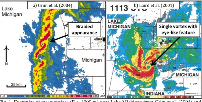
Previous lake-effect research field campaigns have primarily focused on the Western Great Lakes, such as Lakes Michigan and Superior [e.g., the Lake-Induced Convection Experiment (Lake-ICE); Kristovich et al. (2000)]. Some of these studies, including Forbes and Merritt (1984) and Laird et al. (2001), document instances of mesovortices [diameters (D) > 4000 m; Fujita 1981] forming over the lakes in regimes of weak background synoptic flow (e.g., Niziol et al. 1995, Type-V bands). The mesovortices typically either exhibit a braided structure (Fig. 1a; Grim et al. 2004) or occur as a single vortex with an eye-like feature (Fig. 1b; Laird et al. 2001) on radar and visible satellite imagery. The formation of mesovortices is largely governed by latent heat release owing to depositional processes within the band, inducing rising heights and divergence above the level of maximum heating and falling pressures below this level (e.g., Laird et al. 2001). The lower pressure near the lake surface, in turn, induces low-level cyclonic rotation and the formation of a mesovortex.
The first large-scale field campaign over the Eastern Great Lakes was the Lake Ontario Winter Storms (LOWS; Reinking et al. 1993) Project. This field campaign was centered across the Lake Ontario region and was conducted between 5 January and 1 March 1990. The main goal of the project was to improve short-term (0-12 h) forecasts of lake-effect snow and synoptically-forced freezing rain events. Due to the dearth of major cold air intrusions across the Great Lakes within the timeframe of the field campaign, however, only one LLAP band case was sampled and analyzed, occurring on 12 January 1990.
Reinking et al. (1993) simulated this band using the State University of New York (SUNY) at Oswego Mesoscale Model (Ballentine 1980) with 10-km horizontal grid spacing. The
3
simulation revealed a warm-core structure within the band with low-level convergence extending to an altitude of 0.5 km above ground level (AGL) and divergence near the top (~675 hPa) of the band (i.e., an in-up-and-out transverse vertical circulation). While the model captured the general mesoscale structure of the band, the simulation grossly underestimated the depth of the planetary boundary layer (PBL). The PBL height extended to an altitude between 1.2 and 2.5 km AGL in the simulation, compared to 4 km AGL in mobile soundings. An important discovery was that the depth of the PBL appeared to be a more important indicator of band intensity than the lake surface-to-850 hPa temperature difference. This agrees with the results from an observational study by Byrd et al. (1991).
The modeling results from the LOWS campaign are comparable to a Weather Research and Forecasting (WRF-NMM; 8-km horizontal grid spacing with 31 vertical levels) model simulation of a LLAP band that occurred between 3-12 February 2007, which produced over 350 cm of snowfall at Redfield, NY (Steiger and Ballentine 2008). Figure 2a displays the WRF model-simulated composite reflectivity and 10-m winds at 0800 UTC 5 February 2007. The north-south vertical cross-section (Fig. 2b, along the solid black line in Fig. 2a) depicts low-level convergence near the center of the band, ascent within the core of the band, and divergence atop the band. This transverse vertical circulation is strikingly similar to that obtained in the analyses from the LOWS Project. These band-induced, low-level convergence zones are common in LLAP bands and may be augmented by land-breezes from opposing shores as surrounding land locations are usually significantly cooler than the lake surface (especially before sunrise; Passarelli and Braham 1981). The narrow corridor of enhanced low-level convergence aids in the development of a ribbon of convective updrafts within the band (Fig. 2b). Additionally, potential temperature surpluses of 2-3 K were noted within the center of the simulated bands on both 12
4
January 1990 and 5 February 2007. This warm-core structure compares remarkably well with the Byrd et al. (1991) study, which found maximum positive temperature perturbations of 2.5 K at an altitude of 2 km AGL within a LLAP band.
A more recent field campaign, the Long Lake-Axis-Parallel (LLAP; Steiger et al. 2013) Project, occurred during the winter of 2010-2011 across Lake Ontario and surrounding downwind locations. This project featured many more observations of LLAP bands than did the LOWS Project (7 events during LLAP vs. 1 event during LOWS). The main goal of the LLAP Project was to obtain fine-scale, dual-polarization, mobile Doppler radar observations of LLAP bands. Observations of mesovortices (Figs. 3a, b; D > 4000 m), misovortices (Fig. 3c, d; D ~ 40-4000 m), horizontal vortices, horizontal shear zones (Fig. 3d), bounded weak echo regions, outflow boundaries, and anvils were all documented (Steiger et al. 2013). The mesovortices, which at times exhibited a reflectivity structure similar to supercell hook echoes, sometimes altered the morphology and orientation of the bands. This has the potential for major implications for operational forecasters attempting to predict snowfall intensity, amount, and location. Additionally, Steiger et al. (2013) observed that the LLAP bands typically displayed an asymmetric structure with a sharper horizontal reflectivity gradient on either the north or south side of the typically west-to-east oriented bands. This gradient is hypothesized to be near the location of the largest upward vertical velocities, where hydrometeor lofting is manifested by lower values of radar reflectivity near the surface. On the same side of the band as the reflectivity gradient, and along the corresponding horizontal shear/convergence zone, there were several smaller-scale vortices observed (D < 4000 m), which were roughly evenly spaced. The primary formation mechanism for these misovortices was hypothesized to be the release of horizontal shearing instability (HSI; Markowski and Richardson 2010, p. 58-64) along the cyclonic
5
horizontal shear zone. This hypothesis was not testable, however, since only a single Doppler radar was available, precluding a dual-Doppler wind synthesis. No LLAP cases that the author is aware of exhibited an anticyclonic shear zone. A more detailed investigation of this hypothesis, along with prior research on HSI-induced vortices, is found in Chapters 4 and 5.
The largest project of its kind, the Ontario Winter Lake-effect Systems (OWLeS; Kristovich et al. 2016) Project, occurred during the winter of 2013-2014. Stemming from the successes of the exploratory LLAP Project, the three main objectives of the OWLeS Project were to examine: 1) The kinematics and dynamics of LLAP bands, 2) Upwind and downwind lake influences (i.e., heat and moisture fluxes and advection) on lake-effect convection, and 3) Orographic influences on lake-effect convection. The original OWLeS proposal planned for eight intensive observation periods (IOPs), whereas twenty-four IOPs took place owing to a persistent pattern characterized by high-amplitude ridging across the Western U.S. and deep troughing across the Eastern U.S. (see Chapter 3). The full list of instrumentation utilized during this field campaign is located in Chapter 2, section 1.
This research herein is focused on the first objective of the OWLeS field campaign, and more specifically attempts to understand the underlying kinematics and dynamics that aid in the development, maintenance, and ultimate demise of the misovortices documented within the 7 January 2014 LLAP band. Steiger et al. (2013), along with OWLeS Project field observations, have demonstrated that the larger-scale mesovortices have the ability to alter the morphology of LLAP bands, while the smaller-scale misovortices were typically associated with localized maxima in surface wind speeds and snowfall rates (also noted by Grim et al. 2004). Hence, this research may be particularly useful to operational forecasters concerned with forecasting snowfall amounts, locations, and intensities associated with these LLAP bands.
6
Chapter 2 outlines the data and methodology used during this research. Chapter 3 provides an analysis of the synoptic and mesoscale conditions present on 7 January 2014. Chapter 4 reveals the DD observations of the misovortices. Chapter 5 includes an analysis of a high-resolution WRF model simulation of this band, and summary and conclusions are found in Chapter 6.
7 1.1 Figures
Fig. 1. Examples of mesovortices (D > 4000 m) over Lake Michigan from Grim et al. (2004) and Laird et al. (2001). Radar reflectivity (dBZ; shaded) at 0.5˚ from Grand Rapids, MI (KGRR), valid at a) 1517 UTC 14 January 2003 and b) 1113 UTC 5 December 1997.
8
Fig. 2. Weather Research and Forecasting (WRF) simulation valid at 0800 UTC 5 February 2007 showing: a) composite reflectivity (dBZ; contoured in black every 5 dBZ), 10-m winds (kts; barbs; half barb = 5 kts, full barb = 10 kts), Interstate highways (red lines), state and U.S. highways (green lines), and county borders (orange lines); and b) north-south vertical cross-section [111 km along the solid black line in (a)] depicting composite reflectivity (dBZ; contoured in green every 5 dBZ), potential temperature (K; contoured in blue every 1 K), equivalent potential temperature (K; contoured in red dashed lines every 1 K), wind vectors (black arrows; length proportional to wind speed), and two representative streamlines (heavy dashed black arrows). [The dashed west-east cross-section line in (a) is not shown].
a)
9
Fig. 3. DOW7 observations of a) reflectivity (dBZ) and b) radial velocity (m s-1) at 03:17:58 UTC 5 January 2011, and c) reflectivity (dBZ) and d) radial velocity (m s-1) at 07:00:05 UTC 16 December 2010. The yellow star denotes the location of DOW7. Tick marks are spaced every 5 km (Figure adapted from Steiger et al. 2013).
10 CHAPTER 2
DATA AND METHODOLOGY 2.1 Observational Data
The platforms that were utilized during the OWLeS Project included: Three X-band Doppler-on-Wheels (DOW; Wurman et al. 1997) radars (two dual-polarization), five (four mobile) rawinsonde systems (SUNY Oswego, University of Utah, University of Illinois at Urbana-Champaign, Millersville University, and Hobart and William Smith Colleges), the University of Wyoming King Air (UWKA) aircraft, and the University of Alabama in Huntsville’s Mobile Integrated Profiling System (MIPS). Radar data from 7 January 2014 were collected using two mobile X-band DOW radars (DOW6 and DOW8-Rapid Scan), the specifications for which are listed in Tables 1 and 2 below. The radars were deployed between 0200-2230 UTC 7 January 2014. DOW6 was stationed at Rainbow Shores, NY, while DOW8 was stationed at Southwick Beach, NY, resulting in a DD lobe over Eastern Lake Ontario (Fig. 4; radar baseline of 16.4 km). The locations of the remaining mobile assets are also shown in Fig. 4.
2.2 Dual-Doppler Analysis
Raw DOW data were first subjectively edited using SOLO-III software. All radar data to the east of Lake Ontario were removed owing to beam blockage resulting from tree cover along the shoreline. Using a cross-correlation coefficient (
ρ
HV; Fabry 2015, p. 99-101) threshold of 0.94(which, according to Fabry 2015, is representative of non-meteorological targets in a typical dry snow environment), ground clutter within the DOW6 dataset was removed, including sea spray/clutter, the shoreline imprint of Lake Ontario, buildings, trees, and other
non-11
meteorological targets. Additionally, gates with radial velocity magnitudes greater than +5 m s-1 to the west of the radar were removed since the boundary-layer flow was westerly across the entire domain for the duration of the event, even north of the cyclonic vortices. A similar editing process was applied to data from DOW8. Since DOW8 is not a dual-polarization radar, however, ground clutter was filtered using high reflectivity values (generally above 25 dBZ used as threshold), co-located with zero radial velocity magnitudes that were clearly not associated with precipitation. Other noise was removed by thresholding on normalized coherent power (NCP; Dixon and Hubbert 2012). An NCP value of 0.30 (for areas outside of the string of vortices) was used to identify regions of low signal, and pixels with a value below this threshold were removed from the dataset. All other non-meteorological targets or noise that remained were manually removed at the conclusion of the editing process.
Using a two-pass Barnes objective analysis (Barnes 1964), the edited data were mapped to a 40 x 40 x 2.5 km Cartesian grid with a horizontal and vertical grid spacing of 250 m, consistent with the recommendations from Pauley and Wu (1990), where Δx, Δy, Δz = 5𝛿12 and 𝛿 = (0.93˚)(π/180˚)(X), where X is the greatest distance from one of the radars to a feature of interest in km. The Barnes smoothing parameter is given by Κ = (1.33𝛿)2, also consistent with recommendations by Pauley and Wu (1990) and Marquis et al. (2007). The horizontal smoothing parameter (ΚH) is 0.747 km
2
while the vertical smoothing parameter (ΚZ) is 0.400 km 2
. Scans between 1-2˚ from DOW8 were missing because one of the X beams was nonfunctional, necessitating the difference in the horizontal and vertical smoothing parameters mentioned above. The origin of the Cartesian grid was the location of DOW6. Three-dimensional wind syntheses were obtained from the objectively-analyzed radar data by integrating the anelastic mass continuity equation upward from the bottom of the domain using OPAWS software (with
12
the assumption that w = 0 at the bottom of the domain). From these DD wind syntheses, fields such as vertical velocity and vertical vorticity were calculated and analyzed (see Chapter 4).
2.3 Weather Research and Forecasting (WRF) Model Specifications
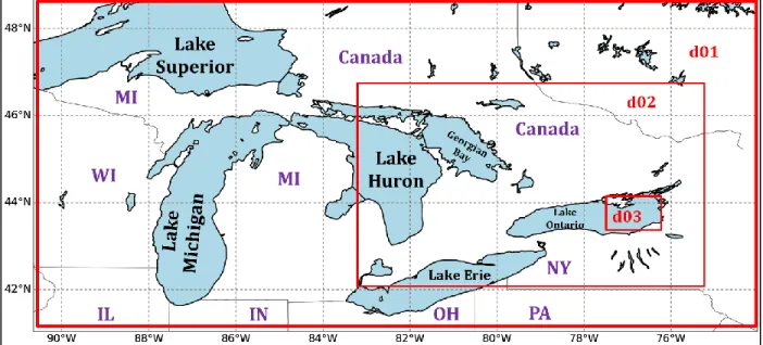
A Weather Research and Forecasting (WRF-ARW; version 3.7.1) model simulation was conducted for this case. The innermost grid had a horizontal resolution of 333 m (258 x 147 km) and was nested within 1 km (636 x 438 km) and 3 km (1335 x 882 km) grids. The outermost domain (3 km horizontal resolution) was initialized from the 0000 UTC 7 January 2014 Rapid-Refresh (RAP) model. The model domains are depicted in Fig. 5. The 3-km domain was used to equilibrate the synoptic-scale features across the Great Lakes Region, while the 1-km domain was centered on Georgian Bay and Lake Ontario to capture a connection between the LLAP band originating over Georgian Bay and that over Lake Ontario (see Chapter 3). The finest-scale (333 m) domain only encompassed Eastern Lake Ontario to reproduce the misovortices which were observed in the mobile radar data. The 333-m grid spacing is comparable to the 250-m horizontal resolution of the DD grid, allowing for a nearly one-to-one comparison of vortex characteristics including vortex strength, spacing, and depth.
The model simulation utilized 60 vertical levels with a vertical, terrain-following eta-coordinate. The top of the model domain was at 50 hPa, approximately 20 km AGL. No damping layer was implemented near the model top owing to the relatively shallow depth of the lake-effect convection (< 5 km AGL) and short duration of the model integration (12 h). A vertically-stretched grid was utilized, with the lowest model level located at 75 m AGL. The vertical grid resolution near the surface is 35 m and decreases to approximately 750 m near the model top. The model was run on the Arakawa C-grid and Runge-Kutta 2nd and 3rd order time integration
13
schemes were utilized. The Morrison two-moment microphysical scheme (Morrison et al. 2009) was utilized along with the Rapid Radiative Transfer Model GCM (RRTMG) longwave and shortwave radiation schemes (Iacono et al. 2008), the Rapid Update Cycle (RUC) land surface model (LSM; Smirnova et al. 2016), the revised Pennsylvania State University (PSU)/National Center for Atmospheric Research (NCAR) Mesoscale Model (MM5) Monin-Obukov surface layer scheme (Jiménez et al. 2012), and the Yonsei University (YSU; Hong et al. 2006) boundary-layer parametrization. For the 3-km and 1-km domains, the new Kain-Fritsch cumulus parametrization scheme (Kain 2004) was implemented. A summary of the model configuration is found in Table 3.
14 2.4 Figures and Tables
Doppler-on-Wheels (DOW6) radar specifications. Half-power beamwidth 0.5˚ Frequency 9.55 GHz Gate length 60 m Transmitter pulse 400 ns Nyquist velocity 78.47 m s-1 Maximum range Elevation angles 60 km 0.5 - 14.5˚ Table 1. DOW6 radar specifications during the 7 January 2014 event.
Doppler-on-Wheels (DOW8-Rapid Scan) radar specifications. Half-power beamwidth 0.5˚ Frequency 9.55 GHz Gate length 75 m Transmitter pulse 1000 ns Nyquist velocity 31.97 m s-1 Maximum range Elevation angles 60 km 0.5 - 14.9˚ (missing 1-2˚) Table 2. DOW8 radar specifications during the 7 January 2014 event.
15
Fig. 4. OWLeS asset map from 7 January 2014. The dual-Doppler lobe from DOW6 and DOW8 is drawn in red; the radar baseline is 16.4 km. The locations of DOW6 and DOW8 are marked with yellow circles (DOW8 to the north, DOW6 to the south), the Montague, NY (KTYX), WSR-88D radar location is labeled and marked with a red circle, mobile snow-sampling teams are labeled and marked with white asterisks, Microwave Rain Radars (MRR) are labeled and marked with blue rain drops, and the mobile sounding locations are labeled and marked with a variety of colors/symbols (HWS, SUNYO, UTAH, and MU).
Dual-Doppler
Lobe
16
Weather Research and Forecasting (WRF) model specifications.
Horizontal grid spacing 3 km, 1 km, 333 m
Vertical levels 60
Vertical coordinate ɳ (terrain-following)
Ptop 50 hPa
Microphysical parameterization Morrison two-moment
Boundary-layer scheme YSU
LW and SW radiation scheme Surface-layer scheme
Land surface scheme
RRTMG
MM5 Monin-Obukov RUC LSM Table 3. WRF model specifications. Abbreviations are explained in the text.
Fig. 5. Domains of the Weather Research and Forecasting (WRF) model simulation. The outermost domain (d01; 1335 x 882 km) has a horizontal grid spacing of 3 km, the middle domain (d02; 636 x 438 km) has a horizontal grid spacing of 1 km, while the innermost domain (d03; 258 x 147) has a horizontal grid spacing of 333 m.
17
CHAPTER 3
7 JANUARY 2014: SYNOPTIC AND MESOSCALE OVERVIEW
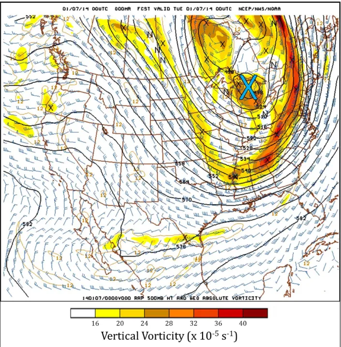
Throughout the winter of 2013-2014, frequent intrusions of Arctic air masses occurred over most of the Eastern United States. One such event took place between 6-9 January 2014, with some locations east of Lake Ontario receiving over 125 cm (> 50”) of fresh snowfall (Fig. 6). The 0000 UTC 7 January 2014 Rapid Refresh (RAP) model 500-hPa analysis reveals a highly-amplified pattern with a deep trough over Eastern North America and a ridge across Western North America (Fig. 7). A shortwave trough was located to the west of Lake Ontario, over Northern Lower Michigan (denoted by the blue “X” in Fig. 7), which traversed Lake Ontario between 0400-0800 UTC. Quasi-geostrophic ascent due to differential positive vorticity advection ahead of this trough overspread the region, forcing the capping inversion atop the Arctic air mass over Lake Ontario to rise. Soundings launched at 0513 UTC and 0816 UTC from Henderson Harbor, NY, depicted the midlevel cooling and vertical extension of the boundary layer in association with the synoptic-scale ascent overspreading the region (Fig. 8). The 0816 UTC sounding reveals a moist and conditionally-unstable boundary-layer extending vertically to nearly 540 hPa (Fig. 8; blue line). With 850-hPa temperatures around -25˚C, lake-surface water temperatures around 3˚C, and a nearly unidirectional wind profile with height, thermodynamic and kinematic conditions were more than adequate for an intense LLAP band to develop over Lake Ontario (Fig. 9).
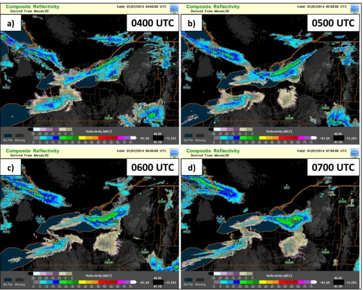
Further inspection of the mesoscale regime revealed a connection between the Lake Ontario band and another LLAP band upstream over Georgian Bay that lasted from 0400-0800 UTC (Fig. 9). This connection ceased after 0800 UTC as boundary-layer winds over Georgian Bay backed from northwesterly to westerly following the passage of the aforementioned 500-hPa
18
shortwave trough and the approach of a 700-hPa ridge from the west (see Chapter 5, section 1). The advection of heat and moisture from upstream lakes enhancing downwind lake-effect storms has been well documented in the literature (e.g., Byrd et al. 1991; Sousounis and Mann 2000; Rodriguez et al. 2007). These multilake connections are commonly observed across the Great Lakes during instances of northwest boundary-layer flow in which a single snow band may be traced across as many as three lakes.
The Lake Ontario LLAP band persisted for over 20 h during the 6-7 January 2014 period, even after the upstream connection was lost. The analysis, located in Chapters 4 and 5, is focused between 0400-0800 UTC, since this was when the string of misovortices was present. Isolated vortices were observed after 0800 UTC, but strings of vortices were not observed.
19 3.1 Figures
Fig. 6. Total accumulated snowfall (inches) between 6-9 January 2014 (Courtesy: National Weather Service Forecast Office in Buffalo, NY).
20
Fig. 7. Rapid Refresh (RAP) model 500-hPa analysis valid at 0000 UTC 7 January 2014. Geopotential height is in solid black contours (every 6 Dm), winds (kts; barbs; half barb = 5 kts, full barb = 10 kts, flag = 50 kts) are in blue, and geostrophic absolute vorticity (shaded every 4 x 10⁻⁵ s-1 starting at 16 x 10-5 s-1). The blue “X” denotes the location of the shortwave trough that traversed Lake Ontario during this event (Figure courtesy: OWLeS Field Catalog; Available online at http://catalog.eol.ucar.edu/owles).
21
Fig. 8. Soundings launched at 0513 UTC (red) and 0816 UTC (blue) 7 January 2014 from Henderson Harbor, NY. Horizontal winds (m s-1; barbs; half barb = 2.5 m s-1, full barb = 5 m s-1, flag = 25 m s-1) for both soundings are plotted along the right side of the image.
22
Fig. 9. Multi-Radar Multi-Sensor (MRMS; available online at http://mrms.ou.edu/) System composite reflectivity (dBZ) and terrain (grayscale background) valid at: a) 0400 UTC, b) 0500 UTC, c) 0600 UTC, and d) 0700 UTC 7 January 2014.
a) b)
23 CHAPTER 4
RESULTS: DUAL-DOPPLER ANALYSES 4.1 Vortex Characteristics
Between 0400-0800 UTC 7 January 2014, a string of misovortices was observed within the LLAP band. At the beginning of this timeframe, the band was cyclonically curved, likely owing to cyclonic boundary-layer flow attributable to the passing midlevel shortwave trough. Figure 10 depicts the string of misovortices at 0524 UTC, with diameters (defined here as the distance between local maximum/minimum values of velocity that are coincident with a maximum in vertical vorticity, as in Steiger et al. 2013) ranging from 1 - 3 km and an average horizontal spacing around 6.5 km. The misovortices were located along the northern edge of the band, near a sharp north-south horizontal gradient in reflectivity (Fig. 10a). This region was also characterized by a cyclonic horizontal shear zone, evidenced by the faster inbound velocities (darker green and purple colors; on the order of 20 m s-1) to the south of the misovortices and the slower inbound velocities (lighter green colors; on the order of 10 m s-1) to the north of the misovortices (Fig. 10b). Furthermore, locally stronger zonal winds were commonly observed to the south of the cyclonic vortices, with weaker zonal winds to the north of the vortices.
Figure 11, valid at 0744 UTC, reveals fewer misovortices over Lake Ontario than a few hours earlier. The shear zone had moved closer to the center of the band, with the edges of the band appearing more diffuse in the reflectivity field. The band had also lost its earlier cyclonic curvature and had become oriented WNW to ESE as the midlevel shortwave trough ejected to the northeast. This transition occurred 1-2 h after the initial backing of the boundary-layer winds upstream over Georgian Bay and the subsequent cessation of the connection with the Georgian Bay band. The string of misovortices in this particular case may have depended on Georgian
24
Bay; once the connection ceased, the string of misovortices vanished and instances of only isolated vortices prevailed throughout the remainder of the event (hence why DD analyses were only performed between 0400-0800 UTC). Observations from the King City, Ontario (CWKR), radar site depict a cyclonic horizontal shear zone downwind of Georgian Bay, oriented southeastward toward Lake Ontario (Fig. 12). This shear zone is thought to be the impetus for the initiation of the misovortices over Lake Ontario. Analyses from a high-resolution WRF simulation of the morphology of this vortex sheet are located in Chapter 5.
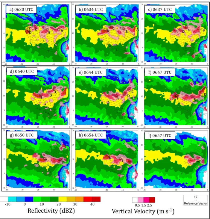
Figure 13 displays a 27-minute (0630-0657 UTC), DD-derived time evolution of the string of misovortices (each labeled with a letter, A through G). The vortices throughout this time period were located within the northern half of the band, along a sharp north-south horizontal gradient in reflectivity, and could be tracked for greater than 30 minutes. Vertical vorticity values within the vortices throughout this time period ranged from 1.0 - 3.0 x 10⁻² s-1 and are within the range of those documented by other studies that analyzed misovortices (e.g., Wilson et al. 1992; Lee and Wilhelmson 1997; Kawashima and Fujiyoshi 2005; Arnott et al. 2006; Buban et al. 2007; Marquis et al. 2007; Campbell et al. 2014). For example, DD analyses of misovortices along low-level convergence zones observed over the Southern Great Plains during the International H2O Project (IHOP_2002; Weckwerth et al. 2004), exhibited vertical
vorticity values between 0.6 - 2.0 x 10⁻² s-1 (e.g., Arnott et al. 2006; Marquis et al. 2007). An earlier study by Mueller and Carbone (1987) observed misovortices along a thunderstorm outflow boundary and their results exhibit values of vertical vorticity between 3.0 - 5.3 x 10⁻² s-1. Vortices A-E were tracked between 0630-0657 UTC and exhibit an average propagation speed of 19 m s-1 toward the ESE. The average horizontal spacing between the vortices during this time period was on the order of 5.6 km, which is about 1 km less than at 0524 UTC (Fig.
25
10). The vortices exhibit pulse-like fluctuations in intensity, similar to what was noted in idealized simulations conducted by Buban and Ziegler (2015). The DD analyses of the vortices in this study would not benefit from linear stability analysis techniques that relate the initial vortex sheet width to the horizontal spacing of the vortices (e.g., Miles and Howard 1964; Lee and Wilhelmson 1997) because the present analyses occur during the mature phases of the vortices and not during their incipient stages of development. Furthermore, there has not been a universal method for defining the initial shear zone width; hence, further vortex spacing analyses have been left to future research.
Vortices C-E at 0640 UTC were initially oriented WSW to ENE along the northern edge of the band (Fig. 13d), however, 10 minutes later, vortices E and F became oriented WNW to ESE, closer to the center of the band (Fig. 13g). This shift in the orientation of the string of vortices is coincident with the beginning stages of the cessation of the connection with the upstream LLAP band, which began to lift northward in tandem with the approach of the midlevel shortwave ridge. After this time, the vortices weakened markedly, and by 0744 UTC, the string of vortices was no longer present.
The updrafts along the confluence axis exhibit maximum values between 1 - 3 m s-1 (Fig. 13). In some instances, the center of an updraft overlapped with a misovortex (e.g., Fig. 13b, Vortex C), however, sometimes the two were separated (e.g., Fig. 13d, Vortex D). This line of updrafts was co-located with enhanced near-surface convergence and band-top divergence associated with the transverse secondary circulation of the band, as depicted in plots of the meridional wind at 500 and 2000 m AGL (Figs. 14 and 15). The depth of this circulation reached at least 2 km AGL (near the top of the DD domain). The magnitude of this circulation weakened between 0630 to 0744 UTC, at the same time the vortices were observed to weaken.
26
Characteristic values of 500-m AGL horizontal convergence along this boundary were between 3 - 5 x 10⁻³ s-1 (Fig. 16). Regions of locally-enhanced low-level convergence and upward motion were generally observed NE and SW of each vortex, with the strongest vortices exhibiting near-zero convergence (or sometimes weak divergence) within their centers, while weaker vortices exhibited a more uniform convergence signature within each vortex (Figs. 13 and 16). This observation is similar to the findings of Marquis et al. (2007), who analyzed misovortices along Southern Great Plains drylines (see also Arnott et al. 2006). Their conceptual model of a convergence boundary superposed with misovortices matches the findings in the present study (Fig. 17). Marquis et al. (2007) postulate that the convergence along the vortex sheet may be enhanced by the vortices through an additive effect of the boundary-induced convergence and the vortex-induced convergence. This convergence configuration relative to the vortex centers has been noted in other studies as well, including Kingsmill (1995) and Lee and Wilhelmson (1997).
A south-to-north vertical cross-section through one of the vortices at 0630 UTC is depicted in Fig. 18 (taken along green line in Fig. 16). This vortex is strongest between 0.5 - 1.0 km AGL and weakens with height above 1 km. This vortex also tilts toward the south with height because winds above 1.5 km AGL become more northerly (Fig. 18). The updraft is north of the vortex center; however, updraft magnitudes between 1 - 3 m s-1 still overlap with vertical vorticity values greater than 0.7 x 10⁻² s-1. This is not the case for all vortices, however, as some exhibit a greater overlap between the updraft and positive vertical vorticity (Fig. 13). The juxtaposition between low-level upward motion and vertical vorticity further enhances vertical vorticity via stretching, which is described by the vertical vorticity tendency equation below:
𝜕𝜁
𝜕𝑡 = 𝑣⃗ ∙ ∇ζ + 𝜔⃗⃗⃗𝐻∙ ∇𝑤 + 𝜁 𝜕𝑤
27
where 𝜁 is vertical vorticity (s-1), 𝑡 is time (s), 𝑣⃗ is the velocity vector (m s-1), 𝜔⃗⃗⃗𝐻 is the horizontal vorticity vector (s-1), 𝑤 is vertical velocity (m s-1), and 𝑧 is height (m). Neglecting advection and tilting and solving this equation for 𝜁 yields:
𝜁 = 𝜁𝑜 exp (𝜕𝑤𝜕𝑧𝑡) (2)
where 𝜁𝑜 is the initial vertical vorticity (s-1). In the presence of preexisting vertical vorticity, stretching amplifies vertical vorticity exponentially in time, allowing for intensification of the misovortices. Further discussion on potential formation mechanisms of these misovortices is located in the next section.
By 0744 UTC (Fig. 14f), the lack of a string of vortices is noted, which is in stark contrast to what was observed around 0630 UTC (Fig. 14a), and even earlier (not shown). This transition to a regime characterized by a general lack of vortices followed the passage of the 500-hPa shortwave trough and approach of the 700-500-hPa ridge, and the termination of the connection with Georgian Bay (as discussed in Chapter 3). The vertical vorticity and horizontal convergence values decreased along the shear zone by 0744 UTC and were only on the order of 0.8 x 10⁻² s-1 (Fig. 14f) and 1 - 3 x 10⁻³ s-1 (Fig. 16f), respectively. The maximum vertical velocity values had also decreased to around 1 m s-1, from earlier values between 1.5 - 3.0 m s-1. This decrease in the band-induced, mesoscale updraft strength likely restricted subsequent amplification of vertical vorticity within the vortices via vortex stretching. After 0744 UTC, only isolated instances of misovortices were observed throughout the remainder of the event (not shown).
4.2 Horizontal Shearing Instability (HSI)
The development of strings of misovortices has been attributed to the release of horizontal shearing instability (HSI) based on both observational (e.g., Mueller and Carbone
28
1987; Marquis et al. 2007) and modeling studies (e.g., Lee and Wilhelmson 1997; Buban and Ziegler 2015). Boundaries featuring large horizontal wind shear, such as drylines, cold fronts, and outflow boundaries, can be favored regions for misovortexgenesis (Markowski and Richardson 2010, p. 58-64). Greater magnitudes of across-boundary shear can result in stronger misovortices (e.g., Lee and Wilhelmson 1997; Friedrich et al. 2005). The misovortices in this case developed along a nearly west-to-east oriented cyclonic horizontal shear/convergence zone within the northern half of the band.
In an attempt to support the hypothesis that HSI was the main driver for the development of the misovortices observed in this case, two HSI conditions were analyzed. The first condition, Rayleigh’s Stability Criterion (Rayleigh 1880), states that 𝛽 −𝜕𝜕𝑦2𝑢̅2 must change sign somewhere within the flow (see Markowski and Richardson 2010, p. 63-64, for a full derivation), where 𝛽 = 𝑑𝑓
𝑑𝑦, 𝑓 is the Coriolis parameter (s
-1
), 𝑦 is the meridional direction (m), and 𝑢̅ is the zonally-averaged zonal wind (m s-1). Assuming 𝑓 = 10-4 s-1 and 𝑦 = 107 m, 𝛽 is of order 10-11 m-1 s-1. A simple scale analysis of the quantity 𝜕
2𝑢̅
𝜕𝑦2, using an approximate Δ𝑢̅ = 10 m s -1
and Δ𝑦 = 10 km, returns a value on the order of 10-7 m s-1 (approximately 4 orders of magnitude larger than 𝛽). Hence, we can ignore 𝛽 on the mesoscale, leaving the sign change of the term 𝜕
2𝑢̅
𝜕𝑦2 as the
instability criterion. In other words, there must be an inflection point within the 𝑢̅ profile for HSI to be present. A more stringent condition, derived by Fjørtoft (1950), states that 𝜕𝜕𝑦2𝑢̅2(𝑢̅ − 𝑢̅𝐼) < 0 for instability, where 𝑢̅𝐼is the mean base state zonal wind at the inflection point (found from Rayleigh’s Stability Criterion above). These are both necessary, but insufficient conditions for instability, however.
29
An analysis of the zonal wind at 500 m AGL depicts the cyclonic horizontal shear zone along which the misovortices are found (Fig. 19). Figure 20a, at 0630 UTC, depicts the zonally-averaged 𝑢̅ profile, as a function of y, with an inflection point (green dot labeled I.P.) at y = 13 km. This inflection point corresponds to the location of the shear zone and the vortices in Fig. 20b. There is also a sign change in 𝜕
2𝑢̅
𝜕𝑦2 at y = 13 km (Fig. 21a). Hence, Fig. 21a illustrates that
Rayleigh’s Stability Criterion is met along the shear zone. There are other locations that satisfy Rayleigh’s Stability Criterion, such as at y = 4 km (Fig. 21a), however, this is not within the shear zone and may result from noise near the edges of the DD domain. A triangular-weighted smoother (Wittenberg 2009) was applied to these data in order to reduce some of this smaller-scale noise that results from calculating higher-order derivatives.
Inspection of Rayleigh’s Stability Criterion between 0644-0744 UTC (Figs. 21b-f) reveals that this condition for instability is met at each of these successive times with a clear sign change of the quantity 𝜕
2𝑢̅
𝜕𝑦2 near the horizontal shear zone and vortices (given by the red dashed
lines in Fig. 21). The fact that at each analysis time this instability criterion was satisfied along the shear zone strongly supports the hypothesis that HSI was the primary mechanism for misovortexgenesis in this case.
Fjørtoft’s Stability Criterion [ 𝜕𝜕𝑦2𝑢̅2 (𝑢̅ − 𝑢̅𝐼) < 0 ] is plotted in Fig. 22 for the same time period (0630-0744 UTC). This quantity will be exactly zero at the location of 𝑢̅𝐼, hence this criterion is met if negative values bound the 𝑢̅𝐼 location. An example of where this more stringent criterion is met is between y = 9 km and y = 16 km at 0630 UTC (Fig. 22a), which is the same region where the shear zone and vortices are present, and also where Rayleigh’s Instability Criterion is satisfied (compare Figs. 21a and 22a). Additional analyses of Fjørtoft’s
30
Stability Criterion between 0644-0744 UTC are depicted in Figs. 22b-f. Each plot displays that this more stringent instability criterion is satisfied at the location of the shear zone and vortices, and also where Rayleigh’s Stability Criterion is met, further supporting the hypothesis that HSI is the driving mechanism for the formation of the misovortices during this case. Without DD analyses of misovortex development, however, it is impossible to determine definitively the formation mechanism for these misovortices (e.g., see Marquis et al 2007).
Additional theories of misovortexgenesis include the production of vertical vorticity via tilting of horizontal vorticity by updrafts. Studies such as Arnott et al. (2006) postulated that vertical vorticity within misovortices may have originated from horizontal vorticity that was initially tilted and then advected vertically. Lee and Wilhelmson (1997) demonstrate that surface roughness also generates low-level horizontal vorticity that may subsequently be tilted and aid in the development of their simulated vortices. A study of misocyclones in Northeastern Colorado (Wilczak et al. 1992) demonstrates through a vorticity budget that tilting of horizontal vorticity played a vital role in the formation of their observed misocyclones. These studies, however, have primarily examined vortices along baroclinic boundaries (e.g., cold fronts), in which vertical wind shear is arguably larger than the fairly uniform temperature field over the lake surface (e.g., Arnott et al. 2006).
A vorticity budget calculated from the DD analyses is depicted in Figs. 23 and 24, respectively. Values of tilting (between -0.30 and 0.30 x 10⁻⁴ s-2) are considerably less than values of stretching (between -1.50 and 1.50 x 10⁻⁴ s-2). The tilting term tends to be maximized along the edges of the vortices and above 1.5 km AGL (not shown), owing to the relatively large horizontal gradient in vertical velocity surrounding each updraft (Fig. 23). The stretching term, however, is maximized within the cores of the vortices where a maximum in vertical vorticity
31
exists in the presence of upward vertical velocity (Fig. 24). A similar arrangement of tilting vs. stretching relative to misovortices was also noted in the simulations by Lee and Wilhelmson (1997). In some instances, the vortices are characterized by negative values of tilting within their cores (e.g., Fig. 23c). This observation is similar to one noted by Buban and Ziegler (2015), who deduced that negative tilting of preexisting vertical vorticity into the horizontal occurred within their simulated vortices. Additionally, Buban and Ziegler (2015) have also revealed that stretching dominates tilting in their simulations. Finally, tilting alone cannot describe the local maxima in vertical vorticity near the surface as vertical advection within updrafts will result in the largest values of vorticity being displaced upward (e.g., Davies-Jones 1982a,b).
The lack of anticyclonic-cyclonic vortex couplets straddling the linear updraft region further implies that tilting is likely muted relative to the release of HSI and subsequent vortex stretching (e.g., Wheatley and Trapp 2008; see also Fig. 25). Furthermore, horizontal gradients in vertical velocity are typically smaller in magnitude in lake-effect storms (e.g., this case ~1 m s-1 over 1 km) as compared to previously-studied misovortex environments over the Great Plains and Florida (e.g., ~3 m s-1 over 1 km; Arnott et al. 2006), and certainly relative to much more robust supercellular convection (e.g., ~10 m s-1 over 1 km; Brooks and Wilhelmson 1993). Thus, our analyses of the 7 January 2014 lake-effect band support the hypothesis proposed by Steiger et al. (2013) that the governing mechanism for misovortexgenesis in LLAP bands, at least in this particular case, is the release of HSI and subsequent strengthening via low-level vortex stretching. In this case, the presence of vortices also appears to be strongly linked to the connection with the Georgian Bay band. More analyses regarding the importance of this connection are discussed in Chapter 5.
32 4.3 Figures
Fig. 10. 0.4˚ DOW6 radar, a) reflectivity (dBZ) and b) radial velocity (m s-1) at 05:23:55 UTC 7 January 2014. Range rings are plotted every 5 km and azimuth angles are plotted every 30˚. Each misovortex is denoted by a red arrow.
Fig. 11. 0.5˚ DOW6 radar, a) reflectivity (dBZ) and b) radial velocity (m s-1) at 07:43:55 UTC 7 January 2014. Range rings are plotted every 5 km and azimuth angles are plotted every 30˚.
a) DOW6 Ref (dBZ) b) DOW6 Vel (m s-1)
33
Fig. 12. 0.2˚ King City, Ontario (CWKR), radar, a) reflectivity (dBZ) and b) radial velocity (m s-1) at 05:23:35 UTC 7 January 2014. Range rings are plotted every 10 km and azimuth angles are plotted every 30˚. The black oval denotes the location of the cyclonic horizontal shear zone discussed in the text.
34
Fig. 13. Dual-Doppler wind synthesis at 500 m AGL with horizontal wind vectors (black arrows; m s-1), vertical vorticity (only positive values shown; contoured every 0.4 x 10⁻² s-1 starting at 0.6 x 10⁻² s-1), and vertical velocity (only positive values shown; m s-1; pink color-fill every 1 m s-1) valid between 0630-0657 UTC 7 January 2014. Each misovortex is labeled with a capital letter between A-G. The y-axis is the north-south distance in km from DOW6 and the x-axis is the east-west direction in km from DOW6.
35
Fig. 14. Dual-Doppler wind synthesis at 500 m AGL with meridional horizontal wind speed (color fill; m s-1), horizontal wind vectors (black arrows; m s-1), and vertical vorticity (only positive values displayed; contoured every 0.4 x 10⁻² s-1 starting at 0.6 x 10⁻² s-1) valid at a) 0630 UTC, b) 0644 UTC, c) 0700 UTC, d) 0714 UTC, e) 0730 UTC, and f) 0744 UTC 7 January 2014.
36
Fig. 15. Dual-Doppler wind synthesis at 2000 m AGL with meridional horizontal wind speed (color fill; m s-1), horizontal wind vectors (black arrows; m s-1), and vertical vorticity (only positive values displayed; contoured every 0.4 x 10⁻² s-1 starting at 0.6 x 10⁻² s-1) valid at a) 0630 UTC, b) 0644 UTC, c) 0700 UTC, d) 0714 UTC, e) 0730 UTC, and f) 0744 UTC 7 January 2014.
37
Fig. 16. Dual-Doppler wind synthesis at 500 m AGL with horizontal divergence (color filled every 1 x 10⁻³ s-1), horizontal wind vectors (black arrows; m s-1), and vertical vorticity (only positive values displayed; contoured every 0.4 x 10⁻² s-1 starting at 0.6 x 10⁻² s-1) valid at a) 0630 UTC, b) 0644 UTC, c) 0700 UTC, d) 0714 UTC, e) 0730 UTC, and f) 0744 UTC 7 January 2014. The green line in (a) denotes the south-to-north vertical cross-section displayed in Fig. 18.
38
Fig. 17. Conceptual model of misocyclones (labeled A-E), vertical vorticity (black contours), horizontal convergence (shaded), and streamlines (length of streamline proportional to strength of low-level wind). Figure courtesy of Marquis et al. (2007).
39
Fig. 18. South-to-north vertical cross-section through a misovortex at 0630 UTC along the green line in Fig. 16. Vertical velocity (only positive values plotted; pink contours every 0.5 m s-1 starting at 1 m s-1), vertical vorticity (only positive values displayed; black contours every 0.3 x 10⁻² s-1 starting at 0.4 x 10⁻² s-1), and wind vectors (v and w components only; m s-1) are plotted.
40
Fig. 19. Dual-Doppler wind synthesis at 500 m AGL with zonal horizontal wind speed (color fill; m s-1), horizontal wind vectors (black arrows; m s-1), and vertical vorticity (only positive values displayed; contoured every 0.4 x 10⁻² s-1 starting at 0.6 x 10⁻² s-1) valid at a) 0630 UTC, b) 0644 UTC, c) 0700 UTC, d) 0714 UTC, e) 0730 UTC, and f) 0744 UTC 7 January 2014.
41
Fig. 20. Dual-Doppler wind synthesis at 500 m AGL valid at 0630 UTC 7 January 2014 with a) 𝑢̅ profile (m s-1
) vs. north-south distance (km) from DOW6, and b) zonal horizontal wind speed (color fill; m s-1), horizontal wind vectors (black arrows; m s-1), and vertical vorticity (only positive values displayed; contoured every 0.4 x 10⁻² s-1 starting at 0.6 x 10⁻² s-1). The green dot in (a) denotes the average zonal wind at the inflection point (𝑢̅𝐼).
42 Fig. 21. Rayleigh’s Stability Criterion (𝜕
2𝑢̅
𝜕𝑦2; x 10-6 m s-1) vs. north-south distance (km) from
DOW6 at 500 m AGL valid at a) 0630 UTC, b) 0644 UTC, c) 0700 UTC, d) 0714 UTC, e) 0730 UTC, and f) 0744 UTC 7 January 2014. The red dashed lines denote the location of the shear zone and vortices depicted in Fig. 19.
43
Fig. 22. Fjørtoft’s Stability Criterion [ 𝜕𝜕𝑦2𝑢̅2 (𝑢̅ − 𝑢̅𝐼): x 10-6 m s-1] vs. north-south distance (km) from DOW6 at 500 m AGL valid at a) 0630 UTC, b) 0644 UTC, c) 0700 UTC, d) 0714 UTC, e) 0730 UTC, and f) 0744 UTC 7 January 2014. The red dashed lines indicate the location of the shear zone and vortices depicted in Fig. 19.
44
Fig. 23. Dual-Doppler wind synthesis at 500 m AGL with the tilting term (shaded; x 10-4 s-2) from the vertical vorticity tendency equation (Eq. 1), horizontal vorticity vectors (black arrows; s-1), vertical vorticity (only positive values displayed; black contours every 0.4 x 10⁻² s-1 starting at 0.6 x 10⁻² s-1), and vertical velocity (only positive values displayed; magenta contours every 0.5 m s-1 starting at 0.5 m s-1) valid at a) 0630 UTC, b) 0644 UTC, c) 0700 UTC, d) 0714 UTC, e) 0730 UTC, and f) 0744 UTC 7 January 2014.
45
Fig. 24. Dual-Doppler wind synthesis at 500 m AGL with the stretching term (shaded; x 10-4 s-2) from the vertical vorticity tendency equation (Eq. 1), horizontal wind vectors (black arrows; m s-1), vertical vorticity (only positive values displayed; black contours every 0.4 x 10⁻² s-1 starting at 0.6 x 10⁻² s-1), and vertical velocity (only positive values displayed; magenta contours every 0.5 m s-1 starting at 0.5 m s-1) valid at a) 0630 UTC, b) 0644 UTC, c) 0700 UTC, d) 0714 UTC, e) 0730 UTC, and f) 0744 UTC 7 January 2014.
46
Fig. 25. Dual-Doppler wind synthesis at 500 m AGL with horizontal wind vectors (black arrows; m s-1), vertical vorticity (shaded as indicated every 0.4 x 10⁻² s-1), and reflectivity (shaded every 5 dBZ) valid at 0630 UTC 7 January 2014. The y-axis is the north-south distance in km from DOW6 and the x-axis is the east-west direction in km from DOW6.
47 CHAPTER 5
RESULTS: WRF SIMULATION 5.1 Synoptic and Mesoscale Regime
A WRF simulation was performed of the 7 January 2014 lake-effect band to better elucidate details of features for which DD data were not available. The outermost domain had a horizontal resolution of 3 km (Fig. 5; d01) to capture the synoptic-scale features such as the passing shortwave trough and was initialized from the 0000 UTC 7 January 2014 RAP model. Domains with horizontal resolutions of 1 km and 333 m were nested inside this larger domain. Figure 26 depicts the evolution of the 500-hPa pattern between 0400-0700 UTC over the 3-km domain; the simulation depicts the approach of the shortwave trough quite well compared to the 13-km operational RAP model (compare Figs. 26 and 27).
A comparison between observed and modeled soundings at Henderson Harbor, NY, from the 333-m WRF domain, reveals that the modeled surface temperature and dewpoint temperature values are too low (Fig. 28), with simulated surface temperatures of approximately -14.5˚C, whereas the observed surface temperatures were approximately -11.5˚C. In addition, the simulation forecasts the base of the capping inversion to be around 850 hPa, while it was actually around 625 hPa (Fig. 28a). This is similar to the simulation of the single LLAP case from the LOWS Project, which also underestimated the depth of the PBL (Reinking et al. 1993). The simulation eventually better represents the PBL structure and depth by 0815 UTC (Fig. 28b), but is still too stable between 825-575 hPa. Despite the slight differences between the model and the observations, the simulation was more than adequate for the desired analyses concerning misovortices.
48
Between 0400-0800 UTC, a Georgian Bay band fed into the Lake Ontario band (Figs. 9 and 29). The 1-km horizontal resolution domain captures this connection evolution remarkably well. A comparison between the simulated composite reflectivity from the simulation overlaid on observed reflectivity from the King City, Ontario (CWKR), radar reveals that the simulation accurately depicts the Georgian Bay band extending southeastward toward Lake Ontario, and the eventual progression of this band northward (Fig. 29). A long fetch of relatively warmer 2-m air temperatures, generated by vertical sensible heat fluxes from the warmer waters of Georgian Bay, is advected southeastward toward Lake Ontario (Fig. 30). This advection of heat (and moisture; not shown) is consistent with previous studies that document that advection of sensible and latent heat (not shown) fluxes favor the formation of heavier lake-effect bands over downstream lakes (e.g., Rodriguez et al. 2007).
While the simulation accurately forecasts the Georgian Bay band, it places the Lake Ontario band too far south and is also 1-2 h too slow with the evolution of this band (Fig. 29). In addition, the simulated band is oriented WSW to ENE at 0530 UTC, whereas in reality, the band was oriented WNW to ESE at this time (Fig. 29a). The simulation eventually better matches the observations later in the event, with the location and orientation of the simulated band more accurately depicted across Eastern Lake Ontario by 0800 UTC (Fig. 29d).
The simulation was able to capture the string of misovortices that developed along the cyclonic horizontal shear zone, which originated near the South Bruce Peninsula (circled in Fig. 31a). In the simulation, winds south of the shear zone are 20 - 30 m s-1, while winds north of the shear zone are 5 - 15 m s-1. This compares well with King City, Ontario (CWKR), radial velocity data that depict winds south of the shear zone between 20 - 25 m s-1 and winds north of the shear zone between 5 - 10 m s-1 (Fig. 12). This is also a region of low-level horizontal convergence
49
with W/WNW winds over Lake Huron and NW winds over Georgian Bay. This shear zone develops cyclonic curvature across Lake Ontario, presumably influenced by the cyclonic boundary-layer flow. Over the western half of Lake Ontario, a linear vertical vorticity maximum is present in the simulation, which breaks into discrete vortices over the eastern half of Lake Ontario (Figs. 31a-c).
This vortex sheet strengthens between 0300-0500 UTC, with vertical vorticity values along the shear zone increasing from 5 x 10⁻³ s-1 to 20 x 10-3 s-1 (Figs. 31a-c). This vortex sheet eventually breaks into discrete patches of vertical vorticity after 0600 UTC, denoting the simulated misovortices (Figs. 31d-f; see also Juckes 1995). More detailed analyses of the misovortices are provided in the next section below.
As the shortwave trough departs the region to the northeast and the midlevel shortwave ridge approaches, winds in the boundary layer back from NW to W, forcing the Georgian Bay band to lift northward (Figs. 29 and 32). Eventually, the winds back enough such that the connection is lost (Figs. 31d-f). This is important since the shear zone and the string of misovortices appear to be dependent on this connection in this case. Once the connection ceases after 0800 UTC, the string of misovortices vanishes, with only isolated instances of vortices throughout the remainder of the event.
5.2 Vortex Characteristics
DD wind syntheses from this event reveal the presence of a string of misovortices roughly evenly spaced within the band, with average diameters less than 4000 m (Fig. 10; also see Chapter 4). These misovortices were located along a cyclonic horizontal shear zone located within the band that originated downstream of Georgian Bay as discussed above (Figs. 12 and
50
31). Since the horizontal resolution of the DD wind syntheses was 250 m, the WRF simulation was conducted at a similar horizontal resolution (333 m) to replicate these phenomena.
Figure 33 displays the 0631 UTC Montague, NY (KTYX), base radial velocity image overlaid with the 0800 UTC WRF-simulated vorticity and winds at 100 m AGL. The 0800 UTC forecast time was selected for comparison instead of 0630 UTC because this is when the simulation more closely matches the observations (Figs. 29 and 33). As previously mentioned, the simulation is too slow by 1-2 h in the temporal evolution of the band over Eastern Lake Ontario and places the band too far south. The model simulation, however, still depicts regions of enhanced vertical vorticity located along a cyclonic horizontal wind shift (Fig. 33). The WRF-simulated vortices are comparable to those in the DD-derived three-dimensional wind syntheses. Updraft magnitudes at 100 m AGL from the WRF simulation range between 3 - 5 m s-1 and the vertical vorticity within the misovortices is between 1.0 - 3.4 x 10⁻² s-1. These values agree well with those from the DD analyses (see Chapter 4, section 1), which depict 500 m AGL vertical velocity and vertical vorticity values between 1.5 - 2.5 m s-1 and 1.0 - 3.4 x 10⁻² s-1, respectively, despite the slight difference in horizontal resolution.
Figure 34 depicts a 40-minute evolution of the vortices between 0750-0830 UTC. The simulated vortices are located on the northern side of the band, along a sharp north-south horizontal gradient in reflectivity (Fig. 34), similar to the DD analyses (Fig. 13). Vortices A-J were tracked between 0750-0820 UTC and exhibit a motion toward the ESE, with an average speed of 26 m s-1 (approximately 7 m s-1 faster than the DD-analyzed vortex motions). The horizontal spacing between each vortex during this 30 minute time period is approximately 4.7 km (~1 km less than the DD-analyzed vortex spacing). The vortices are persistent and can be tracked for greater than 40 minutes as they propagate along the wind shift. Unlike the DD
51
analyses, however, there is one vortex interaction during the simulation. Vortex D, which at 0755 UTC is slightly stronger (1.4 x 10⁻² s-1 vs. 0.6 x 10⁻² s-1) and larger than Vortex C, envelops Vortex C by 0800 UTC (Figs. 34b-c; merged vortex labeled CD). Such a vortex merger is not observed during the DD analysis period examined in Chapter 4. With this one exception, the vortices, both observed and simulated, remain discrete as they propagate along the shear zone.
Since DD data are not available east of Lake Ontario, the WRF simulation was useful to determine if the simulated vortices could persist inland. The WRF analyses indicate that the vortices do not persist for more than 5 km inland (Fig. 35), likely because the lack of a low-level buoyancy source (i.e., relatively warm lake waters) precludes low-level vortex stretching to occur inland. Therefore, the vortices weaken markedly as they move inland because vortex stretching can no longer overcome increasing viscous dissipation owing to increasing surface roughness. Additionally, the shear zone is disrupted by the higher terrain east of Lake Ontario (note the lack of vortices inland in Fig. 35). A study by Inoue et al. (2011), which analyzed misocyclones within sea-effect snows near the Sea of Japan, found that misocyclones weakened upon landfall owing to an increase in surface roughness, which in turn, increased the frictional dissipation rate (see also Dessens 1972 and Leslie 1977). Also, considering that previous studies, such as Lee and Wilhelmson (1997), have found a linear correlation between across-boundary shear magnitude and vortex strength, it follows that a disruption to the shear zone will likely adversely affect vortex strength. Hence, while the vortices may be self-sustaining features over the lake, once they move inland and are removed from the warmer lake waters, their circulations weaken and rapidly dissipate.
A closer examination of the simulated misovortices reveals additional similarities to the warm-season vortices documented in previous studies (e.g., Marquis et al. 2007) and to the
52
aforementioned DD analyses (Chapter 4). Figure 36 depicts the 100-m AGL vertical velocity and vertical vorticity from the 333-m domain between 0750-0830 UTC. The vortices typically do not overlap perfectly with the updraft maxima, similar to what is depicted in the DD analyses (Fig. 13). Some of the stronger simulated vortices exhibit weak downdrafts (~1 m s-1) within their cores (e.g., Fig. 36b, Vortex D and Fig. 36e, Vortex K), also as in the DD analyses. It is possible that the rotation of a misovortex induces a downward-directed perturbation pressure gradient force owing to the largest values of vertical vorticity being located near the surface. This hypothesis has also been invoked to describe the occlusion downdraft process within supercell thunderstorms (e.g., Klemp and Rotunno 1983; Brandes 1984), and was hypothesized by Mueller and Carbone (1987) to describe centralized downdrafts within misovortices along a thunderstorm outflow boundary and has also been noted in idealized simulations of misovortices (e.g., Buban and Ziegler 2015).
Figure 37 displays the 100-m AGL horizontal wind divergence and vertical vorticity at 0800 UTC. As in the DD analyses, the vortices are located along a ribbon of enhanced low-level convergence owing to the solenoidally-forced transverse secondary circulation within the band. The centers of the vortices are often characterized by regions of near-zero convergence, while their edges (especially the western and eastern sides) are characterized by enhanced convergence, as has been documented in previous misovortex research (e.g., Marquis et al. 2007; see also Fig. 17).
A north-to-south vertical cross-section, taken through one of the simulated misovortices over the lake at 0800 UTC (green line in Fig. 37), is shown in Fig. 38. The misovortex, which has a maximum vertical vorticity of 1.3 x 10⁻² s-1 between 0.5 - 1.0 km AGL, weakens rapidly with height above this level. Similar to in the vertical cross-section from the DD analysis (Fig.