Statistical Classification Based Modelling and Estimation of Analog Circuits Failure Probability

(1)

Statistical Classification Based Modelling and Estimation of

Analog Circuits Failure Probability

Muhammad Shirjeel Shehzad

A Thesis in

The Department of

Electrical and Computer Engineering

Presented in Partial Fulfillment of the Requirements

for the Degree of Master of Applied Science (Electrical & Computer Engineering) Concordia University

Montr´eal, Qu´ebec, Canada

December 2016 c

(2)

&21&25',$81,9(56,7<

6FKRRORI*UDGXDWH6WXGLHV

7KLVLVWRFHUWLI\WKDWWKHWKHVLVSUHSDUHG %\ 0XKDPPDG6KLUMHHO6KHK]DG (QWLWOHG 6WDWLVWLFDO&ODVVLFDWLRQ%DVHG0RGHOOLQJDQG(VWLPDWLRQRI$QDORJ &LUFXLWV)DLOXUH3UREDELOLW\ DQGVXEPLWWHGLQSDUWLDOIXOILOOPHQWRIWKHUHTXLUHPHQWVIRUWKHGHJUHHRI FRPSOLHVZLWKWKHUHJXODWLRQVRIWKH8QLYHUVLW\DQGPHHWVWKHDFFHSWHGVWDQGDUGVZLWK UHVSHFWWRRULJLQDOLW\DQGTXDOLW\ 6LJQHGE\WKHILQDOH[DPLQLQJFRPPLWWHH BBBBBBBBBBBBBBBBBBBBBBBBBBBBBBBBBBBBBB&KDLU BBBBBBBBBBBBBBBBBBBBBBBBBBBBBBBBBBBBBB([DPLQHU BBBBBBBBBBBBBBBBBBBBBBBBBBBBBBBBBBBBBB([DPLQHU BBBBBBBBBBBBBBBBBBBBBBBBBBBBBBBBBBBBBB6XSHUYLVRU $SSURYHGE\ BBBBBBBBBBBBBBBBBBBBBBBBBBBBBBBBBBBBBBBBBBBBBBBB BBBBBBBBBBBBBBBBBBBBBBBBBBBBBBBBBBBBBBBBBBBBBBBB 'DWH BBBBBBBBBBBBBBBBBBBBBBBBBBBBBBBBBBBBBBBBBBBBBBBB 0DVWHURI$SSOLHG6FLHQFH 'U5DELQ5DXW 'U5DMDJRSODQ-D\DNXPDU 'U3RX\D9DOL]DGHK 'U6RfiqQH7DKDU 'U:LOOLDP(/\QFK&KDLU 'HSDUWPHQWRI(OHFWULFDODQG&RPSXWHU(QJLQHHULQJ 'U$PLU$VLI'HDQ )DFXOW\RI(OHFWULFDODQG&RPSXWHU(QJLQHHULQJ

(3)

Abstract

Statistical Classification Based Modelling and Estimation of Analog

Circuits Failure Probability

Muhammad Shirjeel Shehzad

At nanoscales, variations in transistor parameters cause variations and unpredictabil-ity in the circuit output, and may ultimately cause a violation of the desired specifi-cations, leading to circuit failure. The parametric variations in transistors occur due to limitations in the manufacturing process and are commonly known as process vari-ations. Circuit simulation is a Computer-Aided Design (CAD) technique for verifying the behavior of analog circuits but exhibits incompleteness under the effects of process variations. Hence, statistical circuit simulation is showing increasing importance for circuit design to address this incompleteness problem. However, existing statistical circuit simulation approaches either fail to analyze the rare failure events accurately and efficiently or are impractical to use. Moreover, none of the existing approaches is able to successfully analyze analog circuits in the presence of multiple performance specifications in timely and accurate manner. Therefore, we propose a new statis-tical circuit simulation based methodology for modelling and estimation of failure probability of analog circuits in the presence of multiple performance metrics. Our methodology is based on an iterative way of estimating failure probability, employing a statistical classifier to reduce the number of simulations while still maintaining high estimation accuracy. Furthermore, a more practical classifier model is proposed for analog circuit failure probability estimation.

(4)

resulting from each performance metric occur simultaneously. The proposed method-ology can deliver many orders of speedup compared to traditional Monte Carlo meth-ods. Moreover, experimental results show that the methodology generates accurate results for problems with multiple specifications, while other approaches fail totally.

(5)

(6)

Acknowledgments

Firstly, I would like to thank Dr. Sofi`ene Tahar for his help, guidance and encour-agement throughout my Master’s degree. I am very grateful to him for his support in my research, sound advice, insightful criticisms and prompt feedback. Other than research, I have learned many practical and professional aspects from him.

I would like to thank all members of my examining committee, Dr. Rajagopalan Jayakumar, Dr. Pouya Valizadeh and Dr. Rabin Raut.

It was not possible for me to complete my research without the support and help of Ons Lahiouel. It was her continuous motivation and support that helped me achieve my goals during the hard times. My sincere thanks to all my friends in the Hardware Verification Group for their support and motivation and for the good times spent together inside and outside the lab. Moreover, I would like to thank Ons Lahiouel, Mbarka Soualhia and Mahmoud Masadeh for taking the time to go over my thesis.

I am deeply thankful to my parents and my sister for their never ending love, inspiration and encouragement. It was their belief in me that drives me through any situation and makes me accomplish all my goals. Also, my sincere thanks and appreciation to my best friends, Shahzad Khan and Qazi Sibghat-Ul-Haq. It was a long and challenging journey and they made it easy and enjoyable for me.

(7)

List of Figures

1.1 Methodology to Estimate Failure Probability of Analog Circuits. . . . 9

2.1 Generalized Pareto Distribution for Different Values of σ & , µ= 0. . 14

2.2 Multiple Lines Separating two Classes of 2D Dataset. . . 15

2.3 Optimal Hyperplane Separating two Classes of 2D Dataset. . . 15

2.4 Rare Event Modelling using Tail Distribution. . . 20

2.5 Flowchart of the K-means Clustering Algorithm. . . 23

3.1 The Proposed Classification and Estimation Methodology. . . 25

3.2 PDF Approximated using LHS and MC. . . 27

3.3 Effects of Kernel Scale γ on the GRBF based K-SVM classifier: (a) Reference Data; (b)γ = 1; (c) γ = 10; (d) γ = 100. . . 29

3.4 L-SVM Classification Results in the Presence of Multiple Failure Re-gions: (a) Reference Data; (b) Predicted Results. . . 31

3.5 Procedure to Explore LFRs: (a) Basic Region Definition; (b) Explore First LFR; (c) Explore Second LFR; (d) Remove First. . . 33

3.6 Special Condition in LFR Exploration. . . 34

3.7 Piecewise Linearization of a Non-Linear Curve . . . 37

3.8 Clustering of Training Data. . . 41

3.9 Iterative Locating of Failure Region by changing Failure Criteria. . . 44

3.10 Venn Diagram Representation of Failure Event: (a) Single; (b) Double Mutually Exclusive; (c) Double Not Mutually Exclusive. . . 49

3.11 Probability of Overlapping Failure Events. . . 50

(11)

4.1 Schematics of a 5-Stage Ring Oscillator. . . 57 4.2 Clusters Selected by our Classifier Model: (a) Reference Data; (b)

Cluster Centroid; (c) Clusters Members. . . 59 4.3 Classification Results for the Two Parameters Ring Oscillator: (a)

Ref-erence Data; (b) GRBF based K-SVM classifier; (c) Our Classifier Model. 61 4.4 Schematics of a 3-Stage Opamp. . . 63 4.5 Overlapping Failure Events of the 3-stage Opamp. . . 65 4.6 Classification Results of the 3-stage Opamp: (a) Reference Data; (b)

GRBF K-SVM; (c) Our Classifier Model. . . 67 4.7 Schematic of a 6T SRAM Cell. . . 68

(12)

List of Tables

4.1 Failure Probability Results for the 5-Stage Ring Oscillator. . . 58

4.2 Classification Results for the Two Parameters Ring Oscillator. . . 60

4.3 Classification Results for the 30 Parameters Ring Oscillator. . . 61

4.4 Specifications for the 3-stage Opamp. . . 63

4.5 Failure Probability Results for the 3-Stage Opamp . . . 65

4.6 Classification Results for the 3-Stage opamp. . . 66

4.7 Specifications for the 6T SRAM Cell. . . 69

4.8 Failure Probability Results for the 6T SRAM Cell. . . 70

(13)

List of Acronyms

BL Bit Line

CAD Computer Aided Design

CDF Cumulative Distribution Function

DC Direct Current

EDA Electronic Design Automation

GBW Gain BandWidth

GPD Generalized Pareto Distribution GRBF Gaussian Radial Basis Function

HNM Hold Noise Margin

IC Integrated Circuit

K-SVM Kernel Support Vector Machines L-SVM Linear Support Vector Machines

LER Line Edge Roughness

LFR Likely Failure Region LHS Latin Hypercube Sampling

MC Monte Carlo

MLE Maximum Likelihood Estimation

MOSFET Metal Oxide Semiconductor Field Effect Transistor PDF Probability Distribution Function

PPM Parts Per Million

PVT Process, Voltage and Temperature PWM Probability-Weighted Moment RCO Random Crystal Orientation RDF Random Dopant Fluctuation

RNM Read Noise Margin

RSB Recursive Statistical Blockade SB Statistical Blockade

(14)

SNM Static Noise Margin

SPICE Simulation Program with Intergraded Circuit Emphasis SRAM Static Random Access Memory

SVM Support Vector Machines

TSMC Taiwan Semiconductor Manufacturing Company

TTM Time-To-Market

TTP Time-To-Product

ULFR Unlikely Failure Region VLSI Very Large Scale Integrated VTC Voltage Transfer Curve

WL Word Line

WNM Write Noise Margin

(15)

Chapter 1 Introduction

1.1 Motivation

The need to improve quality of life has been the driving force for innovation in the semiconductor industry. As a result of these innovations a processing unit, which used to be the size of a room, is now the size of a finger nail because of down to nanometer scaling in transistor size. Smaller transistors mean a larger number of transistors can be fabricated on a single wafer of silicon. Over the past five decades, the number of transistors on a chip has increased exponentially in accordance with Moore’s law [1]. This has resulted in the design of complex Very Large Scale Inte-grated (VLSI) circuits. However, at such small sizes, even small variations due to the random nature of the manufacturing process can cause large relative variations in the behavior of a circuit. Based on the source of variation, such variations can be broadly classified into two categories: (1) systematic variation, and (2) random variation. Systematic variations represent the deterministic part of these variations; e.g., proximity-based lithography effects, etc. [2]. Systematic variations are typically pattern dependent and can potentially be completely explained by using more ac-curate models of the process. Random variations make up the unexplained part of the manufacturing variations, and show stochastic/random behavior, e.g., gate oxide thickness (tox) variations, Random Crystal Orientation (RCO) and Random Dopant

(16)

Fluctuation (RDF) [3].

Random variations in the manufacturing process are more commonly known as

process variations. Process variations cause unpredictability and variations in the cir-cuit output, and may ultimately cause violation of the desired specifications, leading to circuit failure. In fact, failures in critical circuits may lead to failures in the entire chip. Moreover, in the complex VLSI designs, the designer must deal with hundreds of process parameters for custom circuits and millions for chip-level designs. There-fore, verifying the circuit behavior in the presence of process variations has become an area of major concern.

A typical system-on-chip [4] consists of different analog, digital and mixed signal circuitry. A mixed signal circuit combines analog and digital behavior on a single integrated circuit [5]. In this thesis, we focus on verifying the behavior of analog circuits and the analog part of mixed signal circuits under the influence of process variations because of the complex and knowledge intensive nature of these circuits [6].

Many of the Electronic Design Automation (EDA) tools for modeling and simu-lating analog circuit behavior, are unable to accurately model and predict the large impact of process-induced variations on the circuit behavior. Recently, formal meth-ods [7] have been investigated for verifying analog circuits under the influence of process variations but have found limited practical use because of the fact that the state space of analog circuit models is infinite [8]. Behavioral models are also used for verifying analog circuits in which the process variations are considered as initial con-ditions. However, to make the problem manageable, different levels of approximation are considered in the behavioral model [9].

When other attempts for verifying analog circuits started failing, statistical anal-ysis approach was adopted [9]. Statistical analysis is the science of collecting and exploring large amounts of data to discover hidden patterns. In statistical analysis of circuits, samples are taken from distributions of process parameters. Each sample is a set of values for the parameters of a circuit, which can occur due to process variations.

(17)

These samples are then simulated using circuit simulators [10], giving samples of the circuit’s output. The probability that the circuit does not meet performance spec-ifications is estimated by analysing the trend in output samples. Statistical circuit simulation is displaying a considerable and increasing importance for circuit design under process variations [9]. One standard approach of a statistical circuit simulation is the repeated drawing of random samples from distributions of process parameters and simulating the samples (Monte Carlo method [11]). To obtain accurate results, a large number of samples should be simulated. Circuit simulators employ numerical evaluation of mathematical models of the circuits. Accurate analog circuit models are usually very complex as they capture the effect of nonlinearities in semiconductor devices, technology scaling, and Process, Voltage and Temperature (PVT) variations [12].

A lot of efforts have been exerted to reduce the runtime of a single simulation [13, 14, 15]. However, for the case of a very low failure probability like 10−6_{, millions}

of samples should be simulated to capture one single failure. One may ask why not simply ignore such a small failure. Consider the case of a 1-Megabit (Mb) memory array which is an example of mixed signal designs. The memory array has 1 million identical instances of a memory cell. Designed to be identical, but due to the stochas-tic behavior of manufacturing process, they usually differ. If a memory cell failure causes the overall memory chip failure and a yield rate of 99% is required, i.e., no more than one memory chip per 100 should fail. This means that on average, not more than one per million cells should fail. This translates to a required yield of 99.999999, or a maximum failure rate of 0.01 Parts Per Million (ppm) for the single cell. In such scenarios, even the very small failure probability of the circuit has to be estimated, to determine its effects on a chip level design. Factors like Time-To-Market (TTM) and Time-To-Profit (TTP) [16] and customer satisfaction require that the analog circuit verification must be performed accurately and efficiently.

Over time, more advanced statistical approaches have been proposed for efficiently estimating the probability of rare failure events. Existing approaches either fail to

(18)

analyze the rare failure events accurately and efficiently or are practically infeasible. Moreover, none of the existing approaches is able to successfully analyze circuits in the presence of multiple specifications, accurately and efficiently.

The general motivation of this thesis is to present a statistical circuit simulation based methodology for modelling and estimating failure probability of analog circuits with multiple performance specifications. In our methodology, we propose several enhancements to the existing approaches either by developing new statistical tools or by employing existing advanced statistical tools. Our methodology is more accurate and practical to use than any of the existing ones. We also provide a complete for-mulation of the failure probability estimation in the presence of multiple performance metrics.

1.2 Related Work

Process variation has made circuit reliability an area of growing concern in modern times. Statistical based circuit simulation approaches have been adopted to estimate the likelihood of a circuit not meeting its desired specifications. One golden standard approach to estimate failure in probabilistic circuit performance is Monte Carlo (MC) [11]. Apart from MC, other fast statistical approaches have been proposed in the past decade. In this section, we provide an overview of these approaches and highlight their strengths and weaknesses. In particular, we can categorize statistical approaches related to analog circuit failure probability estimations into four main categories: Monte Carlo and its variants, Moment matching, Importance sampling and Statistical classification.

1.2.1 Monte Carlo and its Variants

Over the years, Monte Carlo (MC) has become a standard technique for statistical simulation of circuits and for yield estimation during the design phase [17, 18, 9]. MC methods in their simplest form are referred to as naive, crude or traditional

(19)

MC. Using naive MC, random samples are drawn repeatedly from the distributions of process variation parameters and circuit performance is evaluated for the samples using SPICE simulations [19]. The failure probability is then estimated using the following formula:

Failure Probability = Number of samples not meeting the desired specification Total number of samples drawn (1) A large number of samples/simulations are required for accurate failure probability estimation using naive MC hence it is highly time consuming. Moreover, millions of samples need to be simulated to capture a single failure when failures are rare events, making its runtime prohibitive. To relieve the problem, Latin Hypercube Sampling (LHS) [20] and Quasi Monte Carlo (QMC) [21] have been proposed. LHS aims to spread the sample points more evenly across all possible values by dividing the distribution to sub-intervals. QMC generate quasi-random numbers rather than purely-random samplings, which can save a large number of samples. However, the performance of QMC can degrade for high dimensional problems [22], where each process parameter is representing a dimension. QMC and LHS may save samples, but the samples requirement for rare failure events is still comparatively large.

1.2.2 Moment Matching

Moment matching is a method of estimating population parameters (moments) using samples of the population. In moment matching based approaches [23, 24] for analog circuit verification, a small number of samples are simulated using SPICE. Simulation results along with process parameters samples are used for evaluating moments of a performance metric. Then the Probability Density Function (PDF) of the perfor-mance metric is approximated to an analytical expression using a moment matrix. This moment matrix is evaluated using conventional methods of moment matching. For high dimensional problems, the condition number for the moment matrix becomes too large, making it numerically unstable [25]. MAXNET [26] overcomes the issue of dimensionality by only considering the behavior of the performance metric as its sole

(20)

input. However, all moment matching approaches model overall PDF only without surgically looking into tail region. Tail is of great importance as it contains infor-mation special to rare events [27]. Therefore, moment matching based approaches are only used to analyze overall circuit behavior rather than estimating rare failure events.

1.2.3 Importance Sampling

Importance sampling [28] based approaches were developed to overcome the problem of rare failure event estimation [29]. In importance sampling based approaches for analog circuit failure probability estimation, the distributions of process variation parameters are shifted to the failure region to help MC methods draw more samples from rare failure events. These samples are simulated using SPICE, reweighted and then are used to calculate the rare failure events probability. MinimumL2-norm [30]

is used for shifting distribution in approaches proposed by [31, 32, 33] while particles filters are adopted in [34] to help MC methods draw samples from failure regions. All of these approaches assume a single failure region in the parameter space. In reality, there may exist multiple failure regions. Moreover, the reweighting process becomes regenerate and unbounded with increased dimensions [35, 36].

The approach proposed in [37] overcomes limitations of the existing importance sampling approaches by first clustering the parameters space into hyperspaces and then drawing samples from these clusters. However, results obtained from every run are different and multiple runs are required to obtain an accurate estimate. Another approach is proposed in [38] to overcome the problem of multiple failure regions. First the failure regions are explored and then, by performing importance sampling on these regions, failure probability is estimated. However, this approach failed in high dimensions since it depends on a surrogate model [39] instead of SPICE simulations, for finding failure regions.

(21)

1.2.4 Statistical Classification Based Methods

Statistical classification is a way of predicting the category/class of input data on the basis of training data, containing observations whose category membership is known [40]. The function that predicts the membership of input data is called a classifier. For the case of analog circuit failure probability estimation, a classifier is employed to categorize a sample of process parameters as likely-to-fail or unlikely-to-fail without performing SPICE simulation. Likely-to-fail samples are those samples of process pa-rameters, which are likely to cause circuit failure. While unlikely-to-fail samples are unlikely to cause circuit failure. Unlikely-to-fail samples are discarded while other samples are simulated using SPICE. The results of these simulation represent tail regions of the distribution of the performance metric and are modeled using General-ized Pareto Distribution (GPD). GPD is a type of probabilistic distribution used to model the tail region of another distribution [41].

A classification based approach was first proposed by Statistical Blockade (SB) [42], making use of a Linear Support Vector Machine (L-SVM) classifier. Recursive Statistical Blockade (RSB) [27] further enhanced the SB method, by an iterative esti-mation of failure regions using the L-SVM classifier. However, neither a single L-SVM is sufficient to deal with non linear boundaries of failure regions nor it can effectively deal with multiple failure regions [33]. In [43] a non-linear classification approach called REscope was adopted to overcome the issues of SB. Parameter pruning based on initial sample selection was also applied to only focus on critical process param-eters while ignoring others. However, paramparam-eters pruned may be the real sensitive parameters in failure regions. Furthermore, REscope requires quite a large number of simulations for estimating the probability of extremely rare failure events. Therefore, in [44], an approach called Smartera proposed the use of a non-linear classifier in an iterative way based on the RSB method to estimate the probability of extremely rare failure events.

Both REscope and Smartera employed a Gaussian Radial Basis Function (GRBF) based Kernel Support Vector Machines (K-SVM) as the non-linear classifier. K-SVM

(22)

requires choosing a value for the kernel scale parameter [45]. Choosing the correct value of the kernel scale parameter requires many iterations of training and testing. Even then, the validity of the value chosen for kernel scale parameter cannot be completely verified until tested against a large data set. Hence, limiting the K-SVM ability for analog circuit verification from a practical point of view. Moreover, none of the statistical classification based approaches was able to verify the validity of their methodology/framework in presence of multiple performances metrics. Also the problem of overlapping of failure events resulting from different performance metrics remains completely unaddressed.

1.3 Proposed Methodology

In the related work section, we briefly discussed statistical approaches for analog circuit verification. As indicated, all of the approaches have some kind of limitations. The main objective of this thesis is to develop a general methodology/framework overcoming the limitations of these approaches. In particular, we propose to develop a methodology characterized by the ability to:

• reduce time required for estimation rare failure event probability without com-promising on accuracy.

• handle a large number of process variation parameters.

• provide complete failure region coverage in the process parameters space. • deal with multiple performance metrics.

• deal with the overlapping of failure events resulting from each performance metric.

(23)

Presampling

Statistical Classification

Tail Distribution Modelling

Failure Probability Modelling & Estimation

Failure Probability Process Parameters

Distribution Failure Criteria

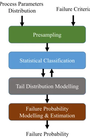
Figure 1.1: Methodology to Estimate Failure Probability of Analog Circuits.

Figure 1.1 shows a simplified block diagram of our methodology. Our methodology falls into the category of statistical classification based methods. The methodol-ogy consists of four processes: (1) presampling; (2) statistical classification; (3) tail distribution modelling; and (4) failure probability modelling and estimation. The inputs to our methodology are distributions of the process variation parameters and circuit specifications defined in term of failure criteria for performance metrics. In the first process, we use LHS and moment matching methods to model the overall performance metric distributions. In the second process, samples that are likely to cause circuit failure are determined using a statistical classifier. In the third process, these likely-to-fail samples are simulated using SPICE and results are modelled as

(24)

tail region of the overall distribution by Generalized Pareto Distribution (GPD) fit-ting. The process of classification and GPD fitting is repeated iteratively to get a better model of tail distribution while reducing sample counts. Finally in the last process, the methodology estimates the rare failure probability of the circuit using the overall distribution and GPD. The output of the methodology is the estimated failure probability.

The proposed methodology estimates the circuit failure probability by analyzing the circuit behavior at the transistor level design. A large analog design with many transistors is not verified as a whole, but is decomposed into blocks. Each sub-block is then further decomposed down to the cell level. A cell is an analog circuit having a certain basic function and the failure probability of the cell is estimated by the proposed methodology.

We also illustrate the application of our proposed methodology on various analog circuits to prove its effectiveness. The circuits used for this purpose, namely, are a ring oscillator, an operational amplifier (opamp) and a Static Random Access Memory (SRAM) cell. We use the opamp and SRAM cell circuits to verify the validity of our methodology to estimate the failure probability of analog circuit in the presence of multiple performance specifications. The ring oscillator circuit is used to verify that our methodology is suitable for high dimensional problems. Our methodology estimates the failure probabilities of all three circuits based on their specifications. We provide an in-depth analysis of obtained results and justify the use of various techniques proposed in our methodology. We also compare the obtained results with other methods, namely, the naive MC method, REscope and Smartera.

1.4 Thesis Contributions

In this thesis, a comprehensive failure probability modeling and estimation method-ology for the analog circuits is presented. The contributions of the thesis can be summarized as follows:

(25)

• We reduced the number of samples required for estimating the failure probability of analog circuits.

• We developed a more practical statistical classifier for analog circuits dataset, which proved to be more efficient and accurate than previously used classifiers for analog circuit failure probability estimation.

• We derived the mathematical formulas to calculate the failure probability in the presence of multiple performance specification and overlapping failure events and developed an algorithm to estimate the probability of overlapping failure events.

• We conducted experiments on three analog circuits to estimate their failure probability in the presence of process variation and multiple performance spec-ification and compared results with other recently published work.

1.5 Thesis Organization

The rest of the thesis is organized as follows: In Chapter 2, we present a brief overview of the concepts and techniques used in this thesis. Then, in Chapter 3, we explain the proposed methodology with an overall flow and detailed description of the sta-tistical classification process developed and mathematical formulation for multiple performance specification. The chapter also describes the algorithm developed for estimating the probability of overlapping failure events due to multiple performance specifications. In Chapter 4, we use the proposed methodology to estimate the fail-ure probability of three test circuits and compare the obtained results with other approaches. Finally, Chapter 5 provides conclusions of this thesis and directions for future research.

(26)

Chapter 2 Preliminaries

In this chapter, we start by giving some basic concepts in probability theory. We briefly describe the notion of Support Vector Machines (SVM) for statistical classifi-cation. Subsequently, we provide an overview of rare event modelling on which our methodology is based. Finally, we present an overview of Latin Hypercube Sampling (LHS), SPICE simulator and k-means clustering which are used in our methodology. The intent of this chapter is to introduce the basic theories and concepts that we use in the rest of this thesis.

2.1 Basic Concepts in Probability Theory

The basic definitions and concepts in probability are briefly reviewed in this section. These concepts are essential for the understanding of statistical failure probability estimation of analog circuits.

2.1.1 Random Variable and Random Process

A random or stochastic variable is a variable (like other mathematical variables) that we cannot say for sure which value it will take on. However, the value that a random variable can take on can be associated with a probability of the value. There are two kinds of random variables: discrete random variables and continuous random

(27)

variables. Adiscreterandomvariablecantakeonvaluesfromaﬁniteorcountably inﬁnitesetofnumbers,e.g.,resultofacointoss. Acontinuousrandomvariablecan takeonvaluesfromanintervalofrealnumbers,e.g.,anyvaluewithintheinterval [0,1]canbeassumedbycontinuousrandomvariable. Normalor Gaussianrandom variablesarethe mostcommonlyencounteredcontinuousrandomvariableinboth manmadeandnaturalphenomena.Processvariationparametersarealsocontinuous randomvariable.

Arandomorstochasticprocessisafunctionthatproducesarandomvariable asanoutput.Itistheprobabilisticcounterpartofadeterministicprocessinwhich outputvaluescanbeknownforsuregiventheinputandinitialconditions.

2 .1

.2 D

istr

ibut

ionFunct

ion

Aprobabilitydistributionisatableoranequationthatlinkseachvalueassumed bytherandomvariableinanexperimentalsettingwithitsprobabilityofoccurrence. Aprobabilitydistributioncanbespeciﬁedinanumberofdiﬀerentways,ofwhich mostcommonaretheProbabilityDistributionFunction(PDF)andtheCumulative DistributionFunction(CDF). Thechoiceofthedistributionfunctionisbasedon mathematicalconvenience.LetX bearandomvariablethatcantakeanyvaluexin theinterval(−∞,∞)withprobabilityPb(x),thentheCDFisgivenby:

F(x)=Pb(X ≤x)=

x

−∞

f(t)dt (2)

CDFisapositiveand monotonicallyincreasingboundedfunctionandF(∞) =1. ThePDFofX isgivenbythefollowingrelation:

f(x)=dF(x)_dx (3)

ThePDFofagaussianrandomvariableisgivenbythefollowingequation:

f(x)=√1

2σ2_πe

−(x µ)2_2σ2 ₍₄₎

(28)

0 0.5 1 1.5 2 2.5 3 3.5 4

x

0 0.1 0.2 0.3 0.4 0.5 0.6 0.7 0.8 0.9 1

f(x)

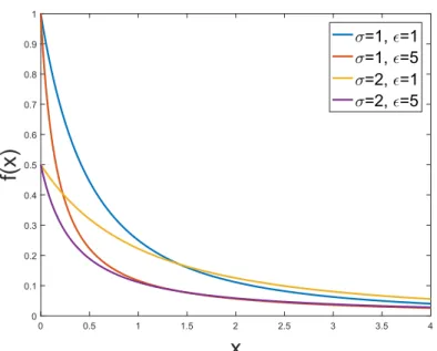
σ=1, ǫ=1 σ=1, ǫ=5 σ=2, ǫ=1 σ=2, ǫ=5

Figure 2.1: Generalized Pareto Distribution for Different Values of σ & , µ= 0.

2.1.3 Generalized Pareto Distribution

The Generalized Pareto Distribution (GPD) is a family of continuous probability distributions often used to model the tails of another distribution. Tail refers to the part of distribution which is quite far away from the mean. GPD allows a continuous range of possible shapes that includes both the exponential and Pareto distributions as special cases. The CDF of GPD is given by the following equation:

F(x) =      1−(1− (x_σ−µ))1 f or 6= 0 1−exp(1− (x_σ−µ)) f or = 0 (5)

where µ is the starting point,σ is the scale parameter, and is the shape paramter. Figure 2.1 shows the CDF of GPD for different values of σ and .

2.2 Support Vector Machines Classifier

A Support Vector Machine (SVM) is a classifier (Section 1.2.4) defined by a hyper-plane separating different categories of data points in the given dataset. A hyperhyper-plane

(29)

is a subspace of one dimension less than its ambient space. We provide an introduc-tory discussion of the basic ideas behind SVMs in this section. SVMs are among the best supervised learning algorithms. By supervised, we mean that SVMs first have to be trained for future predictions.

To explain how the SVM works, we consider a 2-dimensional dataset having two classes/categories of points, as shown in Figure 2.2. The figure also shows multiple lines, separating the two categories. These lines are actually hyperplanes which can be used to categorize new data points. But which is the best among all hyperplanes?

Figure 2.2: Multiple Lines Separating two Classes of 2D Dataset.

A hyperplane is bad if it passes too close to the data points because it will be noise sensitive. Thus the best solution is to find a hyperplane which is as far as possible from data points while still providing a separation between different categories of the data points. The two dotted hyperplanes shown in Figure 2.3 provide the maximum separation between categories. The distance between these hyperplanes is called

(30)

margin. An optimal hyperplane is the hyperplane that lies halfway between the margin. The operation of the SVM algorithm is to search for this optimal hyperplane, that maximizes the margin of the training data.

2.2.1 Linear SVM

The dataset shown in Figures 2.2 and 2.3 can be separated using a linear hyperplane. An SVM classifier that separates different categories of a dataset using linear hy-perplane is called a Linear SVM (L-SVM) classifier. To understand how the linear hyperplane is determined, suppose that we are given a training dataset of n points of the form:

(z~1, y1), ...,(z~n, yn)

Here, yi represents the class of the point z~i, with value either 1 or -1. Each ~zi is a

p-dimensional vector. In this example, a binary classification problem is considered because the classification process adopted in the methodology proposed in this thesis is also binary.

The formal notion to represent a hyperplane is given by the following relation [45]:

~

w.~z−b= 0 (6)

where w~ represents the normal vector to a hyperplane. The parameter _||_wb_|| gives the distance of the hyperplane from the origin in the direction of w~.

If the training dataset is linearly separable (different classes can be separated by a linear hyperplane), the two hyperplanes shown in Figure 2.3, which provide the maximum separation between different categories of dataset are given by the following equations [45]: ~ w.~z−b= 1 and ~ w.~z−b=−1

The distance between these two hypeplanes can be evaluated geometrically, which equals to _||_w2_||. Then to maximize distance between the two classes, ||w|| has to

(31)

be minimized. For mathematical convenience, we state the problem as minimizing

1 2||w||

2_{. Moreover, while minimizing, to prevent data points from falling into the}

margin, we add a constraint to each data point ~zi either

~

w.~zi−b ≥1, ifyi = 1

or

~

w.~zi−b ≤ −1, ifyi =−1

Above mentioned constraint can be rewritten as:

yi(w.~~ zi−b)≥1 , for all 1≤i≤n. (7)

Putting together the problem of minimizing 1₂||w||2 _{and the constraint given in}

Equa-tion 7, we have the following optimizaEqua-tion problem: Minimize 1

2||w||

2

subject toyi(w.~~ zi−b)≥1, for i= 1, ....n

(8)

This is a problem of Lagrangian optimization that can be solved using Lagrange multipliers. It is given by [45]: min L(w) = 1 2||w|| 2₋X i αi yi(w.~~ zi+b)−1 (9)

An important consequence of the geometric description is that the max-margin hy-perplane is determined only by those data points which are nearest to it. These data points are called support vectors. The value of αi in Equation 9 for the datapoint zi

is zero unless zi is a support vector.

The w~ and b that solve the problem given by Equation 9, determine our linear classifier. Given the solution of Equation 9, the decision function of the classifier can be written as:

(32)

2.2.2 Kernel SVM

Evaluating the derivative of Equation 9 with respect to w~ and b and setting them equal to zero, to determine extrema, we have:

~ w=X i αiyiz~i (11) X i αiyi = 0 (12)

Substituting values from Equations 11 and 12 in Equation 9, we get: min L(w) = X i αi − 1 2 X i X j αiαjyiyj(z~i. ~zj) (13)

and substituting values from Equations 11 and 12 in Equation 10, we get:

G(z) =sign(X

i

αiyi(z~i.~z) +b) (14)

From Equations 13 and 14, we determine that the optimization and solution for classi-fication, both depends upon thedot product. If the dataset is not linearly separable in the current feature space, then transforming the feature space into high dimensional space, can make linear separation possible. If the transformed space is given by Φ(~z), then according to Equations 13 and 14, only Φ(z~i).Φ(z~j) and Φ(z~i).Φ(~z) are required

for the training and prediction in the transformed space. Furthermore, if we have a function k(z~i, ~zj) = Φ(~zi).Φ(z~j), the classification can be done in the transformed

feature space without actual transformation. This function is called the kernel func-tion. The kernel function allows SVM to perform non-linear classification. An SVM classifier based on the kernal function is called Kernel SVM (K-SVM). Following two are the most common kernel functions [46]:

• Polynomial: k(z~i, ~zj) = (z~i. ~zj+ 1)d

(33)

2.3 Rare Event Modelling

In Section 1.3, it was stated that the overall distribution of performance metric and its tail region is modelled to estimate rare failure events in our methodology. In this section, we explain how a rare event is modelled and estimated in our methodology Consider an analog circuit with a performance metricY. Because of the variation in manufacturing process, parameters of the test circuit are considered random variables with joint probability distribution S. This in turns makes Y also a random variable since its value depends on parameters values. If our specification requires that any value of Y which is greater than the failure criteria tf causes circuit failure, then the

failure probability P bf of the analog circuit is given by:

P bf =P b(Y > tf) = 1−F(tf) (15)

where F(t) is the CDF of Y. If tf represents some rare event in the distribution of

Y, then P bf represents a rare failure probability. Suppose Y belongs to a Gaussian

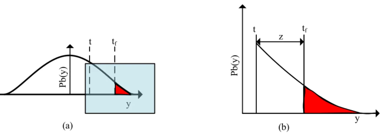
distribution with PDF f(y) given by Equation 4. Suppose t is a threshold that separates the tail from the body of the PDF f(y) and lies between the mean and tf

as shown in Figure 2.4(a), the probability of event Y > t is given by:

P b(Y > t) = 1−F(t) (16)

Let z be an excess over t. Using the concepts of conditional probability [47], the conditional CDF is given by:

F_t0(z) =P b(Y −t≤z|Y > t) = F(z+t)−F(t)

1−F(t) (17)

and the overall CDF as:

F(z+t) = (1−F(t))(F_t0(z)) +F(t) (18) Now if z represents tf −t as shown in Figure 2.4(b), then we have:

(34)

WI W \ 3E \ _3E\ W \ WI ] \ D E

Figure 2.4: Rare Event Modelling using Tail Distribution.

substituting the value of F(tf) given by Equation 19 in Equation 15 and rearranging,

we have:

P bf = (1−F(t))(1−Ft(tf −t)) =P b(t)P b(Y > tf|Y > t) (20)

F

t(tf −t) represents the probability of exceedence and can be modelled by GPD [41]

with µ=t. If Ft(y) represents the CDF of GPD, we have [9]:

P bf =P b(t)P b(Y > tf|Y > t) = (1−F(t))(1−Ft(tf)) (21)

Using Equation 21, we can efficiently estimate the failure probability. F(t) can be accurately estimated using few hundred simulation, using the methods of moment matching (Section 1.2.2). Once estimated, we can model Ft(y) only by simulating

samples in the region Y > t, blocking all other samples. But we do not know which samples of the parameter space when simulated will generate values of the perfor-mance metric Y greater than t. Hence one can employ a statistical classifier to block all samples from being simulated that are unlikely to generate values of Y greater than t. By doing so, an accurate estimation can be made with a small number of simulations. In our methodology t is considered as a relaxed failure criteria while tf

is an actual failure criteria, i.e., the failure criteria given by the designer. Therefore, the classifier is trained on the basis of a relaxed failure.

(35)

While deriving above relation, we assume that the extreme values of interest lie only in the upper tail of the distribution. This is without loss of generality because any lower tail can be converted to the upper tail by replacing y=−y.

2.4 Latin Hypercube Sampling

Latin Hypercube Sampling (LHS) first introduced in 1979, is a sampling method for generating a near-random sample from a multidimensional distribution. In the context of analog circuit verification, LHS is employed for the purpose of variance reduction in the distribution of process variation parameters.

In a 2-dimensional space, a square grid containing sample positions is a Latin square if (and only if) there is only one sample in each row and each column. A Latin hypercube is the generalisation of the concept of Latin square to an arbitrary number of dimensions. When sampling from N variate distribution, LHS partitions the distribution into M intervals of equal probability, and selects one sample from each interval. This forces the number of divisions, M, to be equal for each variable. Moreover, samples for each input are shuffled so that there exists no correlation between the inputs.

2.5 SPICE

Simulation Program with Integrated Circuit Emphasis (SPICE) [19] is powerful gen-eral purpose analog circuit simulator, which is used to predict the circuit behavior and to verify circuit design. SPICE can simulate components ranging from the ba-sic passive elements such as resistors, capacitors and inductors to more sophisticated semiconductor devices such as MOSFETs. Using these intrinsic components as the basic building blocks, very large and complex circuits can be simulated in SPICE. SPICE can perform several types of circuit analysis. Some of the important ones are:

(36)

• Transient analysis • AC analysis • Noise analysis • Sensitivity analysis • Distortion analysis • Fourier analysis • Monte Carlo Analysis

Moreover, using SPICE, the analysis can also be performed for different temperatures. SPICE employs complex transistors and other circuit elements models to predict accurate behaviors.

2.6 k-means Clustering

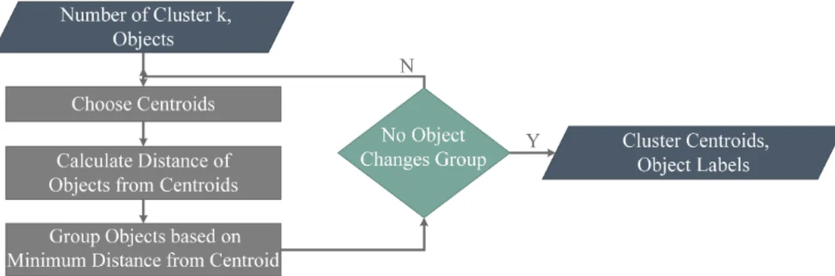
Data clustering is a type of unsupervised learning, that divides a set of objects into groups or cluster in a way that objects of the same group exhibit a certain measure of similarity [45]. One of the most used and popular clustering algorithm is k-means [48]. k-means classifies input objects into predefined number of clusters. Figure 2.5 shows the simplified flowchart of k-means clustering algorithm. The inputs to the algorithm are n objects and a value k that represents the number of clusters. Initially, the algorithm randomly chooses k cluster centroids. For all objects, the distance from each of the centroids is evaluated. The input objects are then assigned to the group associated with the nearest centroid. Based on the members of a group, a new centroid is evaluated for each group. For all objects, the distance from each of the new centroid is evaluated. Based on the minimum distance from new centroids, the membership of the object to a group is then updated. This process is repeated iteratively until no object is reassigned to a new group.

(37)

Figure 2.5: Flowchart of the K-means Clustering Algorithm.

The k-means algorithm requires a low order of memory usage and has a runtime of the order O(n3_{), where n is the number of objects. Moreover, k-means provides}

non deterministic results (different results for different runs) and requires that the number of clusters to be fixed a priori.

2.7 Summary

In this chapter, we discussed some basic concepts in probability theory, namely ran-dom variables, distribution functions, Generalized Pareto Distribution (GPD) and statistics. We then briefly discussed the notion of SVMs for statistical classification. Then, we presented how a rare failure event in analog circuits can be modelled and estimated. Finally, we presented an overview of Latin Hypercube Sampling (LHS), SPICE simulator and the k-means clustering algorithm. The intent of this chapter was to introduce the preliminaries concepts that we will be using in the remaining chapters.

(38)

Chapter 3 Classification and Estimation

Methodology

In Chapter 1, we provided a general overview of the proposed methodology for mod-elling and estimation of analog circuit failure probability and its different processes. This chapter presents a detailed description for each process of the methodology. The methodology consists of four processes and every process is made of different stages. Figure 3.1 shows the proposed methodology processes and their respective stages in the proposed methodology. In this chapter, we explain in dedicated sections every process and all its stages as shown in the figure. We start by describing the first three processes of our methodology, i.e.,presampling,statistical classification and tail distribution modelling. Afterward, we describe the reasons for using an iterative pro-cess of classification and tail modelling and its implementation. Finally, in the last two sections of this chapter, we present the formulation of the failure probability and discuss last process of the proposed methodology, i.e., failure probability modelling and estimation.

To illustrate some of the details of our methodology, we make reference to certain analog circuits, which we use as application case studies in this thesis. A detailed description of the experiments and obtained results on these case studies will be presented in Chapter 4 of this thesis.

(39)

Process Parameters Distribution, Failure Criteria (tf) Initial Sampling Initial Sampling SPICE Simulation SPICE Simulation Distribution Modelling Distribution Modelling

Calculate Relaxed Failure Criteria ( ti )

Explore Likely-Failure-Regions Explore Likely-Failure-Regions

Clustering & Classifier Training Clustering & Classifier Training

Predict Likely-to-Fail Samples Predict Likely-to-Fail Samples

SPICE Simulation SPICE Simulation

GPD Fitting GPD Fitting

No. of iterations = Total percentile bounds

Calculate Probability of

Overlapping Failure EventsCalculate Probability of

Overlapping Failure Events

Model & Estimate Failure Probability Model & Estimate Failure Probability

Failure Probability Percentile Bounds b={ b1, b2, b n } N Y Presampling Statistical Classification Tail Distribution Modelling Failure Probability Modelling & Estimation

Process Input

Stage

Iteration Control Output

(40)

3.1 Presampling

The first process of our methodology is presampling. The purpose of presampling is to sketch the approximate behavior of the analog circuit. The output from the presampling stage is later used for classifier training. Presampling itself consists of three phases:

Initial Sampling

At this point of the methodology, we are only interested in observing the circuit’s approximate behavior that can be achieved using a few hundred samples of pro-cess variation parameters [43]. If the distribution of n process variation parameters

p1, p2, ...pn is given by S = {P1, P2, ...Pn}. Then in order to model the PDF of the

performance metrics and later for the initial classifier training, a few hundred sam-ples, _S={s0, s1, ...sm} are drawn fromS. Where si ={p1,i, p2,i, ....pn,i} and m is the

total number of samples drawn. Each element of _Srepresents the set of values of the parameters for the circuit. This process of sampling is performed at the beginning of the methodology and is known as Initial Sampling. Samples are drawn using LHS.

Circuit Simulation

Initial Sampling provided samples _S as output. The second phase of presampling deals with evaluating the value of performance metric Y of the circuit for the pro-cess parameters samples _S. This is achieved by performing a transistor level SPICE simulation on every sample of the set _S. SPICE simulations yield y0, y1, ...ym as the

values of Y corresponding to the samples s0, s1, ...sm, respectively.

Distribution Modelling

Due to process variation,Y also follows a probabilistic distribution. At this point, the PDFf(y) ofY is approximated to an analytical form using the results obtained from

(41)

Figure 3.2: PDF Approximated using LHS and MC.

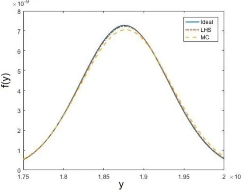
circuit simulation phase. A conventional way of fitting the PDF to an approximate analytical form is by applying moment matching methods (Section 1.2.2) on a small set of naive MC samples. In our methodology, we use samples drawn using LHS to approximate the PDF to an analytical form. Samples are more evenly spread across all possible values by the use of LHS. This helps in better PDF fitting with a smaller number of samples as compared to samples selected using the naive MC method. Figure 3.2 shows the sketches of PDF modelled using samples drawn by LHS and naive MC.

500 sample were drawn using LHS and naive MC to model the PDF of the output frequency of a ring oscillator circuit, subject to process variations of 30 parameters. Figure 3.1 clearly illustrates the advantage of using LHS for PDF fitting compared to naive MC. LHS provides a better accuracy with a smaller number of samples hence resulting in a speedup.

(42)

behavior off(y) and accuracy of the moment matching method used for approximat-ing it. The value of t is such that, F(t) can be accurately estimated and t lies in between the nominal value ynom and the actual failure criteriatf, in the distribution

of Y, whereF(y) is the CDF of Y. The process of determining the value oft will be discussed later in this chapter.

3.2 Statistical Classification

In this process of our methodology, a classifier model is used to categorize a sample

so as likely-to-fail or unlikely-to-fail. Therefore, we can skip the unlikely-to-fail

sam-ples and focus only on likely-to-fail ones. Likely-to-fail samsam-ples belong to a single or multiple regions in parameters space called Likely-to-Fail Regions (LFRs). Any sam-ple drawn from LFR when simulated is more likely to cause circuit failure. Similarly, unlikely-to-fail samples are members of a single joint Unlikely-to-Fail Region (ULFR), which are unlikely to cause circuit failure. In this section, we first provide some back-ground to classifiers used in other approaches and also discuss their limitations. Then, we provide details of a new classifier model developed for our methodology.

3.2.1 Background

The authors of the Statistical Blockade (SB) [42] and Recursive Statistical Block-ade (RSB) [27] approaches proposed to use linear SVM (L-SVM) classifier. While in REscope [43] and Smartera [44] approaches, use of a Gaussian Radial Basis Function (GRBF) based kernel SVM (K-SVM) classifier is proposed for non-linear classifica-tion. As discussed in Section 2.2, SVMs either operate unequivocally in the input feature space giving rise to L-SVM or by using kernel mapping of feature space to higher dimensions, leading to K-SVM. L-SVM only uses dot product operation, there-fore they are simple to train and use. However, they cannot be applied on non-linear data. K-SVM on other the hand can tackle the dataset which is not linearly separa-ble. However, K-SVM is not as efficient as L-SVM. Moreover, GRBF based K-SVM

(43)

Figure 3.3: Effects of Kernel Scale γ on the GRBF based K-SVM classifier: (a) Reference Data; (b) γ = 1; (c)γ = 10; (d) γ = 100.

requires the setting of a parameter called kernel scale γ. For a lower value of γ, K-SVM is unable to capture the non-linear behavior of the boundary separating classes. While setting a higher value of γ forces K-SVM training algorithm to try harder to avoid misclassification which can consequently result in overfitting. Overfitting can significantly reduce classification accuracy. Figure 3.3 shows the effect ofγ on classi-fication accuracy of the GRBF based K-SVM classifier when used to determine LFRs of a ring oscillator circuit in the presence of two process parameters. The red region in Figure 3.3(a) represents the realistic failure region while the red region in Figures 3.3(b)-(d) represents LFR determined by the K-SVM classifier.

Based on the above discussion, it is desirable to have a classifier model which has the simplicity and efficiency of an L-SVM classifier and the high discriminative power

(44)

of a non-linear classifier such as a K-SVM classifier. The authors of [49] proposed the idea of using multiple L-SVM classifiers for non-linear classification. The authors of [49] used a mixture model of L-SVM classifiers. The approach is based on partitioning the input space (or feature space) into hyperspherical regions, in which the data is linearly separable. Experiments performed on synthetic and real world applications indicated a better training time of all L-SVM classifiers combined, with the accuracy equal to that of non-linear classifiers. This idea of using multiple L-SVM classifiers was further extended by the authors of [50, 51, 52]. All of these work employed a complex model for partitioning the feature space to make their method general in nature. These complex methods added computational cost.

In our methodology, we also propose the use of multiple L-SVM classifiers instead of a single non-linear classifier. But since our applications of statistical classification only focus on the failure probability estimation of analog circuits, assumptions can be made about the dataset. With these assumptions, complex models for partitioning a feature space are avoided and a rather simple method is adopted with significantly less computational cost. Following assumptions are drawn:

• Classification problem is binary in nature i.e. either unfail or likely-to-fail.

• A single ULFR exists in the feature space.

• Unlikely-to-fail samples may only be concentrated around edges of the feature space.

These assumptions were drawn by observing the behavior of different analog circuits in the presence of process variations. Based on these assumptions, we propose a classification approach in which the dataset is divided into multiple clusters. Each cluster contains both unlikely-to-fail and likely-to-fail samples which are almost lin-early separable. Moreover, the unlikely-to-fail or likely-to-fail status of the training sample is evaluated based on t, the relaxed failure criteria. In remaining parts of

(45)

this section, we describe how the classifier model is developed and its working in the overall methodology.

3.2.2 Algorithm Overview

Figure 3.4: L-SVM Classification Results in the Presence of Multiple Failure Regions: (a) Reference Data; (b) Predicted Results.

A single L-SVM classifier can only linearly separate a dataset. When there ex-ist multiple LFRs in the process parameter space, unlikely-to-fail and likely-to-fail samples cannot be separated using a single linear hyperplane. Hence, when a single L-SVM is used in this case, it fails completely. Figure 3.4 shows the classification accuracy of a single L-SVM classifier when used to categorize samples of a ring os-cillator circuit in the presence of two process parameters and multiple LFRs. The red points in Figure 3.4(a) indicate samples of process parameters which generate a circuit behavior not meeting the desired specification, while the blue points represent samples generating the desired circuit behavior. It can also be seen from Figure 3.4(a) that there exist two LFRs in the parameters space. However, the red points in Figure 3.4(b) represent samples categorized likely-to-fail by the L-SVM classifier, while the blue points represent samples categorized as unlikely-to-fail. When the results pre-sented in both Figures 3.4 (a) and (b) are compared, it can be seen that the L-SVM classifier categorized most of the failing samples as unlikely-to-fail, indicating a very

(46)

low classification accuracy.

To overcome this problem, in the first stage of our classification process, LFRs are explored. In the next stage, considering one LFR at a time, a clustering scheme is applied. In doing so, we avoid the problem of having multiple LFRs in a single cluster. Once the clusters are evaluated, multiple L-SVM classifiers are trained. Finally, in the last stage, samples are drawn and categorized as either to be unlikely-to-fail or likely-to-fail.

3.2.3 Exploring LRFs

In the first step of our classification process, LFRs are explored based on the approach proposed in [38]. LFRs represent rare events in the distribution of the performance metricY. To effectively explore all LFRs, a large number of samples have to be drawn from the distribution of process parameters S and simulated. A surrogate model is used to overcome this problem in [38], which maps a sample s fromS to the value y

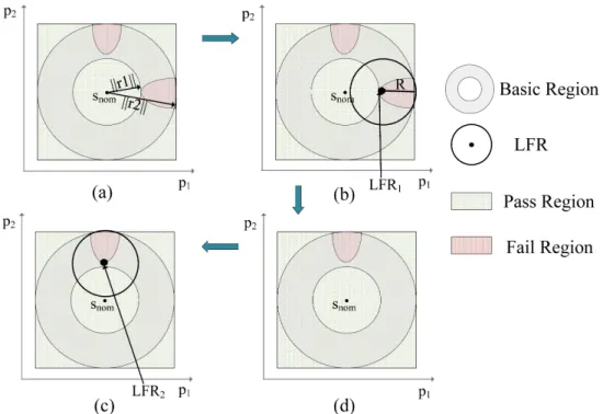
of the metric Y. The predicted y, obtained from the model, was then used for LFRs exploration. This approach proved useful in low dimension but failed completely in high dimensions. In our methodology, a relaxed failure criteria is chosen, hence making LFRs less rare events. Therefore, LFRs can be explored effectively with only a few hundred samples_S, simulated during the presampling stage. LFRs are explored in two stages. Figure 3.5 shows the complete procedure for exploring LFRs.

1) Basic Region Definition

A basic region represents the sub-region in the parameters space where LFRs will be explored. In Figure 3.5(a) it is the region within the two hypershperes of radius of ||r1|| and ||r2|| with common center snom. Where snom is the nominal value of the

process parameters and ||•|| isL

2-norm function [30]. r1 is given by:

(47)

Figure 3.5: Procedure to Explore LFRs: (a) Basic Region Definition; (b) Explore First LFR; (c) Explore Second LFR; (d) Remove First.

where sr1 represents a sample causing circuit failure and it lies closest to snom in the

space defined by S. Once||r1|| is evaluated, ||r2||is determined, and is given by:

r2 = sr2−snom (23)

where sr2 represents a sample causing circuit failure and it lies furthest away from snom.

2) LFRs Exploration

The goal of this stage is to determine the number of LFRs,x, in the basic region. To do so, only the samples residing in the basic region are selected for LFRs exploration. As shown in Figure 3.5(b), a hypercube with center sr1 and radius R=||r1|| − ||r2||

is defined. Samples of the basic region causing circuit failure and lying within this hypercube are selected and the first LFR is determined. The selected samples are then removed from the basic region (Figure 3.5(d)). A new sr1 is then determined

(48)

Figure 3.6: Special Condition in LFR Exploration.

from the remaining samples of the basic regions. The new value ofsr1 is then used to

define another hypercube which is shown in Figure 3.5(d). Samples that lie within the hypercube shown in Figure 3.5(c) are then selected and the second LFR is determined. This process goes on until there exist no such sample in the basic region that causes circuit failure. After that, the k-means algorithm is applied to divide all samples causing circuit failure intox groups. The output of the k-means algorithm includesx

group (LFR) means and labels indicating the membership of input samples to their respective LFR.

Figure 3.6 shows a special condition which may arise during the LFR exploration. The realistic failure region is larger so that the LFR does not completely contain it. When this condition happens, the realistic failure region will be treated as several failure regions, and the other part (the yellow line in Figure 3.6) will be explored in the next iteration stage. As a result, the number of LFRs determined will be more than the number of realistic failure regions in the parameter space. The k-means algorithm is applied multiple times to overcome this problem. The k-k-means algorithm will provide significantly different means for different runs when the value of x is more than the number of realistic failure regions. If this situation arises, the

(49)

Algorithm 3.1 Exploring LFRs.

Require: _S,Z,snom

1: sr1, ||r1||, sr2, ||r2||

= Basic Region P aramters(_S, Z, snom)

2: _S0, Z0 = Basic Region Sample(_S,||r1||,||r2||, snom)

3: R = ||r1|| − ||r2||

4: repeat

5: x = x + 1

6: _S0, Z0 =Explore LF R(_S0, Z0, R, sr1) 7: sr1 =Basic Region P aramters(S0, Z0, snom)

8: until sr1 6= null

9: _S_{F ail} = samples causing circuit failure

10: repeat 11: [S1,LF R, U1] = kmeans(SF ail, x) 12: [S2,LF R, U2] = kmeans(SF ail, x) 13: [S2,LF R, U3] = kmeans(SF ail, x) 14: if S1,LF R∼=S2,LF R ∼=S2,LF R then 15: Stop = 1 16: SLF R = S2,LF R; U =U1 17: else 18: x =x -1 19: end if 20: until Stop 6= 1 21: return x, SLF R, SF ail, U

value of x is decreased by one and the k-means algorithm is applied multiple times using the updated value of x. This process is repeated until the means, determined by applying the k-means algorithm multiple times, are almost the same.

Implementation

A simplified implementation of the complete procedure to explore LFRs, is given in Algorithm 3.1. The inputs to the algorithm are following:

• Samples of parameters space, _S={s1, s2, ..sm}

• Category labels, Z = {z1, z2, ...zm}. The value of zo can either be 1 or 0 for

the sample so. A 0 value indicates thatso causes circuit failure while a 1 value

(50)

• The nominal value of the process parameters, snom.

In Line 1, the algorithm outputs sr1, ||r1||, sr2 and ||r2|| using the function Basic Region P aramter(). The inputs to the function Basic Region P aramter() includes _S, Z and snom. The function Basic Region P aramters() evaluates the

dis-tance of every sample in _Sfrom snom and determines the samples sr1 and sr2

accord-ingly. The function then evaluates||r1||and||r2||. In Line 2, the algorithm determines the samples residing in the basic region using the function Basic Region Sample(). The input to the functionBasic Region Sample() includes _S, snom and the

parame-ters of the basic region determined in Line 1. The output of the function is a group of samples _S0 and their respective category labels Z0. The distance of any sample, in the group _S0, from snom is between the interval

||r1||,||r2||

. From Lines 3-8, the number of LFRs x is determined. The function Explore LF R() in Line 6 removes those samples from the basic region that causes circuit failure and lie in the region defined by hypercube with the center snom and radius R. In Line 7, a new value

of sr1 is determined from the remaining samples of the basic region by using the Basic Region P aramter() function. Each time a new value ofsr1 is determined, the

value of xis incremented by one.

After that, the algorithm from Lines 10 to 20 iteratively determines the cor-rect value of x by applying the k-means algorithm multiple times. Finally, the al-gorithm converges when a correct value of x is determined and provides the out-put in Line 21. The output of the algorithm includes x, LFR means SLF R =

{SLF R−1, SLF R−2, ...SLF R−x}, the samples SF ail causing circuit failure and their

la-bels U, indicating the LFR to which they belong.

3.2.4 Clustering & Classifier Training

After the LFRs exploration stage, we move forward with the objective of clustering our feature space. We perform the clustering considering one LFR at a time. If the boundary between the LFR and ULFR is considered as a non-linear curve, dividing this curve into small segments results into portions of curves which are approximately

(51)

Figure 3.7: Piecewise Linearization of a Non-Linear Curve

linear. This principle is adopted in our clustering scheme. Figure 3.7 shows the principle of piecewise linearization of a non-linear curve (failure boundary) used in our classifier model. A hyperplane is determined whose direction is parallel to the curve’s tangent shown in the figure. Multiple hyperplanes are then determined which are normal to the previously determined hyperplane. These hyperplanes are directed inwards the non-linear curve. If there are enough of these normal hyperplanes, a segment of the non-linear curve, lying between any two normal hyperplanes, can be considered approximately linear.

1) Cluster Centroid Evaluation

The first step, to cluster the input space defined by S, is to evaluate the centroid for each cluster. Centroids are evaluated using Algorithm 3.2. The inputs to the algorithm are following:

(52)

Algorithm 3.2 Clusters Centroids Evaluation. Require: x,_S, snom, SLF R,U 1: [G0, G2, ...Gx] = Group(S, U) 2: for i=1 to x do 3: l =Calc Distance(sLF R−i, Gi) 4: α = (snom−sLF R−i)/2 5: A = {G0∪Gi} 6: k = number of samples inA 7: for j=1 to k do 8: d1 =||snom−aj|| 9: d2 =||sLF R−i −aj|| 10: d3 =||α−aj||

11: wj =F ind(min(D)) .where D={d1, d2, d3}

12: end for 13: J =F ind(W == 3) . where W ={w1, w2, ..wk} 14: B0 =Assign(A,J) 15: J =F ind(||α−B0|| ≤l) 16: B = Assign(B0,J) 17: Ci =kmeans(B, β) 18: C = C ∪ Ci 19: end for 20: return C

• Samples of the parameters space, _S={s1, s2, ....sm}.

• Sample snom, representing nominal values of the process parameters.

• LFRs Means, SLF R ={sLF R−1, sLF R−2, ...sLF R−x}

• LFRs label, U ={u1, u2, ...um}. u can take any integer value between 0 andx.

A 0 value ofu indicates that a samples belongs to ULFR. Any other value iof

u indicates that a samples belongs toith LFR with mean given by sLF R−i.

In Line 1, the algorithm output G1, G2, ..Gx that represents the group of samples

having a common label defined by U. Moreover, G0 represents the group of samples

belonging to ULFR while all other groupsG2, ..Gxcontain samples of respective LFR.

From Lines 2 to 19, the centroids C ={c1, c2, ...c(β∗x)} are determined. β represents

the number of clusters per LFR. The centroids are determined considering one LFR at a time. In Line 3, using the function Calc Distance(), the algorithm outputs l

Statistical Classification Based Modelling and Estimation of Analog Circuits Failure Probability

Statistical Classification Based Modelling and Estimation of

Analog Circuits Failure Probability

Muhammad Shirjeel Shehzad

&21&25',$81,9(56,7<

6FKRRORI*UDGXDWH6WXGLHV

Abstract

Statistical Classification Based Modelling and Estimation of Analog

Circuits Failure Probability

Muhammad Shirjeel Shehzad

Acknowledgments

Contents

List of Figures

List of Tables

List of Acronyms

Chapter 1

Introduction

1.1

Motivation

1.2

Related Work

1.2.1

Monte Carlo and its Variants

1.2.2

Moment Matching

1.2.3

Importance Sampling

1.2.4

Statistical Classification Based Methods

1.3

Proposed Methodology

1.4

Thesis Contributions

1.5

Thesis Organization

Chapter 2

Preliminaries

2.1

Basic Concepts in Probability Theory

2.1.1

Random Variable and Random Process

2

.1

.2 D

istr

ibut

ionFunct

ion

x

f(x)

2.1.3

Generalized Pareto Distribution

2.2

Support Vector Machines Classifier

2.2.1

Linear SVM

2.2.2

Kernel SVM

2.3

Rare Event Modelling

2.4

Latin Hypercube Sampling

2.5

SPICE

2.6

k-means Clustering

2.7

Summary

Chapter 3

Classification and Estimation

Methodology

3.1

Presampling

Initial Sampling

Circuit Simulation

Distribution Modelling

3.2

Statistical Classification

3.2.1

Background