Pricing Python Parallelism: A Dynamic Language Cost Model for Heterogeneous Platforms

Jacob, D., Trinder, P. and Singer, J. (2020) Pricing Python Parallelism: A Dynamic

Language Cost Model for Heterogeneous Platforms. In: 16th ACM SIGPLAN

International Symposium on Dynamic Languages, Virtual, USA, 17 Nov 2020, pp.

29-42. ISBN 9781450381758 (doi:

10.1145/3426422.3426979

).

There may be differences between this version and the published version. You are

advised to consult the publisher’s version if you wish to cite from it.

© Association for Computing Machinery 2020. This is the author's version of the

work. It is posted here for your personal use. Not for redistribution. The definitive

Version of Record was published in Proceedings of the 16th ACM SIGPLAN

International Symposium on Dynamic Languages, Virtual, USA, 17 Nov 2020, pp.

29-42. ISBN 9781450381758.

http://eprints.gla.ac.uk/226320/

Deposited on: 20 November 2020

Enlighten – Research publications by members of the University of Glasgow

http://eprints.gla.ac.uk

Pricing Python Parallelism: A Dynamic Language

Cost Model for Heterogeneous Platforms

Dejice Jacob

Phil Trinder

Jeremy Singer

Abstract

Execution times may be reduced by offloading parallel loop nests to a GPU. Auto-parallelizing compilers are common for static languages, often using a cost model to determine when the GPU execution speed will outweigh the offload overheads. Nowadays scientific software is increasingly writ-ten in dynamic languages and would benefit from compute accelerators. The ALPyNA framework analyses moderately complex Python loop nests and automatically JIT compiles code for heterogeneous CPU and GPU architectures.

We present the first analytical cost model for auto-parallelizing loop nests in a dynamic language on heterogeneous architec-tures. Predicting execution time in a language like Python is extremely challenging, since aspects like the element types, size of the iteration space, and amenability to parallelization can only be determined at runtime. Hence the cost model must be both staged, to combine compile and run-time in-formation, and lightweight to minimize runtime overhead. GPU execution time prediction must account for factors like data transfer, block-structured execution, and starvation.

We show that a comparatively simple, staged analytical model can accurately determine during execution when it is profitable to offload a loop nest. We evaluate our model on three heterogeneous platforms across 360 experiments with 12 loop-intensive Python benchmark programs. The results show small misprediction intervals and a mean slowdown of just 13.6%, relative to the optimal (oracular) offload strategy.

CCS Concepts:• Software and its engineering→

Dy-namic compilers;Just-in-time compilers; •Computer

sys-tems organization→Heterogeneous (hybrid) systems.

Keywords:nested loop parallelization, cost model, Python,

GPU

ACM Reference Format:

Dejice Jacob, Phil Trinder, and Jeremy Singer. 2020. Pricing Python Parallelism: A Dynamic Language Cost Model for Heterogeneous DLS ’20, November 17, 2020, Virtual, USA

© 2020 Association for Computing Machinery.

This is the author’s version of the work. It is posted here for your personal use. Not for redistribution. The definitive Version of Record was published in

Proceedings of the 16th ACM SIGPLAN International Symposium on Dynamic Languages (DLS ’20), November 17, 2020, Virtual, USA,https://doi.org/10. 1145/3426422.3426979.

Platforms. InProceedings of the 16th ACM SIGPLAN International Symposium on Dynamic Languages (DLS ’20), November 17, 2020, Virtual, USA.ACM, New York, NY, USA,14pages.https://doi.org/ 10.1145/3426422.3426979

1

Introduction

Dynamic scripting languages like Python are increasingly popular, particularly for domain-specific scientific code writ-ten by end users. Meanwhile compute accelerators, such as GPUs, are increasingly available on commodity devices at all scales. Much recent research effort has focused on identifying parallelism in such end user programs and ex-ploiting this parallel code on manycore hardware. Different approaches include embedding domain-specific parallel code

in dynamic languages [20,21] or using parallel APIs,

pat-terns and libraries [8,11]. However, there has been little

focus on theautomaticselective application of such

paral-lel optimizations. In prior work, coders are left to choose manually which sections of their program should be paral-lelized. Such techniques rely on the risky assumption that the programmer knows best.

Rather than require that developers have parallel program-ming expertise, our approach is to automatically parallelize loop nests in vanilla Python on GPUs. The ALPyNA frame-work has demonstrated significant reduction in runtimes of

large and moderately complex loop nests [14,15] (Section2).

However offload overheads like kernel compilation and data transfer mean that offloading small loops is slower than CPU execution.

The key technical contribution of this paper is a new pa-rameterized, lightweight and staged cost model, the ALPyNA

Cost Model (ACM), thatautomaticallyand selectively applies

loop parallelization to minimize runtime (Section3). This is

precisely what non-expert scripting programmers require on current commodity platforms with multiple heterogeneous compute resources.

While cost models for automatic compilation and

paral-lelization are common for static languages (Section6),

mod-elling a dynamic language like Python poses significant chal-lenges. Parallelizing compilers for static languages have far more program information, can use profiling or heavyweight offline analysis, and may speculatively generate code for al-ternative execution platforms. Such techniques are severely restricted in dynamic language implementations as so much

program information is determined only at runtime. For example the parallel structure of a Python loop nest can only be determined dynamically when iteration domains are dynamic, and dependences cannot be resolved statically. Moreover in a dynamically typed language the array element types are dynamic, and these determine costs like GPU data transfer times.

Fortunately modern sophisticated dynamic language im-plementations now provide the technologies to address auto-parallelization challenges. For example the dynamically de-termined safe loop nest can be JIT compiled for CPU or GPU; likewise runtime introspection allows dynamic type informa-tion to be extracted and used to parameterise the cost model.

To the best of our knowledge ACM isthe first analytical

cost model that supports the automatic runtime exploitation of GPUs in a dynamic language.

For each instance of a loop nest, ACM dynamically pre-dicts the relative runtimes on alternative execution platforms so that ALPyNA can select the fastest. ACM is staged, com-bining compile-time analysis with runtime introspection in the CPython interpreter to parameterise the static model. The model is designed to be lightweight as it is evaluated at runtime. The ACM models for interpreted and JIT-compiled CPU execution are simple and relatively standard. In con-trast the GPU model is both elaborate and more novel as it accounts for key device costs, including the time to trans-fer data to and from the device, block structured execution, starvation effects etc. All of the platform models are paramet-ric in key characteristics of the devices in a heterogeneous platform, like warp size on the GPU.

An important scientific contribution is to show that a comparatively simple staged analytical model can effectively determine at runtime whether to offload a loop nest in a

dynamic language (Section5). Comparatively simple cost

models for the parallel platforms suffice because the system

does not attempt to accurately predictabsoluteloop runtimes,

rather it compares therelativeruntimes on the GPU and

CPU with interpretation or JIT compilation. Of course such relative cost models are common for static languages (Section

6).

2

Parallelizing Python Loops with

ALPyNA

ALPyNA is an auto-parallelizing framework for heteroge-neous architectures that parallelizes dense linear loop nests

written in vanilla Python [14,15]. Linear loop nests consist

of statements in which array subscripts are linear expres-sions of the loop iterator variables. While the examples below are very simple, ALPyNA can analyze loop nests that are

moderately complex: the benchmarks in Section5

demon-strate ALPyNA parallelizing multiple loops in a program, nested loops, perfect and imperfect loop nests, and nests with control flow divergence.

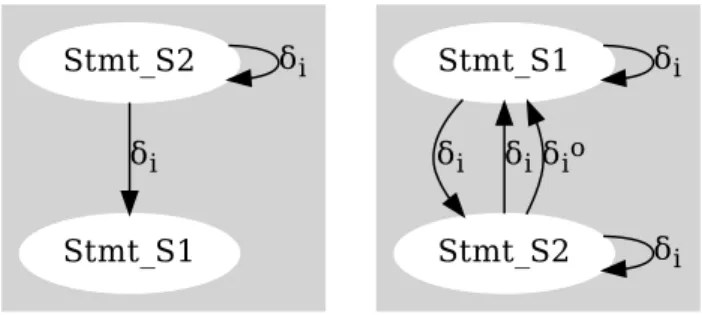
Stmt_S1 Stmt_S2

δ_i

δ_i

Figure 1. Dependence graph

for Listing1loop nest with it-eration domain (i,j)←(32,1024) and (k)←64

Stmt_S1 δ_i

Stmt_S2

δ_i δ_iδ_io

δ_i

Figure 2. Dependence graph

for Listing1loop nest with it-eration domain (i,j)←(32,1024) and (k)←(8)

2.1 Runtime Dependence Analysis

ALPyNA parallelization relies on analyzing the dependence relationships between variables in the loop nests, as

popu-larised by Allen and Kennedy [18] for FORTRAN. The

de-pendence analysis uses standard techniques to solve systems

of linear equations [38] determined by loop domain limits

and array subscripts. When these domains are unknown at compile time, a static compiler must conservatively assume that dependences exist.

For simple loop nests, optimizing static compilers try and create parallel and sequential variants. Execution of such speculatively generated parallel variants is subject to guard conditions being satisfied. Such systems, like MegaGuards

(Qunaibit et al[30]), are available for interpreted languages

like Python. However, generating multiple variants of loop nests based on different combinations of dependence rela-tionships quickly becomes unwieldy even if only a small number of factors are unknown at compile time.

def l n _ f u n c ( a r g _ a , k , l i m i t s ) : im , jm = l i m i t s for i in ran ge( 0 , im , 1 ) : for j in ran ge( 0 , jm , 1 ) : # S t a t e m e n t − S 1 a r g _ a [ i +k , j ] = a r g _ a [ i , j ] + 4 # S t a t e m e n t − S 2 a r g _ a [ i + 1 6 , j ] = a r g _ a [ i , j ]

Listing 1.ALPyNA loop nest parallelization example

Consider the loop nest in Listing1. The dependence

re-lationships between the two statementsS1andS2is

deter-mined by loop bounds(im,jm), the loop invariant variable

‘k’ and the coefficients and constants in each array subscript.

Due to the unresolved loop domain sizes and non-iterator

variable within the array subscript on the LHS ofS1, a purely

static compiler must conservatively generate sequential code.

Figure1shows the dependence graph for an instance of the

and(k) ← (64). All 32×1024 execution instances of

State-mentS1can safely be executed in parallel becausek>im.

For statementS2, executing the outer loop(F_i)sequentially

allows 1024 execution instances (corresponding to the inner

loopF_j) to be executed in parallel. Figure2shows the

de-pendence graph for the same loop nest with domain limits

(im,jm) ← (32,1024)and variable(k) ← (8). Ask<imthe

inner loop(Fj)may only be executed in parallel if the outer

loop(Fi)is executed sequentially. If the loop limits have the

values(im,jm) ← (16,1024)and(k) ← (16), all instances of

statementsS1andS2can be executed in parallel.

Primary contributions in this paper are the development of a hybrid cost model that estimates the relative execution time of such loops, and the integration of this cost model

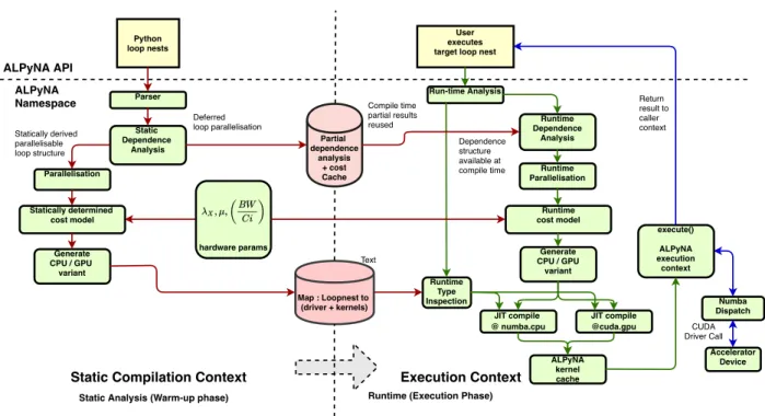
into the ALPyNA system (Figure3).

2.2 ALPyNA System Architecture

ALPyNA is not a whole program compiler: users invoke loop analysis by passing marked functions with loop nests in them to the system. ALPyNA isolates and analyzes these loops and either JIT compiles for the CPU or generates GPU kernels and schedules them while preserving dependence relationships. Any Python statements between loop nests are executed within the interpreter. It first parses loop nests and performs loop normalization (i.e. transforms loops to increment by unit stride) to facilitate dependence analysis. Control flow divergence within loop nests is handled by con-verting computational statements to predicated statements

usingif-conversion. ALPyNA allows calls topure intrinsic

functions within the loop body to aid computation. These are mapped onto corresponding intrinsics supplied by the

Numba compiler (Section2.3) for a particular target device.

A loop nest with computation that cannot be JIT compiled by Numba is executed by the interpreter.

Figure3provides an overview of ALPyNA’s architecture,

incorporating the cost model extensions. The parser gen-erates a very simple flat record structure of the loop nests which are grouped into ‘loop landmarks’. Any loop limits that cannot be statically determined are marked for runtime analysis. The presence of variables within array subscripts which are not loop iterators are also marked for runtime analysis.

If all dependence relationships can be determined at com-pile time, skeletal kernels and drivers are generated and cached. During runtime, when the loop nest is invoked, ALPyNA introspects the data types of the data being ac-cessed within the loop nest and determines the types to be patched into the skeletal kernels that have been generated. These kernels are then compiled using Numba.

If a dependence relationship cannot be ascertained at com-pile time, any dependence that can be statically derived is memoized and the whole loop nest is marked for runtime analysis and optimization. At runtime, ALPyNA intercepts

invocations of these loop nests. All relationships deferred to runtime analysis are computed for each loop nest instance. In the presence of unknown loop limits and other variables (such as loop invariants), a static compiler would have to be conservative and assume that dependences exist. In contrast ALPyNA uses introspection to determine loop domain limits and other variable relationships at runtime to aggressively exploit potential parallelism. ALPyNA combines statically derived dependences and those determined at runtime to compute the overall dependence relationships in a loop nest. The loop nest is then converted into a skeletal form to pass into the code generator for each target architecture. After the loop nest has been analyzed and transformed into a skeletal structure, code is custom generated for the depen-dence relationships that exist for an execution instance of the loop nest. Code generated by ALPyNA after dependence

analysis is JIT compiled using Numba (Section2.3).

2.3 Numba Compiler

ALPyNA uses the Numba [23] library to JIT compile and

execute loop nests. Numba is an LLVM based framework that can dynamically compile Python functions. Normally,

programmers add a @jit decorator to a Python function

to compile it to CPU machine code. Numba also has the

@cuda.jitdecorator syntax to provide access to CUDA

bind-ings. This enables programmers to write CUDA kernels for GPU using restricted Python semantics and CUDA idioms.

For ALPyNA, developers provide undecorated Python source code. After staged analysis/parallelization passes, ALPyNA will eventually invoke Numba to JIT compile syn-thesized Python code for the appropriate backend target de-vice (CPU or GPU). Our new cost model (ACM) is intended to guide the dynamic selection of target devices.

Numba compiles code at runtime once the concrete data types of the variables within the code are determined. While automatic type inference is provided within Numba, the cost of compiling and type-checking is expensive. Numba allows programmers to optionally specify data types within the

@[email protected]. A compiled kernel is cached

to reduce execution time. Since ALPyNA generates a GPU kernel for each statement, each loop invocation of a GPU kernel (caused by sequential execution of a loop to maintain a loop-carried dependence) would trigger automatic type-inspection by Numba. This reduces performance by an order of magnitude, and to ameliorate this ALPyNA performs type inspection and supplies each kernel with the requisite types. This enables Numba to re-use a previously cached kernel without fresh type inspection.

2.4 GPGPU Programming Model

Current NVIDIA GPU architectures execute parallel threads

on parallel cores called a Streaming Multiprocessor (SM) [12].

Each SM has a large number of CUDA cores and potentially

Parser Python loop nests Static Dependence Analysis Parallelisation Statically derived parallelisable loop structure ALPyNA API

Static Analysis (Warm-up phase) Runtime (Execution Phase)

User executes target loop nest

ALPyNA Namespace Run-time Analysis Runtime Type Inspection Runtime Parallelisation Dependence structure available at compile time

Static Compilation Context Execution Context

Deferred loop parallelisation execute() ALPyNA execution context Return result to caller context Runtime Dependence Analysis Compile time partial results reused ALPyNA kernel cache Numba Dispatch CUDA Driver Call   Accelerator Device Partial dependence analysis + cost Cache   hardware params Statically determined cost model Generate CPU / GPU variant Runtime cost model Generate CPU / GPU variant JIT compile @cuda.gpu JIT compile @ numba.cpu Map : Loopnest to (driver + kernels) Text

Figure 3.Overall system architecture, showing how when dependences cannot be determined statically, we defer dependence

analysis to runtime, when kernels can be specialised to runtime dependences and domain sizes.

threads for execution on awarpsized subset of CUDA cores

in an SM. Every thread within a warp executes an instruction in lock-step on CUDA cores. An SM may also have a number

of shared caches [33].

This model is abstracted for the programmer as compu-tational kernels executed in parallel on a GPU. An instance

of kernel execution is identified with athreadIdand threads

are arranged into a threadblock. The number of threads in a threadblock are limited, e.g. to 1024. The number of threads executing instances of a kernel can be increased

by executinggridsof equal-sized thread blocks. In CUDA,

threads are logically arranged along one, two, or three di-mensional axes in a two tier structure of grids and blocks

[12,26]. The actual threadId along a particular axis can be

dereferenced using simple two tier dereferencing seman-tics(blockidaxis×blocksizeaxis+threadIdaxis). The three axis

thread hierarchy(x,y,z)of GPGPU programming originate

from 3D graphics computation. Parallel threads in a thread

block are expected to be scheduled on the same SM [12].

Dependence theory states that if a dependence in a loop

nest iscarried by a loop, executing this loop sequentially

allows any nested loops to be executed in parallel, so long as

they do not carry any other loop dependences [18]. ALPyNA

uses dependence analysis to parallelize such inner loops. It generates a single GPU kernel for each loop nest statement.

This design enables the partial parallelization of(i)imperfect

loop nests and(ii)loop nests with loop carried dependences

requiring sequential execution of some loops.

3

ALPyNA Cost Model

The ALPyNA Cost Model (ACM) determines which device to execute a loop nest on, in a heterogeneous manycore compute environment. It does so by using staging and a fam-ily of lightweight models to compare the predicted relative runtimes of loop nest instances on each execution device.

ALPyNA analyzes dependence relationships in a staged manner. When all dependence relationships can be deter-mined statically, untyped GPU kernels along with their

do-main sizes can be generated at compile time (Section2.1).

However, loop domain values are often not known until run-time, so the amount of potential parallelism in a loop nest cannot be statically determined.

The heavyweight dependence analysis, optimization, and cache access pattern analysis typically used in offline compil-ers is too expensive for JIT compilation. Hence we introduce a lightweight cost model to compile loop nests for heteroge-neous environments featuring CPU+GPU compute devices. Execution on GPU is worthwhile if the interpreted execution time exceeds that of compiling for, transferring code and data to/from, and executing on the device. The current cost model accounts for transfer time and execution time but

F₁: for itrF₁ in ran ge (L(F1)):

S₁

F₂: for itrF₂ in ran ge (L(F2)):

. . .

F_N: for itrF_N in ran ge (L(FN)):

S_j S_M

Listing 2.Example abstract loop nest structure for cost

mod-elling

Consider an imperfect loop nest as shown in Listing2

com-prising a set ofNPythonforloop headersP={F1,F2, . . . ,FN}.

The execution domain (i.e. number of iterations) of indexed

forloopF_i is denoted asL(F_i). The loop nest containsM

distinct Python statements to be executed; each statement is

represented as an indexed valueSi, with 1≤i ≤M.

State-ments are restricted to assignState-ments to variables or arrays. Note that there is no particular correspondence between the

integer index of aforloopFi and that of a statementSi.

Some loop bodies only contain nested loop bodies; others may contain multiple statements.

We relate theforloops and statements in a loop nest,

us-ing the graph theoretic notion of dominance [24]. We

desig-nate the set of loop headers enclosing an arbitrary statement

s asD(s). In other words,D(s)is the set of loop headers

thatdominates. We designate the set of statements enclosed

within an loop header f asE(f). In other words,E(f)is the

set of statementsdominated by f.DandEare duals in the

dominance relation, i.e.

f ∈ D(s) ⇐⇒s∈ E(f) (1)

The ACM assumes that loops conform to this style, withN

loop headers andMstatements inside a single loop nest. Thus

the outermost loop headerF1in the original loop structure

always dominates all other loop headers and statements. The form is not restrictive as multiple top level loops can be modelled by introducing a top level loop to enclose them.

def gemm (mA, mB , mC ) :

for k in ran ge( np . s h a p e (mA ) [ 1 ] ) : for i in ran ge( np . s h a p e (mA ) [ 0 ] ) :

for j in ran ge( np . s h a p e (mB ) [ 1 ] ) :

mC[ i , j ] = mC[ i , j ] + mA[ i , k ] ∗ mB[ k , j ]

Listing 3.Running Example: Naïve Matrix Multiplication

(gemm)

The ACM is illustrated using the naïve matrix

multipli-cation (gemm) example shown in Listing3. In the code, a

standard loop interchange optimisation pass using

depen-dence analysis has interchanged loopF_kfrom the innermost

to the outermost loop, enabling loopsFiandFj to be safely

executed in parallel. Loop interchange is used by

paralleliz-ing compilers to maximize parallel execution of loops [18].

3.1 Modelling Interpreter Execution

Iintis a function that maps any individual loop nest statement

Sj to an abstract cost, effectively a predicted execution time

in the CPython interpreter. Such values could be profiled

ahead-of-time. However, a novel feature of ACM is thatall

costs are expressed relative toIint, so the profiling never

actu-ally takes place.Cintis a function that predicts the total cost

of interpreting all instances of statementSj in the loop nest

as the product ofIint(S_j)and all of the iteration domain sizes,

Equation2. This requires loop limits to have been resolved

to numerical constants, which may require runtime

intro-spection.Tintis a function that predicts the total execution

cost of the entire loop nest with top-levelforloop headerf

as the sum of the total execution costs of all statements in

the loop nest, Equation3.

Cint(s)=Iint(s) Ö f∈ D(s) L(f) (2) Tint(f)= Õ s∈ E(f) Cint(s) (3)

In our running example (Listing3), all three loopsFk,Fi

andF_jare executed sequentially in the interpreter. The

over-all abstract cost is proportional to the product of the loop domain sizes.

3.2 Modelling JIT Compiled CPU Execution

When ALPyNA JIT compiles a loop nest targeting the CPU,

the cost model is very similar to that of the interpreter.Icpu

maps a loop nest statement to an abstract cost, and we

per-form one-time profiling to expressIcpu in terms ofIintfor

each statement (Section3.4).Ccpuis a function that predicts

the total cost of executing all instances of a statement in the loop nest as a product of the individual statement cost

and the loop domain limits, Equation4.Tcpu is a function

that predicts the total execution cost of the entire loop nest,

Equation5. Ccpu(s)=Icpu(s) Ö f∈ D(s) L(f) (4) Tcpu(f)= Õ s∈ E(f) Ccpu(s) (5)

RelatingIcpuandIintassumes that the JIT compiler only

compiles the loop into sequential binary instructions, and does not vectorize the loop body for Single Instruction Mul-tiple Data (SIMD) execution units on the CPU. We have also verified that Numba does not automatically parallelize loop nest execution to multiple cores on the CPU.

A single threaded JIT compiled CPU variant of the running

example (Listing3) executes loopsF_k,FiandFjsequentially.

The abstract cost of execution is proportional to the product of loop domain sizes.

3.3 Modelling GPU Execution

Dependence analysis determines which loops to execute sequentially to maintain dependences between each state-ment. In theory, all other loops can be executed in parallel.

Loops thatmustbe executed sequentially are transformed

into a GPU kernel call within the interpreter and called se-quentially maintaining dependence relationships. Every loop instance of a statement which can be executed in parallel is executed within a GPU kernel. However, current GPGPU programming semantics restrict the number of dimensions

along which we can schedule threads to three (Section2.4).

This means we can parallelize a triple nestedforloop at best

using CUDA thread semantics alone.

To model the cost of executing a loop nest that has been

parallelized, the set offorloops enclosing each statements

is split into distinct partitions:

1. D_seq(s)– the set of outer loop headers enclosing

state-ments whichmustbe executed sequentially, due to

dependences.

2. Dpar(s)– the set of all loop headers enclosing

state-mentswhich can be executed in parallel because either

there are no loop-carried dependences or all loops car-rying dependences are executed sequentially (the set

Dseq(s)). In general, the number of loops inDpar(s)

may be greater than the number of parallel axes on the GPU (i.e. three). To model this we further partition

the setDpar(s)into :

a. Dgpu(s)– the set of loops that ALPyNA has mapped

to hardware axes. ALPyNA transforms each instance of execution along these iteration domains into a GPU kernel execution instance. On NVIDIA GP104 (Pascal microarchitecture) GPUs for example, each block can only execute a maximum of 1024 threads. ALPyNA calculates a thread hierarchy from the loop domain sizes at run time and splits it into a tuple of grid sizes and block sizes. The loop domains

sched-uled along the logicalx,y,z hardware axes are

in-tended to maximize parallel work [15] while meeting

thethreads per blockconstraint.

b. D_gpu(s)– the set of all remaining loops that cannot

be mapped onto a GPU parallel axis, these are ex-ecuted sequentially within each GPU kernel. This can be done safely without synchronization because ALPyNA transforms all loops which carry depen-dences into sequential kernel invocations in the in-terpreter.

In our running example (gemm–Listing 3) dependence

analysis determines that loopF_k carries bothtrue 1 and

anti2dependences. ExecutingF_k sequentially enables the

parallel execution of the inner loopsFiandFj. As there are

only two parallel loops, ALPyNA does not execute any loops

1_{read-after-write} 2_{write-after-read}

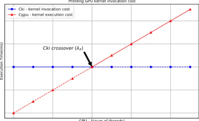
GPU - λ(num of threads)

Execution Time(ms)

Cki crossover (λX)

Profiling GPU kernel invocation cost Cki - kernel invocation cost

Cgpu - kernel execution cost

Figure 4.ALPyNA profiles a very simple kernel to discover

the minimum work rate required to keep the GPU busy sequentially within the generated GPU kernel. The loop in

Dseq(s)={Fk}is executed sequentially by the interpreter

calling GPU kernels executing the computation represented

by loopsDgpu(s)={Fi,Fj}andDgpu(s)={∅}.

To model the parallel execution cost of a statements

on a GPU, we measure the number of executions as the

product of the loop limits for the enclosingfor loops, as

before. However unlike the interpreter and CPU models, we now have a factor term to represent parallel execution, and hence reduce predicted execution time. The function

{G(L(f)), f ∈ D_gpu(s)}calculates the grid size and maps a

loop domain to a GPU hardware axis.Gmaximises

threads-per-block to calculate the number of grids within a thread-hierarchy.

While the number of threads allocated to execute on an SM can be greater than the number of CUDA cores in the SM, the maximum number of threads executing in parallel at any one time in an SM is the product of the number of warp

schedulers per SM (denotedv) and the warp size (denotedw).

The block structure of parallelized GPU code means we need to take into account precisely how the execution is mapped

onto SMs in a GPU (denotedu). For a statements, we denote

the amount of work done in each GPU kernel invocation as

λexec(s)(Equation6). Intuitively, if the GPU had an infinite

number of SMs, then termд.v.w would provide the parallel

speed-up. The ACM also calculates the cost of serializing execution of thread blocks in excess of the actual number of SMs. λexec(s)=lд u m × 1 д.v.w × Ö f∈ D_gpu(s) L(f) × Ö f∈ D_gpu(s) L(f) д= Ö f∈ Dgpu(s) G(L(f)) (6)

Modelling GPU Starvation.ALPyNA maintains

loop-carried dependences on code transformed for the GPU by scheduling the outermost loop iterations to execute in the

CPython interpreter. The GPU executes JIT compiled binary code much faster than the interpreter. If the interpreter exe-cutes each kernel invocation faster than the GPU can execute the kernel, each kernel is queued for execution on the GPU and overall execution time is bound by kernel execution. Otherwise, the GPU will finish each kernel before the

inter-preter can schedule the next one, and the GPU isstarvedof

work.

There are two cases to consider as shown in Equation7.

If all the loops around a statements are parallelizable, i.e.

Dseq(s)=∅, the code is transformed into a single invocation

of a kernel that executes all loop iterations ofD(s)on the

GPU. Hence there is a single kernel invocation latency cost

Ckivm. OtherwiseDseq(s) , ∅ and the execution cost is

the greater of the kernel invocation or the GPU execution

cost. HereIgpu(s)is the cost of executing a single instance

of the compiled kernel that represents statements. This

scenario arises in the running example (Listing3) where

Dseq(s)={F_k}.

Cgpu(s)=max Ckivm,λexec(s).Igpu(s) Ö

f∈ D_seq(s)

L(f)

ifDseq(s),∅

Cgpu(s)=Ckivm+λexec(s).Igpu(s)

ifDseq(s)=∅

(7)

Figure4depicts how for smaller amounts of parallel work,

the GPU kernel completes early and the interpreter loop execution time dominates. However once there is enough work in each kernel invocation to keep the GPU busy, GPU execution time dominates. This threshold varies depending on the relative performance of the GPU and the interpreter. To ascertain the GPU invocation cost threshold for each hardware setup, a very simple statement is profiled once at installation time. We use a two dimensional loop where only the inner loop can be parallelized. We profile this loop nest in ALPyNA using varying domain sizes to arrive at the GPU throttling threshold. The profiling starts at a parallel

domain size{L(f)=w|f ∈ Dpar(s)}and the domain size is

increased exponentially until the profiler detects execution time has gone beyond its inflexion point. The profiler then interpolates the number of threads at the inflection point

and calculatesλexec (Equation7) for the domain size at the

inflection point.

We seek to estimate the amount of GPU parallel work (in terms of domain sizes) required to overcome the kernel

invocation costCkivm, and designate this valueλX. At the

kernel invocation cost threshold, we assume the relationship

Ckivm≡ λX ×Igpu(s)

(8)

Profiling the simplest statementsto determine the

cross-over pointλX, provides a maximal number of threads beyond

which GPU execution time will dominate for any statements.

For a kernel representing more complex statements, this as-sumption leads to the ACM selecting a higher, (conservative), threshold of parallel work to offload to the GPU. Substituting

Ckivminto Equation7the estimated cost of executing each

kernel is shown in Equation9.

Cgpu(s)=max(λx,λexec(s)).Igpu(s). Ö f∈ D_seq(s)

L(f)

ifDseq(s)_,∅

Cgpu(s)=(λx+λexec(s)).Igpu(s)

ifDseq(s)=∅

(9)

The full cost of executing the loop nest with outermost

forloop f on the GPU is the summation in Equation10

whereCxfer(GPU)is the data transfer cost outlined next.

Tgpu(f)=Cxfer(f)+ Õ s∈ D(f)

Cgpu(s)

(10)

Modelling GPU transfer time.Executing on

accelera-tors like GPUs incurs overhead for transferring data between

the host CPU and the accelerator. We will see in Section5

that loop nests with light computational work are especially sensitive to the overheads of data transfer.

Following common practice we normalize data transfer time against the estimated cost of executing a very simple

statement in the CPython interpreter,Iint(s). Bandwidth

pro-filing of the PCIe bus on which the GPU resides is performed once at install time, along with the measurements of GPU

starvation factorλX (Section3.3, Equation8) and the CPU

JIT speed-up factorµ(Section3.4, Equation11).

While the transfer model is fairly standard, a novel fea-ture is that it is staged. That is ALPyNA identifies the set of vectors to be transferred to/from the GPU, and resolves their types and sizes at runtime. These are combined with the ahead-of-time bandwidth measurements to estimate the

transfer overhead,Cxfer(GPU).

3.4 Calibrating ACM

Like many cost models ACM takes parameters that charac-terise the specific execution platform, e.g. CPython and the Numba JIT compiler on a specific CPU, and CUDA on a

spe-cific GPU. Spespe-cifically the key cost equations,2,4and7take

parameters representing the predicted runtimeIplatform(s)of

executing a statementson a given platform, e.g.Icpu(s)in

Equation4. The platform costs for a statementsare

com-putedrelativeto the predicted interpreter costIint(s).

Calibration is required to determine the value of the model parameters for each execution platform, and this is achieved as follows.

The cost of executing a JIT compiled statement relative to the interpretation cost is profiled once at install time. A

(Section3.3) is used to relate the runtimes of JIT compiled, and CPython interpreted code. The array size in the loop nest is chosen to ensure that there is only one cache miss (on the first iteration). The relative performance factor obtained is

designated asµin Equation11. This provides a close

approx-imation of the relative runtimes of compiled and interpreted code without caching, and allows us to separately account for caches when comparing CPU and GPU runtimes.

µ=_IIint(s)

cpu(s) (11)

The relative cost of GPU execution clearly depends on the

relative clock frequencies of the CPU and GPU,fcpuandfдpu.

Moreover, Armih et al [4] and Belikov et al [6] both report

the size of the last level cache as a significant factor while comparing relative performance of data intensive programs on heterogeneous platforms. The last level cache (L2) on

the GPULCgpuis shared by all Symmetric Multiprocessors

(SMs). Each SM has its own set of L1 caches. For example in the NVIDIA Pascal (GP104) each SM has two L1 caches

[33]. This cache sharing is represented by the factorσ =

num_SM×L1_caches_per_SMin Equation12that computes relative GPU/CPU performance. There is no cache sharing factor for the CPU as Numba JIT compiles code for a single core and we assume that this core has exclusive use of the

L3 cache (LCcpu).

Icpu(s) Igpu(s) =ψ≈

fдpu× LCgpu/σ

fcpu×LCcpu (12)

Equation13shows how the cost of GPU execution relative

to the interpreter is directly computed as the product of

CPU/GPU cost and the interpreter/CPU ratioµ(Equation11).

Iint(s)

Igpu(s)≈µ×ψ (13)

Substituting Equations11,12and13into Equations2,4

and7allows ALPyNA to compare the predicted runtimes

on each execution platform and select the platform with

minimum cost,i.e.min(Tint,Tcpu,Tgpu).

3.5 ALPyNA Implementation

ACM is integrated into ALPyNA by annotating each state-ment in the lightweight ‘loop landmarks’ data structure

(Sec-tion2.2) with its relative cost when loop nest dependence

analysis takes place at runtime. ALPyNA’s runtime analysis and introspection capabilities enable aggressive discovery of opportunities to parallelize and estimate costs. This ap-proach minimises overheads as the cost model is constructed while resolving runtime dependences.

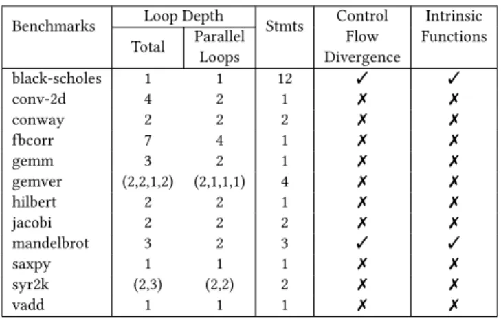
Table 1.Benchmark characteristics described as the set of

loops surrounding each statement, e.g. syr2k has two loops around the first statement and three around the second. Only some loops are parallelized.

Benchmarks Loop Depth Stmts Control Flow Divergence Intrinsic Functions Total Parallel Loops black-scholes 1 1 12 ✓ ✓ conv-2d 4 2 1 ✗ ✗ conway 2 2 2 ✗ ✗ fbcorr 7 4 1 ✗ ✗ gemm 3 2 1 ✗ ✗ gemver (2,2,1,2) (2,1,1,1) 4 ✗ ✗ hilbert 2 2 1 ✗ ✗ jacobi 2 2 2 ✗ ✗ mandelbrot 3 2 3 ✓ ✓ saxpy 1 1 1 ✗ ✗ syr2k (2,3) (2,2) 2 ✗ ✗ vadd 1 1 1 ✗ ✗

4

Experimental Setup

ACM is evaluated using 12 loop-intensive benchmarks from

the BLAS routines in the Polybench suite [29], the Numba

benchmarks, and from domains like finance (black-scholes) and digital signal processing (fbcorr).

The benchmarks represent a variety of characteristics that test ACM’s prediction capabilities for a variety of moderately

complex loop nests as summarised in Table1. Benchmarks

likesaxpyandvaddare extremely simple: a single loop with

just a single statement, and are embarrassingly parallel.

Con-trol flow divergence is encountered inblack-scholesand

man-delbrot. These loop nests also have pure (math) function calls that are mapped onto CUDA intrinsics in GPU kernels.

Ma-trix multiplication (gemm) andconv-2dare perfect loop nests

(every statement is dominated by every loop in the loop nest) but must execute some loops sequentially to maintain

depen-dence ordering. Imperfect loop nests occur ingemverand

syr2k

4.2 Hardware Platforms

The evaluation is conducted on a server grade machine (M1)

and typical desktops (M2,M3).M1has a Xeon E5-2620v4

octa core CPU with a 20MB L3 cache and a clock frequency of 2.1GHz that can be ‘Turboboost’ed to 3GHz. It has 16GB

(2×8GB) DDR4 RAM with a memory bus speed of 2133MHz.

M2has a Core i7-6700 quad core CPU with an 8MB L3

cache clock and a clock frequency of 3.4GHz, that can be

boosted to 3.9GHz. It has 16GB DDR4 (2×8GB) RAM with a

memory bus speed of 2133MHz. In a third machine

configu-ration (M3) the CPU frequency of machineM2is limited to

800MHz leaving all other parameters the same.

M1’s GPU is an NVIDIA Titan-XP (GP102) with a clock frequency of 1.4GHz and 12GB of GDDR5 RAM. It has 30

32K 64K 128K 256K 512K 1M 2M 4M 8M 16M 0 1 2 3 4 5 mispredict penalty cpu cpu cpu cpu

gpu gpu gpu gpu gpu gpu black-scholes 16 x 1632 x 3264 x 64_{128 x 128256 x 256512 x 512}1K x 1K2K x 2K4K x 4K8K x 8K_{16K x 16K} 0 1 2 3 4 5 mispredict penalty

cpu cpu cpu cpu gpu

gpu gpu gpu gpu gpu gpu convolution-2d 16 x 16 32 x 32 _{64 x 64 128 x 128 256 x 256 512 x 512 1K x 1K} 0 1 2 3 4 5 mispredict penalty

cpu cpu cpu cpu cpu cpu gpu

conway 16x8x256x25616x16x256x25616x8x512x51216x16x512x51216x8x1Kx1K16x16x1Kx1K 0 1 2 3 4 5 mispredict penalty

gpu gpu gpu gpu gpu gpu

fbcorr 16 x 16 32 x 32 64 x 64 128 x 128256 x 256512 x 512 1K x 1K 2K x 2K 0 1 2 3 4 5 mispredict penalty

cpu cpu cpu cpu

gpu

gpu gpu gpu

gemm 8 x 8 16 x 1632 x 3264 x 64_{128 x 128256 x 256512 x 512}1K x 1K2K x 2K4K x 4K8K x 8K_{16K x 16K} 0 1 2 3 4 5 mispredict penalty

cpu cpu cpu cpu cpu cpu cpu cpu cpu cpu cpu cpu gemver 16 x 16 32 x 32 64 x 64128 x 128256 x 256512 x 5121K x 1K 2K x 2K 4K x 4K 0 1 2 3 4 5 mispredict penalty

cpu cpu cpu cpu cpu cpu gpu gpu gpu

hilbert 4 x 4 _{8 x 8 16 x 1632 x 3264 x 64} 128 x 128256 x 256512 x 5121K x 1K2K x 2K 0 1 2 3 4 5 mispredict penalty

cpu cpu cpu cpu cpu cpu cpu cpu

gpu gpu jacobi 8 x 8 _{16 x 16 32 x 32 64 x 64 128 x 128256 x 256512 x 512 1K x 1K} 0 1 2 3 4 5 mispredict penalty

cpu cpu cpu cpu cpu gpu gpu gpu

mandelbrot 1K 2K 4K 8K 16K 32K 64K 128K256K512K 1M 2M 4M 8M 16M 32M 0 2 4 6 8 10

mispredict penalty cpu cpu cpu cpu cpu cpu cpu cpu cpu gpu

gpu

gpu gpu gpu_{gpu gpu} saxpy 8 x 8 16 x 1632 x 3264 x 64128 x 128256 x 256512 x 5121K x 1K2K x 2K4K x 4K 0 1 2 3 4 5 mispredict penalty

cpu cpu cpu cpu cpu gpu gpu gpu gpu gpu

syr2k 1K 2K 4K _{8K 16K 32K 64K 128K256K512K 1M 2M 4M 8M 16M} 0 2 4 6 8 10

mispredict penalty cpu cpu cpu cpu cpu cpu cpu cpu cpu gpu

gpu

gpu gpu gpu gpu vadd

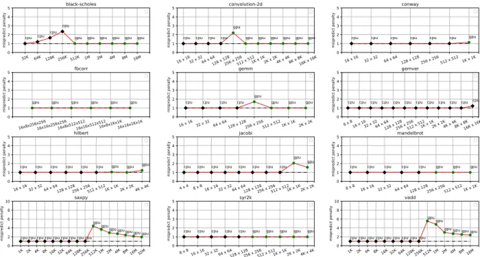
Figure 5.ALPyNA Cost Model misprediction penalties for 12 loop-intensive benchmarks with varying domain sizes on

platformT1. Misprediction slowdown is the ratio of predicted device runtime and faster device runtime, so optimal is 1.0.

SMs and a 3MB last level cache (L2).M2/M3have an NVIDIA

GeForce GTX-1060 with a clock frequency of 1.5GHz and 3GB of GDDR5 RAM. It has 9 SMs and a 1.5MB L2 cache. In both GPUs each SM has 128 CUDA cores, 4 warp schedulers

and two L1 caches [33]. Data transfer uses a PCI-Express

(PCIe 3.0) bus with the GPU as the only peripheral, and it negotiates to use 16 channels (x16).

The experiments are conducted on similar software stacks

as follows (M1,M2/M3). A native x86–64 Linux kernel (v4.15,

v4.9); CPython interpreter (v3.6.9, v3.5.3); PyPy (v7.3.1); Numpy (v1.13.3, v1.13.3); Numba (v0.34, v0.33); and CUDA (v8.0.61, v8.0.44). We identify the combined hardware and software

stacks as target platformsT1,T2andT3.

4.3 ACM Usage

Before using ACM on a target CPU/GPU platform the values

ofλX,µ(Eqs.11and8) and relative GPU bandwidth (Section

3.3) must be profiled. A 10% safety margin is used over the

predicted inflection point where the interpreter is able to

keep the GPU busy. The calculation of BW_I

gpu, i.e. data transfer

speeds in execution time units(Iint), is done while profiling

for the valueµto ensure consistency.

The Numba compiler compiles and executes single threaded code. During experimentation no other cores execute com-putationally intensive code and hence the core can reach maximum frequencies without being throttled.

The selection of CPU or GPU to target for JIT compilation is dependent on the overall computation size, proportion of parallel computation, and data movement costs. The ef-fectiveness of ACM’s device selection for JIT compilation is measured across a wide range of iteration domain sizes. Iteration domain sizes are increased by doubling the loop domain size of each loop within the benchmarks. Reported runtimes are the arithmetic mean of 5 executions.

4.4 Comparative Baselines

For each domain size, execution time on the ACM predicted device is compared with two baselines: (1) execution time on the optimal device identified by an ‘oracle’ predictor; (2) execution time on the device selected by a two-class support vector machine (SVM), i.e. a representative supervised learn-ing model. The SVM is trained on the 12 benchmarks uslearn-ing per-benchmark leave-one-out cross-validation. We train sep-arately for each of the three evaluation platforms. We use the oracle predictor value to label training set instances. The feature vector comprises static code structure metrics (cf.

Table1), input size and dimensions, and raw execution times

on both target devices. All feature values are scaled with

min-max normalization to the range[0,1].

PyPy [3] is a tracing JIT compiler to speed-up Python

execution. Execution time of CPU and GPU code generated

by ALPyNA for the 12 benchmarks (Section4.1) is compared

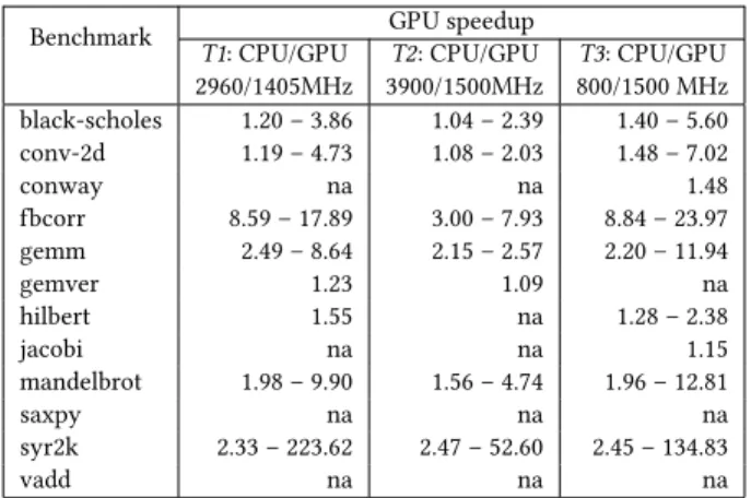
Table 2.Range of ALPyNA GPU speedups across iteration domain sizes. Some benchmarks have no speedup.

Benchmark GPU speedup

T1: CPU/GPU 2960/1405MHz T2: CPU/GPU 3900/1500MHz T3: CPU/GPU 800/1500 MHz black-scholes 1.20 – 3.86 1.04 – 2.39 1.40 – 5.60 conv-2d 1.19 – 4.73 1.08 – 2.03 1.48 – 7.02 conway na na 1.48 fbcorr 8.59 – 17.89 3.00 – 7.93 8.84 – 23.97 gemm 2.49 – 8.64 2.15 – 2.57 2.20 – 11.94 gemver 1.23 1.09 na hilbert 1.55 na 1.28 – 2.38 jacobi na na 1.15 mandelbrot 1.98 – 9.90 1.56 – 4.74 1.96 – 12.81 saxpy na na na syr2k 2.33 – 223.62 2.47 – 52.60 2.45 – 134.83 vadd na na na

enabled. For each benchmark, PyPy is allowed to warm up to enable tracing and JIT compilation before timing mea-surements are taken. A timeout of five hours is used for benchmark execution with PyPy.

5

Evaluation

GPU Speedups.Table2shows the range of speedups

ob-tained using the GPU for the benchmarks on each machine. It shows that most benchmarks benefit from exploiting the GPU at some iteration domain sizes; even those that show no benefit can be useful ACM test cases as outlined below.

ACM Misprediction Penaltyis reported in Figure5for

each of the 12 benchmarks on target platformT1. At each

do-main size it shows the platform device (CPU or GPU) selected

by the cost model, along with anymisprediction penalty. The

misprediction penalty is the ratio between runtime on the selected device and runtime on the optimal device, so 1.0 is optimal. Note the logarithmic x-axis for relevant domain sizes. ACM delivers similar misprediction penalties for the

benchmarks onT2andT3, and corresponding

mispredic-tion penalty graphs are available in supplementary online

materials [16].

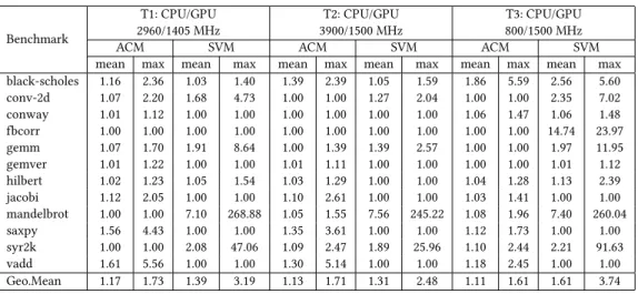
For all benchmarks and platforms Table3shows the

geo-metric mean penalties over all domain sizes and the maxi-mum penalties. ACM provides entirely accurate predictions

for four benchmarks onT2andT3and for three onT1. The

mean penalties for different benchmarks vary from 1.0

(op-timal) to 1.61, 1.39, and 1.86 forT1,T2, andT3respectively.

The last row of Table3shows the mean penalty and mean

per-benchmark maximum penalty on each platform. The geometric mean penalty across all our experiments is 1.136. We observe the SVM mean penalty is worse than ACM on each platform. Significant worst-case outliers for SVM maxi-mum penalties contribute to high SVM mean per-benchmark maximum penalty on each platform. This may indicate limi-tations in the training set used for SVM classification.

Misprediction Intervals.Figure6shows CPU and GPU

benchmark runtimes onT1with ACM and SVM

mispredic-tion intervals highlighted. Between measured domain sizes the misprediction is interpolated. ACM delivers similar

mis-prediction intervals for the benchmarks onT2andT3[16].

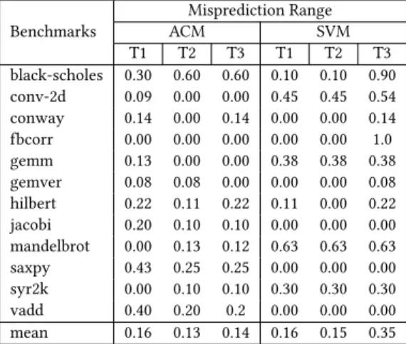
Table4shows the relative proportion of each input domain

that is mispredicted. The mean misprediction proportion across all benchmarks is 0.143. ACM has the same or smaller misprediction intervals than the SVM predictor for 5, 6 and

9 of the 12 benchmarks onT1,T2andT3respectively.

The ACM misprediction intervals are generally small for benchmarks with sharply diverging CPU and GPU runtime

curves likeconv-2d,gemm,mandelbrotandsyr2k. The

excep-tions areblack-scholesonT2andT3, where ACM mispredicts

that the CPU execution will be faster over the initial range before correctly selecting the GPU at medium to large do-main sizes. For the benchmarks that have no dodo-main sizes where the GPU is faster, ACM correctly predicts this at all

domain sizes forgemverandconway, but mispredicts at large

domain sizes forsaxpyandvadd.

Comparison with PyPy.Figure6also compares PyPy

execution time with ALPyNA CPU and GPU execution times

for each benchmark on platformT1. Both CPU and GPU

code generated by ALPyNA is faster than PyPy across all

domain sizes for 10 benchmarks onT1andT3, and for 9

benchmarks onT2. Forjacobi, PyPy is slower than ALPyNA

CPU execution across all domain sizes onT1,T2andT3.

ForjacobiPyPy is slower than ALPyNA CPU execution at

all domain sizes onT1,T2andT3. It is faster than ALPyNA

GPU but slower than ALPyNA CPU at the two smallest

iter-ation domain sizes. Forsyr2kPyPy is slower than ALPyNA’s

CPU code and faster than ALPyNA’s GPU code at the small-est four iteration domain sizes on all three platforms. The sit-uation reverses at larger domain sizes where PyPy is slower than ALPyNA’s GPU code but faster than ALPyNA’s CPU

code. For bothjacobiandsyr2k, utilising the device chosen

by ACM at each domain size is faster than PyPy.

Loop Nest Characteristics.The benchmarks represent

a range of different loop nests, and we investigate the impact of these on the cost model.

Inembarrassingly parallelloop nests, every loop

domi-nating a statement can safely be executed in parallel:

black-scholes,conway,hilbert jacobi,saxpyandvaddare in this

class. For some of these applications, the data transfer over-head is so large, relative to the actual computation, that GPU execution never outperforms CPU execution. This is partic-ularly noticeable for single loops with tiny loop bodies that

iterate linearly over input arrays. Referring back to Table1,

we observe thathilbert,jacobi,saxpyandvaddfall into this

category. This is reflected in these benchmarks’ performance on all three platforms, where CPU execution is optimal across

all domain sizes. For instance, Figure6shows that parallel

GPU execution cannot match sequential CPU execution for these simple embarrassingly parallel benchmarks, since data

32K 64K 128K 256K 512K 1M 2M 4M 8M 16M

10−3 10−1 101 103

Exec Time (sec)

black-scholes cpu-perf gpu-perf pypy-perf 16 x 1632 x 3264 x 64_{128 x 128256 x 256512 x 512}1K x 1K2K x 2K4K x 4K8K x 8K_{16K x 16K} 10−5 10−2 101 104

Exec Time (sec)

convolution-2d cpu-perf gpu-perf pypy-perf 16 x 16 32 x 32 64 x 64 _{128 x 128 256 x 256 512 x 512} 1K x 1K 10−5 10−2 101

Exec Time (sec)

conway cpu-perf gpu-perf pypy-perf 16x8x256x25616x16x256x25616x8x512x51216x16x512x51216x8x1Kx1K16x16x1Kx1K 10−1 101 103 105

Exec Time (sec)

fbcorr cpu-perf gpu-perf pypy-perf 16 x 16 32 x 32 _{64 x 64 128 x 128256 x 256512 x 512 1K x 1K 2K x 2K} 10−4 10−1 102

Exec Time (sec)

gemm cpu-perf gpu-perf pypy-perf 8 x 8 16 x 1632 x 3264 x 64_{128 x 128256 x 256512 x 512}1K x 1K2K x 2K4K x 4K8K x 8K_{16K x 16K} 10−5 10−2 101 104

Exec Time (sec)

gemver cpu-perf gpu-perf pypy-perf 16 x 16 32 x 32 64 x 64128 x 128256 x 256512 x 5121K x 1K 2K x 2K 4K x 4K 10−5 10−2 101

Exec Time (sec)

hilbert cpu-perf gpu-perf pypy-perf 4 x 4 _{8 x 8 16 x 1632 x 3264 x 64} 128 x 128256 x 256512 x 5121K x 1K2K x 2K 10−5 10−2 101

Exec Time (sec)

jacobi cpu-perf gpu-perf pypy-perf 8 x 8 16 x 16 32 x 32 _{64 x 64 128 x 128256 x 256512 x 512 1K x 1K} 10−3 100 103

Exec Time (sec)

mandelbrot cpu-perf gpu-perf pypy-perf 1K 2K 4K 8K 16K 32K 64K 128K256K512K 1M 2M 4M 8M 16M 32M 10−5 10−2 101

Exec Time (sec)

saxpy cpu-perf gpu-perf pypy-perf 8 x 8 16 x 1632 x 3264 x 64128 x 128256 x 256512 x 5121K x 1K2K x 2K4K x 4K 10−5 10−2 101 104

Exec Time (sec)

syr2k cpu-perf gpu-perf pypy-perf 1K 2K 4K _{8K 16K 32K 64K 128K 256K 512K 1M 2M 4M 8M 16M} 10−5 10−2 101

Exec Time (sec)

vadd cpu-perf

gpu-perf pypy-perf

Figure 6.Misprediction intervals of ALPyNA Cost Model (shaded blue), an SVM predictor (shaded red), and both (shaded

purple) for 12 loop-intensive benchmarks with varying domain sizes on platformT1. ACM’s domain crossover point is

interpolated from the measured values. Execution time of ALPyNA’s CPU and GPU code is also compared with PyPy execution. Execution time (y–axis) is plotted on a logarithmic scale.

Table 3.ACM misprediction penalties for all benchmarks on all platforms: Geometric Mean Penalties across all input sizes,

and Maximum Penalties.

Benchmark T1: CPU/GPU 2960/1405 MHz T2: CPU/GPU 3900/1500 MHz T3: CPU/GPU 800/1500 MHz

ACM SVM ACM SVM ACM SVM

mean max mean max mean max mean max mean max mean max black-scholes 1.16 2.36 1.03 1.40 1.39 2.39 1.05 1.59 1.86 5.59 2.56 5.60 conv-2d 1.07 2.20 1.68 4.73 1.00 1.00 1.27 2.04 1.00 1.00 2.35 7.02 conway 1.01 1.12 1.00 1.00 1.00 1.00 1.00 1.00 1.06 1.47 1.06 1.48 fbcorr 1.00 1.00 1.00 1.00 1.00 1.00 1.00 1.00 1.00 1.00 14.74 23.97 gemm 1.07 1.70 1.91 8.64 1.00 1.39 1.39 2.57 1.00 1.00 1.97 11.95 gemver 1.01 1.22 1.00 1.00 1.01 1.11 1.00 1.00 1.00 1.00 1.01 1.12 hilbert 1.02 1.23 1.05 1.54 1.03 1.29 1.00 1.00 1.04 1.28 1.13 2.39 jacobi 1.12 2.05 1.00 1.00 1.10 2.61 1.00 1.00 1.03 1.41 1.00 1.00 mandelbrot 1.00 1.00 7.10 268.88 1.05 1.55 7.56 245.22 1.08 1.96 7.40 260.04 saxpy 1.56 4.43 1.00 1.00 1.35 3.61 1.00 1.00 1.12 1.73 1.00 1.00 syr2k 1.00 1.00 2.08 47.06 1.09 2.47 1.89 25.96 1.10 2.44 2.21 91.63 vadd 1.61 5.56 1.00 1.00 1.30 5.14 1.00 1.00 1.18 2.45 1.00 1.00 Geo.Mean 1.17 1.73 1.39 3.19 1.13 1.71 1.31 2.48 1.11 1.61 1.61 3.74

transfer overhead is included in total execution time. This in-terplay between data transfer overhead and GPU parallelism has motivated the design of ACM; similar ideas are seen in

other cost models as outlined in Section6.

Partially parallelizableloops have loop-carried dependences

that constrain some loops to be executed sequentially in the

CPython interpreter:con-2d,fbcorr,gemm,gemver,

mandel-brotandsyr2kare in this class. For such loops the amount

of parallelism obtained is dependent on the domain sizes of the parallelizable loops and the amount of work scheduled on the GPU.

Table 4.Ratio of mispredicted/correct ranges for all

bench-marks on platformsT1,T2andT3using ACM and an SVM

predictor Benchmarks Misprediction Range ACM SVM T1 T2 T3 T1 T2 T3 black-scholes 0.30 0.60 0.60 0.10 0.10 0.90 conv-2d 0.09 0.00 0.00 0.45 0.45 0.54 conway 0.14 0.00 0.14 0.00 0.00 0.14 fbcorr 0.00 0.00 0.00 0.00 0.00 1.0 gemm 0.13 0.00 0.00 0.38 0.38 0.38 gemver 0.08 0.08 0.00 0.00 0.00 0.08 hilbert 0.22 0.11 0.22 0.11 0.00 0.22 jacobi 0.20 0.10 0.10 0.00 0.00 0.00 mandelbrot 0.00 0.13 0.12 0.63 0.63 0.63 saxpy 0.43 0.25 0.25 0.00 0.00 0.00 syr2k 0.00 0.10 0.10 0.30 0.30 0.30 vadd 0.40 0.20 0.2 0.00 0.00 0.00 mean 0.16 0.13 0.14 0.16 0.15 0.35

There is no clear difference between the ACM mispredic-tion penalties and mispredicmispredic-tion intervals for embarrassingly and partially parallelizable loops.

6

Related Work

Execution time prediction has a very long history. Worst case execution time (WCET) analysis aims to precisely and

conservatively predictabsoluteruntime by static analysis or

dynamic profiling [37]. To be lightweight ACM uses static

analysis as far as possible. However rather than predicting

absoluteruntimes it compares therelativeruntimes on a set

of heterogeneous compute platforms.

Cost models, or resource analyses, are commonly used to predict runtimes in parallel systems, e.g. to inform task

scheduling. Trinderet alpresent a wide-ranging survey [34],

and using their classification ACM is an abstract relative parallel cost model, based on heuristic linear equations, and parameterized by a parallel implementation model of the underlying hardware.

Static Languages.Loop nests have been widely and

suc-cessfully automatically parallelized in compiled languages,

e.g. [7]. Many auto-parallelizing compilers use a cost model

to determine what to parallelize. Compared with a dynamic language like Python, compilers for static languages have far more information about the loop nests.

A rapidly growing body of work studies GPU performance

prediction. For example [22] models standard GPU

architec-tures and, like ACM, derives parameterized mathematical equations to estimate GPU kernel runtimes. There are a va-riety of more sophisticated GPU performance prediction

techniques making use of analytical models like [5,32].

Other approaches rely on the program being written as

al-gorithmic skeletons, e.g. the Grophecy tool [28] predicts GPU

runtime based on CPU runtime. Other predictions of GPU runtime based on CPU profiling rely on machine learning,

e.g. [2] that builds a regression model for cross-architecture

performance prediction.

Using machine learning rather than derived analytical models for GPU runtime prediction has become increasingly

common, e.g. [39]. However an empirical comparison with

analytical cost models shows that the analytical models

pro-vide greater accuracy [1]. Analytic models are parameterised

with hardware and program values, and ACM’s dynamic analytic system determines some of these at runtime.

Currently there is intense interest in automatically exe-cuting OpenMP loop nests on heterogeneous architectures. Here, as in other auto-parallelization the importance of aug-menting static analysis with runtime values is recognised,

e.g. [9]. This approach compiles parallel CPU and GPU code

for the loop nest and uses a staged cost model to select what code to run. ACM is similarly staged, but ALPyNA uses JIT compilation to dynamically create custom GPU kernels that are tailored to the exact dependences that arise in each in-stance of the loop nest. ACM also reflects the idea that the execution schedule of the loops may change along with the structure of the kernels.

Speculative parallelization of tightly nested loops in man-aged language runtimes is an attractive approach to obtain

speed ups [30,31,36]. Leung et al [25] attempt to cost

po-tential execution on a GPU compared to a CPU. Extensive profiling of absolute time required for execution of a Java bytecode on CPU and GPU is used to arrive at an estimate for GPU execution time. ACM uses a predictor parameterised on the hardware characteristics of each device such as fre-quency, cache sharing and also model runtime bottlenecks such as starvation effects.

Some systems that target heterogeneous platforms exploit sophisticated managed language runtimes. For example

Tor-nadoVM operates on annotated loop-intensive Java [10]. It

uses task graphs to express dependencies and selects be-tween CPU, GPU and FPGA targets. It exhaustively samples loop execution profiles for all available targets and selects the best target for future scheduling. ACM and ALPyNA also exploit Python’s sophisticated managed runtime, but (1) use an analytical model where TornadoVM uses profiling and (2) avoid eagerly generating code for all targets. That is, code is only JIT compiled if ACM identifies the target as the best.

Some recentDynamic Languagecompilers dynamically

generate code for heterogeneous compute devices. There are various approaches to automatically select the most ap-propriate compute device at runtime for particular program

fragments like methods or loop nests. Hayashi et al [13] and

Kim et al [19] study CPU and GPU execution of Java code and

advocate machine learning for selecting the target platform for parallel stream API calls. Extracted features for input to the trained machine learning model include the parallel loop range, which must be acquired by runtime introspection as in ACM.

Other researchers have recognized the importance of Python for end user programming in scientific domains. For example the Selective Embedded Just-in-Time Specialization (SEJITS)

project [17] enables expert users to embed domain-specific

optimizations for key computational kernels such as ma-trix algebra. These optimizations are dynamically invoked and high-performance (typically native C) code is generated for the compute-intensive portions of the code. In contrast ALPyNA does not require expert ‘intervention’ to generate kernels and dynamically selects the execution platform.

7

Conclusions

This paper presents the design, implementation and evalu-ation of ACM, the first analytical cost model that supports the automatic runtime exploitation of GPUs in a dynamic language. The model is staged and lightweight, and is used to select between compute devices to effectively parallelize moderately complex Python loop nests on commodity het-erogeneous platforms using the ALPyNA framework.

For each instance of a loop nest, ACM dynamically predicts the relative runtimes on alternative devices so that ALPyNA can select the fastest. The models for the CPython interpreter, and for JIT compiled CPU execution are relatively standard, but the GPU model is both novel and elaborate. It accounts for key costs like data transfer time, and for starvation ef-fects etc. All of the platform models are parametric in key characteristics of the platforms, like cache size and sharing,

and warp size on the GPU (Section3).

We report a systematic evaluation of ACM on three hetero-geneous platforms using 12 standard loop-intensive Python benchmarks, and covering a wide range of domain sizes

(Sec-tion4). The cost model proves to be effective, with small

misprediction ranges (Table3) and a mean misprediction

penalty of just 13.6% slowdown, relative to optimal, across

all benchmarks (Section5). The cost model also outperforms

a trained SVM.

Future WorkAn immediate avenue for future work is to

evaluate the cost model on additional heterogeneous systems. Currently ACM does not account for the overhead of runtime compilation. Hence interpretive execution is never selected over JIT compilation even when it would reduce runtime for small iteration domains. For frequently executed kernels it

helps that Numbapersistsgenerated code in a compilation

cache. We expect it will be relatively easy to extend ACM to account for runtime compilation overheads, e.g. using

models like [27].

ACM has been designed to be extensible and we envisage extending ACM as underlying technologies improve. An

ex-tension might model GPUkernel fusion[35] if ALPyNA adds

supports for this. A further extension might model vectorized execution on CPU or other parallel code generation.

Acknowledgments

The authors would like to thank Alexandre Bergel for his friendly and constructive shepherding of this paper. We also thank the anonymous reviewers for their helpful sugges-tions.

This material is based upon work supported by the UK Engineering and Physical Sciences Research Council under Grants EP/M508056/1 and EP/V000349/1.

References

[1] M. Amarís, R. Y. de Camargo, M. Dyab, A. Goldman, and D. Trystram. 2016. A comparison of GPU execution time prediction using machine learning and analytical modeling. InNCA. 326–333. https://doi.org/ 10.1109/NCA.2016.7778637

[2] N. Ardalani, C. Lestourgeon, K. Sankaralingam, and X. Zhu. 2015. Cross-Architecture Performance Prediction (XAPP) Using CPU Code to Predict GPU Performance. InProc. MICRO. https://doi.org/10.1145/ 2830772.2830780

[3] H. Ardö, C. F. Bolz, and M. Fijałkowski. 2012. Loop-Aware Optimiza-tions in PyPy’s Tracing JIT. InProc. DLS. https://doi.org/10.1145/ 2384577.2384586

[4] K. Armih, G. Michaelson, and P. Trinder. 2011. Cache Size in a Cost Model for Heterogeneous Skeletons. InProc. HLPP. https://doi.org/10. 1145/2034751.2034755

[5] S. Baghsorkhi, M. Delahaye, S. Patel, W. Gropp, and W. Hwu. 2010. An Adaptive Performance Modeling Tool for GPU Architectures. InProc. PPoPP. https://doi.org/10.1145/1693453.1693470

[6] E. Belikov, H.-W. Loidl, G. Michaelson, and P. Trinder. 2012. Architecture-aware cost modelling for parallel performance porta-bility. InSoftware Engineering 2012. Workshopband.

[7] Z. Bozkus, A. Choudhary, G. Fox, T. Haupt, S. Ranka, and M-Y Wu. 1994. Compiling Fortran 90D/HPF for distributed memory MIMD computers.J. Parallel and Distrib. Comput.(1994).

[8] B. Catanzaro, M. Garland, and K. Keutzer. 2011. Copperhead: Com-piling an Embedded Data Parallel Language. SIGPLAN Not.(2011).

https://doi.org/10.1145/2038037.1941562

[9] A. Chikin, J. N. Amaral, K. Ali, and E. Tiotto. 2019. Toward an Analyt-ical Performance Model to Select between GPU and CPU Execution. InProc. IPDPS. https://doi.org/10.1109/IPDPSW.2019.00068

[10] J. Fumero, M. Papadimitriou, F. Zakkak, M. Xekalaki, J. Clarkson, and C. Kotselidis. 2019. Dynamic Application Reconfiguration on Het-erogeneous Hardware. InProc. VEE. https://doi.org/10.1145/3313808. 3313819

[11] J. Fumero, M. Steuwer, L. Stadler, and C. Dubach. 2017. Just-In-Time GPU Compilation for Interpreted Languages with Partial Evaluation. InProc. VEE. https://doi.org/10.1145/3050748.3050761

[12] Design Guide. 2013. Cuda C programming guide.NVIDIA, July(2013).

https://docs.nvidia.com/cuda/archive

[13] A. Hayashi, K. Ishizaki, G. Koblents, and V. Sarkar. 2015. Machine-Learning-Based Performance Heuristics for Runtime CPU/GPU Selec-tion. InProc. PPPJ. https://doi.org/10.1145/2807426.2807429

[14] D. Jacob and J. Singer. 2019. ALPyNA: Acceleration of Loops in Python for Novel Architectures. InProc. ARRAY. https://doi.org/10.1145/ 3315454.3329956

[15] D. Jacob, P. Trinder, and J. Singer. 2019. Python Programmers Have GPUs Too: Automatic Python Loop Parallelization with Staged Depen-dence Analysis. InProc. DLS. https://doi.org/10.1145/3359619.3359743

[16] D. Jacob, P. Trinder, and J. Singer. 2020. Prediction Performance and Misprediction Interval Graphs of ALPyNA Cost Model for platforms

T2andT3. https://bitbucket.org/djichthys/alpyna/src/master/doc/ DLS20_graphs_T2_T3.pdf.

[17] S. Kamil, D. Coetzee, and A. Fox. 2011. Bringing parallel performance to Python with domain-specific selective embedded just-in-time spe-cialization. InConf. Python for Scientific Computing (SciPy). [18] K. Kennedy and J. R. Allen. 2001. Optimizing Compilers for Modern

Architectures: A Dependence-Based Approach. Morgan Kaufmann. [19] G. Kim, A. Hayashi, V. Sarkar, and G. Juckeland. 2018. Exploration of

Supervised Machine Learning Techniques for Runtime Selection of CPU vs. GPU Execution in Java Programs. InProc. WACCPD. [20] A. Klöckner. 2014. Loo.Py: Transformation-Based Code Generation

for GPUs and CPUs. InProc. ARRAY. https://doi.org/10.1145/2627373. 2627387

[21] A. Klöckner, N. Pinto, Y. Lee, B. Catanzaro, P. Ivanov, and A. Fasih. 2012. PyCUDA and PyOpenCL: A scripting-based approach to GPU run-time code generatio.Parallel Comput.(2012). https://doi.org/10. 1016/j.parco.2011.09.001

[22] K. Kothapalli, R. Mukherjee, M. S. Rehman, S. Patidar, P. J. Narayanan, and K. Srinathan. 2009. A performance prediction model for the CUDA GPGPU platform. InProc. HiPC. https://doi.org/10.1109/HIPC.2009. 5433179

[23] S. K. Lam, A. Pitrou, and S. Seibert. 2015. Numba: A LLVM-based Python JIT compiler. InProc. LLVM Compiler Infrastructure in HPC.

https://doi.org/10.1145/2833157.2833162

[24] T. Lengauer and R. Tarjan. 1979. A Fast Algorithm for Finding Dom-inators in a Flowgraph. ACM Trans. Program. Lang. Syst.(1979).

https://doi.org/10.1145/357062.357071

[25] A. Leung, O. Lhoták, and G. Lashari. 2009. Automatic Parallelization for Graphics Processing Units. InProc. PPPJ. https://doi.org/10.1145/ 1596655.1596670

[26] D. Luebke. 2008. CUDA: Scalable parallel programming for high-performance scientific computing. InProc. ISBI. https://doi.org/10. 1109/ISBI.2008.4541126

[27] G. Luo, T. Chen, and H. Yu. 2007. Toward a progress indicator for program compilation.Software: Practice and Experience(2007). https: //doi.org/10.1002/spe.792

[28] J. Meng, V. Morozov, K. Kumaran, V. Vishwanath, and T. Uram. 2011. GROPHECY: GPU Performance Projection from CPU Code Skeletons.

InProc. SC. https://doi.org/10.1145/2063384.2063402

[29] L.-N. Pouchet, U. Bondhugula, et al. 2020. The Polybench Benchmarks.

http://web.cse.ohio-state.edu/~pouchet.2/software/polybench. [30] M. Qunaibit, S. Brunthaler, Y. Na, S. Volckaert, and M. Franz. 2018.

Accelerating Dynamically-Typed Languages on Heterogeneous Plat-forms Using Guards Optimization. InProc. ECOOP. https://doi.org/10. 4230/LIPIcs.ECOOP.2018.16

[31] M. Samadi, A. Hormati, J. Lee, and S. Mahlke. 2012. Paragon: Collabo-rative Speculative Loop Execution on GPU and CPU. InProc. GPGPU.

https://doi.org/10.1145/2159430.2159438

[32] J. Sim, A. Dasgupta, H. Kim, and R. Vuduc. 2012. A Performance Anal-ysis Framework for Identifying Potential Benefits in GPGPU Applica-tions.SIGPLAN Not.(2012). https://doi.org/10.1145/2370036.2145819

[33] R. Smith. 2016. The NVIDIA GeForce GTX 1080 & GTX 1070 Founders Editions Review: Kicking Off the FinFET Genera-tion. https://www.anandtech.com/show/10325/the-nvidia-geforce-gtx-1080-and-1070-founders-edition-review/4.

[34] P. Trinder, M. Cole, K. Hammond, H.-W. Loidl, and G. J. Michaelson. 2013. Resource analyses for parallel and distributed coordination.

Concurrency and Computation: Practice and Experience(2013). [35] G. Wang, Y. Lin, and W. Yi. 2010. Kernel fusion: An effective method

for better power efficiency on multithreaded GPU. InProc. GreenCom-CPSCom. https://doi.org/10.1109/GreenCom-CPSCom.2010.102

[36] Z. Wang, D. Powell, B. Franke, and M. O’Boyle. 2014. Exploitation of GPUs for the Parallelisation of Probably Parallel Legacy Code. InProc. CC.

[37] R. Wilhelm, J. Engblom, A. Ermedahl, N. Holsti, S. Thesing, D. Whalley, G. Bernat, C. Ferdinand, R. Heckmann, T. Mitra, et al. 2008. The worst-case execution-time problem—overview of methods and survey of tools.ACM TECS(2008).

[38] M. Wolfe and U. Banerjee. 1987. Data dependence and its application to parallel processing. Proc. IJPP (1987). https://doi.org/10.1007/ BF01379099

[39] G. Wu, J. L. Greathouse, A. Lyashevsky, N. Jayasena, and D. Chiou. 2015. GPGPU performance and power estimation using machine learning. InHPCA. 564–576. https://doi.org/10.1109/HPCA.2015.7056063