Regularization of all-pole models for speaker verification under additive noise

PDF hosted at the Radboud Repository of the Radboud University

Nijmegen

The following full text is an author's version which may differ from the publisher's version.

For additional information about this publication click this link.

http://hdl.handle.net/2066/101969

Please be advised that this information was generated on 2017-12-06 and may be subject to

change.

Regularization of All-Pole Models for Speaker Verification

Under Additive Noise

Cemal Hanilc¸i

, Tomi Kinnunen

, Rahim Saeidi

, Jouni Pohjalainen

, Paavo Alku

, Figen Ertas¸

1

Department of Electronic Engineering, Uluda˘g University, Bursa, Turkey

School of Computing, University of Eastern Finland, Finland

Centre for Language and Speech Technology, Radboud University Nijmegen, Netherlands

Department of Signal Processing and Acoustics, Aalto University, Finland

Abstract

Regularization of linear prediction based mel-frequency cep-stral coefficient (MFCC) extraction in speaker verification is considered. Commonly, MFCCs are extracted from the discrete Fourier transform (DFT) spectrum of speech frames. In our re-cent study, it was shown that replacing the DFT spectrum esti-mation step with the conventional and temporally weighted lin-ear prediction (LP) and their regularized versions increases the recognition performance considerably. In this paper, we provide a through analysis on the regularization of conventional and temporally weighted LP methods. Experiments on the NIST 2002 corpus indicate that regularized all-pole methods yield large improvements on recognition accuracy under additive fac-tory and babble noise conditions in terms of both equal error rate (EER) and minimum detection cost function (MinDCF).

1. Introduction

Speaker verification aims to verify speaker’s identity from a given speech signal [1]. A speaker verification system con-sists of two modules: feature extraction (front-end) and pattern matching (back-end). In pattern matching, features extracted from a given speech input are compared to the claimed speaker’s model. Gaussian mixture models (GMMs) [2] and support vec-tor machines (SVMs) are two popular back-ends, while mel-frequency cepstral coefficients (MFCCs) are commonly used as acoustic features. MFCCs are generally obtained from the discrete Fourier transform (DFT),which is implemented with fast Fourier transform (FFT), spectrum of windowed speech frames.

Speaker verification accuracy under clinical and controlled conditions is high but decreases significantly under channel mismatch and in the presence of additive noise. Channel mis-match is the problem of having training and test speech samples from different types of channels or handsets, whereas additive noise refers to other interfering sound sources being added to the speech signal. In literature, several methods have been pro-posed to tackle channel mismatch and additive noise. These include, for instance, speech enhancement prior to feature ex-traction and feature normalization using cepstral mean and vari-ance normalization (CMVN). In addition, intersession compen-sation of speaker models [3] and score normalization [4] are commonly applied.

In [5], the present authors extracted MFCCs from para-metric all-pole spectral models based on linear prediction (LP)

[6] and its temporally weighted extensions [7]. This led to increased speaker verification accuracy over the standard FFT method under additive noise contamination. A possible expla-nation for this is that low-order all-pole models, due to smaller number of free parameters in comparison to FFT, exhibit less variations between clean and noisy utterances. Recently, in [8], the authors showed that using the regularized all-pole models to estimate magnitude spectrum in the feature extraction im-proves the speaker verification accuracy significantly. In the field of pattern recognition, regularization techniques are com-monly used for trading off between training and test errors to enhance classifier generalization [9] but they have been much less studied for feature extraction and speech parameterization [10]. In this paper, we would like to provide a through analysis of the regularized all-pole models for speaker verification under additive noise contamination.

Regularized LP (RLP) [10] is a parametric spectral model-ing method motivated from a speech codmodel-ing point of view for tackling a known problem in that field, over-sharpening of for-mants. RLP penalizes rapid changes in all-pole spectral en-velopes, thereby producing smooth spectra without affecting formant positions. However, RLP has not been applied to any recognition tasks to the best of our knowledge. Intuitively, the use of RLP is justified in speaker verification because it enables computing smooth spectral models and is therefore expected to reduce mismatch between training and test utterances. Since clean speech was used in [10], the present study will address the performance of RLP under additive noise contamination. Moreover, in [10] only boxcar (rectangular) window was used for autocorrelation domain windowing to compute the penalty function. Therefore, we study the effects of different autocor-relation windowing methods on recognition accuracy. Finally, in addition to conventional LP, we extend regularization to the temporally weighted variants of LP, weighted LP (WLP) [5] and stabilized weighted linear prediction (SWLP) [7].

2. Spectrum Estimation

2.1. Baseline FFT and LP Methods

MFCC features are generally obtained from the periodogram of a Hamming-windowed speech frame given by

SFFT(f) = N−1 X n=0 w(n)x(n)e−j2πnf /N 2 , (1)

wherefis the discrete frequency index,x= [x(0). . . x(N− 1)]T _{is a speech frame andw = [w(0) . . . w(N −1)]}T _is the Hamming window. The signalx(n)is assumed to be zero outside of the interval [0, N−1].

LP analysis [6] is based on the assumption that a speech sample,x(n), can be predicted as a weighted sum of itsp previ-ous samples,xˆ(n) =−Pp

k=1akx(n−k), wherex(n)is the

original speech sample,xˆ(n)is the predicted sample andpis the predictor order. Usually, the predictor coefficients{ak}pk=1

are obtained by minimizing the energy of the prediction resid-ual,e(n) =x(n)−xˆ(n) =x(n) +Pp

k=1akx(n−k). In the

autocorrelation method, the solution foralpopt= [a1, . . . , ap]T is given by

alpopt=−R− 1

lprlp, (2)

whereRlpis the Toeplitz autocorrelation matrix andrlpis the

autocorrelation vector. Given the predictor coefficients,ak, the LP spectrum is obtained by SLP(f) = 1 1 +Pp_k=1ake−j2πf k 2. (3)

2.2. Temporally Weighted All-pole Models

In contrast to LP, weighted linear prediction (WLP) [11] de-termines the predictor coefficients by minimizing a temporally weighted energy of the prediction error,E=P

ne 2_(n)Ψ n= P n(x(n) + Pp k=1bkx(n−k)) 2_Ψ n, where Ψn is a time-domain weighting function. In matrix notation, the optimum predictor coefficients of WLP are computed by

bwlpopt =−R− 1

wlprwlp, (4)

where b = [b1, . . . , bp]T are the predictor coefficients,

Rwlp = P_nx(n)x(n)TΨn, rwlp = P_nx(n)x(n)Ψnand

x(n) = [x(n−1)x(n−2) . . . x(n−p)]T

. Note thatRwlp

andrwlpcorrespond toRlpandrlp, respectively, if and only if

Ψn= 1for alln. The matrixRwlpis symmetric but in general

does not have Toeplitz structure.

Conventional autocorrelation LP guarantees that the cor-responding all-pole model is stable, i.e., a filter whose poles are within the unit circle. For WLP, however, the stability of the all-pole model is not guaranteed. The stability condition of an all-pole model is essential in speech coding and synthe-sis applications. Besides the coding and synthesynthe-sis applications, it has been noted that stabilization improves speaker verifica-tion performance as well [5]. Thus, stabilized WLP (SWLP) was proposed in [7]. In SWLP, the weighted autocorrelation matrix and the weighted autocorrelation vector are expressed as Rswlp = YTY and rswlp = YTy0, respectively (the

original article [7] presents the problem in a slightly differ-ent form). The columns of the matrixY = [y1y2 . . . yp] are calculated byyk+1 = Byk for0 ≤ k ≤ p−1, where

y0 = [

√

Ψ1x(1). . .

√

ΨNx(N) 0. . . 0]T andBis a matrix where all the elements are zero outside the subdiagonal and the elements of the subdiagonal, for1≤i≤N+p−1, are

Bi+1,i= (p

Ψi+1/Ψi, Ψi≤Ψi+1

1, Ψi>Ψi+1.

(5)

In [11] and [7], short-time energy (STE) was chosen as the weighting function, Ψn = PM_i=1x

2_{(n−i), whereM is the}

length of the STE window.

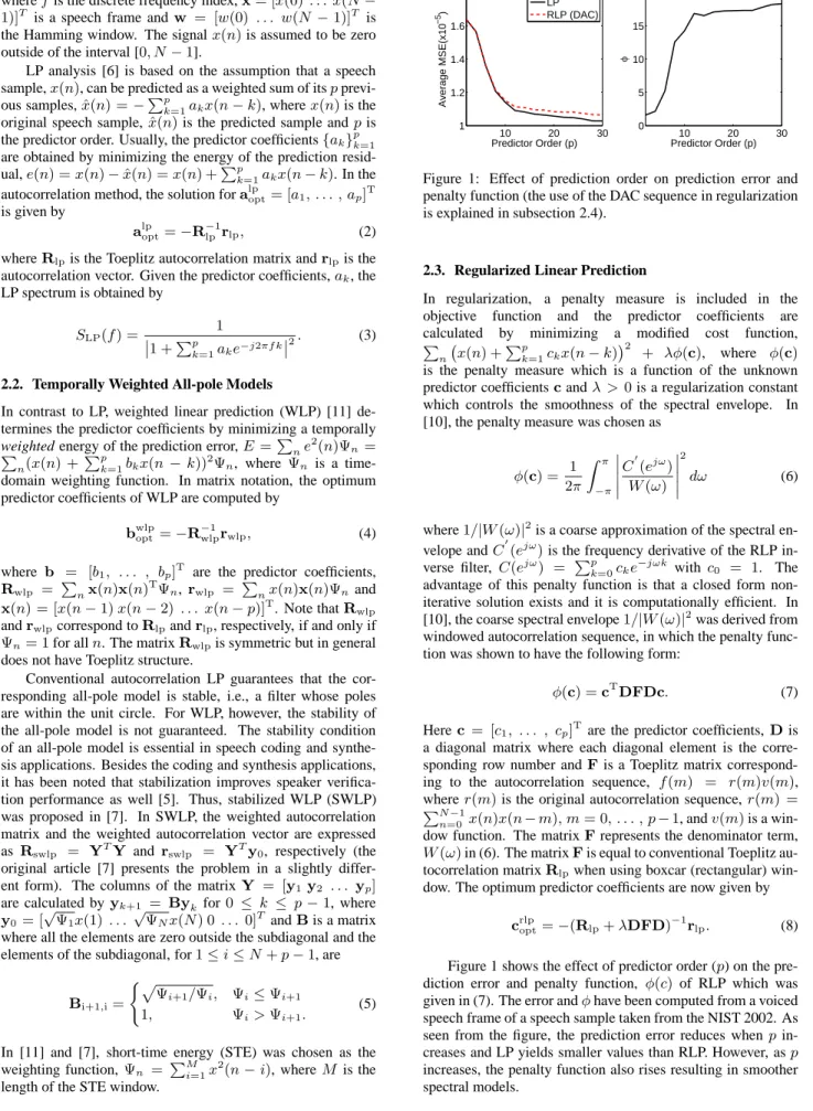
10 20 30 1 1.2 1.4 1.6 1.8 Predictor Order (p) Average MSE(x10 −5 ) LP_{RLP (DAC)} 10 20 30 0 5 10 15 20 Predictor Order (p) φ

Figure 1: Effect of prediction order on prediction error and penalty function (the use of the DAC sequence in regularization is explained in subsection 2.4).

2.3. Regularized Linear Prediction

In regularization, a penalty measure is included in the objective function and the predictor coefficients are calculated by minimizing a modified cost function,

P n x(n) + Pp k=1ckx(n−k) 2 + λφ(c), where φ(c)

is the penalty measure which is a function of the unknown predictor coefficientscandλ > 0is a regularization constant which controls the smoothness of the spectral envelope. In [10], the penalty measure was chosen as

φ(c) = 1 2π Z π −π C′(ejω₎ W(ω) 2 dω (6) where1/|W(ω)|2

is a coarse approximation of the spectral en-velope andC′(ejω_{)is the frequency derivative of the RLP} in-verse filter, C(ejω) = Pp

k=0cke−

jωk

with c0 = 1. The

advantage of this penalty function is that a closed form non-iterative solution exists and it is computationally efficient. In [10], the coarse spectral envelope1/|W(ω)|2

was derived from windowed autocorrelation sequence, in which the penalty func-tion was shown to have the following form:

φ(c) =cTDFDc. (7)

Herec = [c1, . . . , cp]Tare the predictor coefficients, Dis a diagonal matrix where each diagonal element is the corre-sponding row number andFis a Toeplitz matrix correspond-ing to the autocorrelation sequence, f(m) = r(m)v(m), wherer(m)is the original autocorrelation sequence,r(m) =

PN−1

n=0x(n)x(n−m), m= 0, . . . , p−1, andv(m)is a

win-dow function. The matrixFrepresents the denominator term,

W(ω)in (6). The matrixFis equal to conventional Toeplitz au-tocorrelation matrixRlpwhen using boxcar (rectangular)

win-dow. The optimum predictor coefficients are now given by

crlpopt=−(Rlp+λDFD)−1rlp. (8)

Figure 1 shows the effect of predictor order (p) on the pre-diction error and penalty function, φ(c) of RLP which was given in (7). The error andφhave been computed from a voiced speech frame of a speech sample taken from the NIST 2002. As seen from the figure, the prediction error reduces whenp in-creases and LP yields smaller values than RLP. However, asp

increases, the penalty function also rises resulting in smoother spectral models.

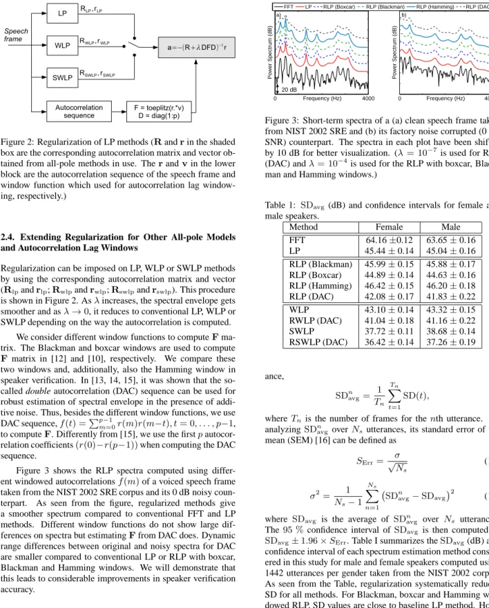
Figure 2: Regularization of LP methods (Randrin the shaded box are the corresponding autocorrelation matrix and vector ob-tained from all-pole methods in use. Therandvin the lower block are the autocorrelation sequence of the speech frame and window function which used for autocorrelation lag window-ing, respectively.)

2.4. Extending Regularization for Other All-pole Models and Autocorrelation Lag Windows

Regularization can be imposed on LP, WLP or SWLP methods by using the corresponding autocorrelation matrix and vector (Rlpandrlp;Rwlpandrwlp;Rswlpandrswlp). This procedure

is shown in Figure 2. Asλincreases, the spectral envelope gets smoother and asλ→0, it reduces to conventional LP, WLP or SWLP depending on the way the autocorrelation is computed.

We consider different window functions to computeF ma-trix. The Blackman and boxcar windows are used to compute

F matrix in [12] and [10], respectively. We compare these two windows and, additionally, also the Hamming window in speaker verification. In [13, 14, 15], it was shown that the so-called double autocorrelation (DAC) sequence can be used for robust estimation of spectral envelope in the presence of addi-tive noise. Thus, besides the different window functions, we use DAC sequence,f(t) =Pp−1

m=0r(m)r(m−t), t= 0, . . . , p−1,

to computeF. Differently from [15], we use the firstp autocor-relation coefficients(r(0)−r(p−1))when computing the DAC sequence.

Figure 3 shows the RLP spectra computed using differ-ent windowed autocorrelationsf(m)of a voiced speech frame taken from the NIST 2002 SRE corpus and its 0 dB noisy coun-terpart. As seen from the figure, regularized methods give a smoother spectrum compared to conventional FFT and LP methods. Different window functions do not show large dif-ferences on spectra but estimatingFfrom DAC does. Dynamic range differences between original and noisy spectra for DAC are smaller compared to conventional LP or RLP with boxcar, Blackman and Hamming windows. We will demonstrate that this leads to considerable improvements in speaker verification accuracy.

2.5. Dynamic Range of the Spectrum Estimators

To compare different spectrum estimators in terms of spectral dynamics (SD), letSD(t) = maxf(20×log10(S(f, t)))−

minf(20×log10(S(f, t)))be theSDoftth speech frame in

decibels (dB). Here,S(f, t)is the estimated magnitude spec-trum of thetth speech frame andfdenotes the frequency bin. LetSDn

avgbe the average spectral dynamics for thenth

utter-0 Frequency (Hz) 4000

Power Spectrum (dB)

0 Frequency (Hz) 4000

Power Spectrum (dB)

FFT LP RLP (Boxcar) RLP (Blackman) RLP (Hamming) RLP (DAC)

a) b)

20 dB

Figure 3: Short-term spectra of a (a) clean speech frame taken from NIST 2002 SRE and (b) its factory noise corrupted (0 dB SNR) counterpart. The spectra in each plot have been shifted by 10 dB for better visualization. (λ= 10−7_{is used for RLP}

(DAC) andλ= 10−4_{is used for the RLP with boxcar,}

Black-man and Hamming windows.)

Table 1: SDavg (dB) and confidence intervals for female and

male speakers.

Method Female Male

FFT 64.16±0.12 63.65±0.16 LP 45.44±0.14 45.04±0.16 RLP (Blackman) 45.99±0.15 45.88±0.17 RLP (Boxcar) 44.89±0.14 44.63±0.16 RLP (Hamming) 46.42±0.15 46.20±0.18 RLP (DAC) 42.08_±0.17 41.83_±0.22 WLP 43.10±0.14 43.32±0.15 RWLP (DAC) 41.04±0.18 41.16±0.22 SWLP 37.72±0.11 38.68±0.14 RSWLP (DAC) 36.42_±0.14 37.26_±0.19 ance, SDnavg= 1 Tn Tn X t=1 SD(t), (9)

whereTnis the number of frames for thenth utterance. By analyzingSDnavg overNs utterances, its standard error of the mean (SEM) [16] can be defined as

SErr= σ √ Ns (10) σ2₌ 1 Ns−1 Ns X n=1 SDnavg−SDavg 2 (11)

where SDavg is the average of SDnavg over Ns utterances. The95 %confidence interval ofSDavg is then computed as

SDavg±1.96×SErr. Table I summarizes theSDavg(dB) and

confidence interval of each spectrum estimation method consid-ered in this study for male and female speakers computed using 1442 utterances per gender taken from the NIST 2002 corpus. As seen from the Table, regularization systematically reduces SD for all methods. For Blackman, boxcar and Hamming win-dowed RLP, SD values are close to baseline LP method. How-ever, when the DAC sequence is used for regularization SD re-duction is larger than conventional methods.

3. Speaker Verification Setup

Speaker recognition experiments are carried out on the NIST 2002 SRE corpus which consists of conversational telephone speech sampled at 8 kHz and transmitted over different cellular

networks. It involves330target speakers (139males and191

females) and39259verification trials (2982targets and36277

impostors). For each target speaker, approximately two minutes of training data is available whereas duration of the test utter-ances varies between 15 seconds and 45 seconds.

Gaussian mixture model with the universal background model (GMM-UBM) [2] is used as the classifier. Test normal-ization (Tnorm) [4] is applied on the log-likelihood scores for score normalization. Two gender-dependent background mod-els and cohort modmod-els for Tnorm with512Gaussians are trained using the NIST 2001 SRE corpus.

Power spectral subtraction (as described in [17]) is used as a pre-processing step in the signal domain to suppress additive noise. The MFCC features are extracted from30ms Hamming windowed speech frames every15ms. Magnitude spectrum es-timation method differs depending on the method. Our baseline system uses the FFT magnitude spectrum of windowed frames. For all-pole methods and their regularized versions, the pre-dictor coefficients and short-time spectra are computed as de-scribed in Section II. All the all-pole methods usep = 20as in [5]. WLP and SWLP are computed as in [5] by utilizing the STE window function withM = 20. The regularization factor

λis10−7_,10−10_and10−10_{in RLP, RWLP, and RSWLP,}

re-spectively. For the Blackman, boxcar and Hamming windowed RLP the regularization factorλis fixed to10−4_{. Theλvalue}

for each method was optimized based on the smallest equal er-ror rate criterion on clean data.

The spectra are processed through a 27-channel triangu-lar filterbank and logarithmic filterbank outputs are converted into MFCCs using the discrete cosine transform (DCT). Af-ter RASTA filAf-tering the 12 MFCCs, their first and second or-der time or-derivatives (∆and∆∆) are appended. The last two steps are energy-based voice activity detector (VAD) followed by cepstral mean and variance normalization (CMVN).

As the performance criteria, we consider both equal error rate (EER) and minimum detection cost function (MinDCF). EER is the threshold value at which false alarm rate (Pfa) and

miss rate (Pmiss) are equal and MinDCF is the minimum value

of a weighted cost function which is given by0.1×Pmiss+

0.99×Pfa. Detection error tradeoff (DET) curves are also

pre-sented to show full behavior of the proposed methods. For additive noise contamination, we use factory2 (which we refer to as ”factory noise”) and babble noises from NOISEX-921. Contaminating the utterances, we add noise sig-nalywith the same length as speech signal asxnoisy=x+Gy in whichGis a gain depends on the desired SNR level. The gain

Gis a single value for the whole utterance and we have not con-sidered any VAD decisions here. The resultantxnoisyis then re-sclaed to have the same scale asx. In the noisy experiments, the target speaker models, background models and Tnorm cohort models are trained using the original data and noise is added to test samples with five different average segmental signal-to-noise-ratios (SNRs): SNR ∈ {clean,20,10,0,−10} dB, where clean refers to the original NIST samples.

3.1. Optimization of the Regularization Parameterλ

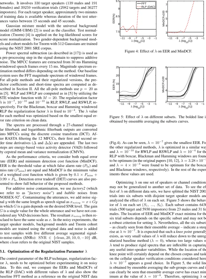
The control parameter of the RLP technique, regularization fac-torλ, needs to be optimized before experimenting it on noisy data. To this end, we compare the EERs and MinDCFs of the RLP (DAC) with different values ofλand also show the baseline FFT method as a reference on the original NIST data

1_{http://www.speech.cs.cmu.edu/comp.speech/Section1/Data/noisex.html} −11 −9 −7 −5 −3 −1 7.5 8 8.5 9 9.5 λ (log₁₀(λ)) EER(%) FFT RLP (DAC) −11 −9 −7 −5 −3 −1 3 4 5 6 7 λ (log₁₀(λ)) MinDCFx100

Figure 4: Effect ofλon EER and MinDCF.

−11 −9 −7 −5 −3 −1 5 10 15 20 25 λ (log₁₀(λ)) EER (%) −11 −9 −7 −5 −3 −1 2 4 6 8 λ (log₁₀(λ)) MinDCFx100

Figure 5: Effect ofλon different subsets. The bolded line is obtained by ensemble averaging the subsets curves.

(Fig.4). As can be seen,λ= 10−7_{gives the smallest EER. For}

the other regularized methods,λis optimized in a similar way andλ= 10−10_{for RWLP and RSWLP andλ= 10}−4_{for the}

RLP with boxcar, Blackman and Hamming windows are found to be optimum (in the original papers [10, 12],λ= 3.28×10−3

andλ = 4×10−3 _{were found to be optimum for the boxcar}

and Blackman windows, respectively). In the rest of the exper-iments these values are used.

Optimizingλon one set of speakers or channel conditions may not be generalized to another set of data. To see the ef-fect ofλon different data sets, we have splitted the NIST 2002 trials into six subsets with disjoint target speaker models and analyzed the effect ofλon each set. Figure 5 shows the behav-ior ofλon each set(S1, ..., S6). Each subset contains 6430

trials (500 target and 5930 impostors) from 23 males and 31 fe-males. The location of EER and MinDCF exact minima for the six trial subsets depends on the specific subset and may not be a robust criterion for settingλ. Nevertheless, all the six subsets – as clearly seen from their ensemble average – indicate a steep rise atλ≈10−7_{.It is expected that such a knee point generally}

exists, as very small values ofλwill reduce down to the unreg-ularized baseline method (λ= 0), wheras too large values of

λtend to produce rigid spectra that are inflexible in capturing any useful inter-speaker variabilities. While the location of the knee point will certainly depend on the chosen corpus and task, on the cellular speaker verification conditions considered here,

λ ≈ 10−7 _{appears a good choice. In Figure 5, the solid line}

is obtained by ensemble averaging the sub-groups curves and it can clearly be seen that ensemble average curve has exact min-imum at the value ofλ = 10−8_{. Therefore, optimizingλon}

one subset and applying it to another subset gives performance close to the optimum.

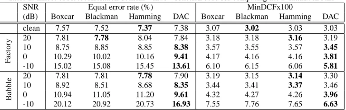
Table 2: Effect of Autocorrelation domain window function used for computing theFmatrix in RLP

SNR Equal error rate (%) MinDCFx100

(dB) Boxcar Blackman Hamming DAC Boxcar Blackman Hamming DAC clean 7.57 7.52 7.37 7.38 3.07 3.02 3.03 3.03 F ac to ry 20 7.81 7.78 8.04 7.84 3.18 3.18 3.16 3.19 10 8.75 8.85 8.85 8.38 3.57 3.55 3.57 3.45 0 10.29 10.02 10.16 9.41 4.17 4.16 4.16 3.81 -10 15.02 15.08 15.45 13.61 6.10 6.15 6.06 5.81 B ab b le 20 7.81 7.81 7.78 7.90 3.19 3.15 3.14 3.30 10 8.92 8.51 8.68 8.35 3.44 3.41 3.37 3.46 0 10.94 11.05 11.20 9.61 4.32 4.27 4.26 3.96 -10 20.12 20.92 20.73 16.93 7.55 7.76 7.65 6.63

Table 3: Speaker recognition performance under additive noise (the DAC sequence is used for regularized methods). For a given noise type and SNR level, all the differences are statistically significant with 95% confidence according to McNemar’s test.

SNR Equal error rate (%) MinDCFx100

(dB) FFT LP RLP WLP RWLP SWLP RSWLP FFT LP RLP WLP RWLP SWLP RSWLP clean 7.65 7.44 7.38 7.48 8.10 7.81 7.94 3.07 3.05 3.03 2.99 3.33 3.08 3.41 F ac to ry 20₁₀ 8.08_9.32 7.83_8.50 7.84_8.38 7.81_8.79 7.75_8.32 8.22_{9.11 8.50}7.85 _3.643.25 _3.563.22 _3.453.19 _3.573.12 _3.323.14 _3.623.21 3.24_3.45 0 10.46 9.93 9.41 10.34 9.62 10.06 9.59 4.13 4.21 3.81 4.19 3.92 4.17 3.92 -10 15.35 14.96 13.61 15.19 13.86 14.35 13.32 6.63 6.14 5.81 6.19 6.03 5.94 5.87 B ab b le 20₁₀ 7.83_8.85 7.78_8.58 7.90_8.35 7.71_8.70 8.21_8.48 8.11_{8.78 8.65}8.17 _3.443.14 _3.483.12 _3.463.30 _3.463.09 _3.533.35 _3.563.19 3.44_3.64 0 11.62 11.23 9.61 11.47 10.29 10.93 9.99 4.53 4.34 3.96 4.49 4.35 4.38 4.27 -10 21.27 20.35 16.93 21.02 18.40 19.69 17.64 8.05 7.67 6.63 7.90 7.22 7.65 7.04

4. Speaker Verification Results

We first examine the effect of different window functions,

v(m), to compute F matrix in RLP method as described in Section 2. The EER and MinDCF values for different window functions are given in Table 2. As seen from the table, different window functions do not show large differences on recognition accuracy as expected from Figure 3 and Table 1. However, us-ing the DAC sequence to computeFmatrix improves recogni-tion accuracy extensively.

Next, we analyze regularization of the temporally weighted all-pole methods, RWLP and RSWLP, using the DAC sequence. The results are given in Table 3. Figure 6 shows the DET plots of each regularized and unregularized all-pole method in com-parison to the baseline FFT method for babble noise at SNR level of -10 dB. Recognition accuracy of all methods degrades under additive noise as expected. The following observations can be made:

• In clean condition, LP, RLP and WLP methods slightly outperform the baseline FFT technique.

• For factory noise contamination, RLP outperforms other methods at low SNR levels (0 dB and -10 dB). RWLP and RSWLP show minor improvements over all-pole methods at high SNR levels (20 dB and 10 dB). In terms of MinDCF, RLP outperforms the other methods at low SNRs (0 dB and -10 dB) while RWLP wins at high SNRs (10 dB and 20 dB)

• For babble noise, RLP achieves the smallest EER in nearly all cases (WLP is slightly better at 20dB). In terms of MinDCF, WLP gives smaller MinDCF values at high SNR levels. In the noisier cases, RLP yields the smallest values among the other methods.

4.1. Effect of Regularization on Different Conditions

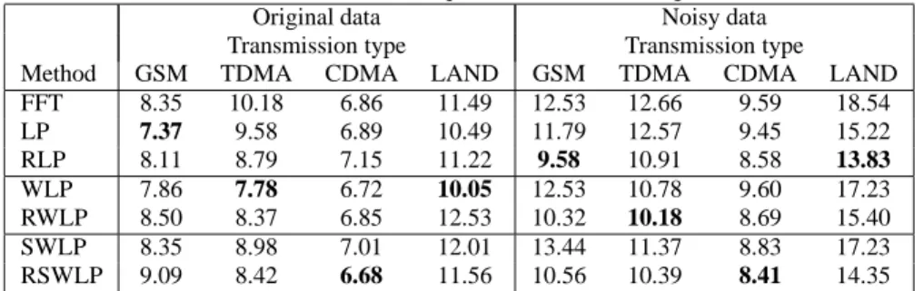
It was shown in the previous section that improvement on recog-nition accuracy by regularization is significant. However, one may argue that the improvement may depend on how the speech samples are represented and transmitted, since NIST 2002 con-sists of various telephony data. To gain insight into the poten-tial impact of transmission type, we have broken down NIST 2002 verification trials into different subsets with respect to transmission types. NIST 2002 corpus consists of telephone speech recorded using four different transmission types: GSM (Global System for Mobile communications), TDMA (Time Di-vision Multiple Access), CDMA (Code DiDi-vision Multiple Ac-cess), and LANDLINE as specified in the database.

We have compared baseline spectrum estimation methods with regularized ones using original NIST data and under bab-ble noise condition (0 dB SNR). Tabab-ble 4 summarizes the num-ber of target and impostor trials for each transmission system. Table 5 shows the EERs (%) for different transmission types un-der original and noisy conditions. In the clean case, baseline LP gives the smallest EER value for the GSM data whereas WLP is the best choice for the TDMA and LANDLINE conditions. RSWLP outperforms the other methods for the CDMA. In the noisy case, regularized methods are superior to the baseline techniques for all transmission types. RLP shows promising performance for GSM and LANDLINE data. For the TDMA and CDMA conditions, the smallest EERs are obtained using RWLP and RSWLP, respectively. In the noisy case, the relative improvements over the baseline methods are considerably high. In general, the recognition performance of regularized methods is better than the conventional ones in noisy case for all trans-mission types.

Unfortunately, no transmission details are provided in the database except for the fact that the first three of these standards are wireless and the last one is the conventional wired

2 5 10 20 40 2 5 10 20 40

False Alarm probability (in %)

Miss probability (in %)

FFT (EER:21.28% MinDCF:8.05) LP (EER:20.36% MinDCF:7.67) RLP (EER:16.93% MinDCF:6.73) NIST 2002 babble noise, −10 dB SNR 2 5 10 20 40 2 5 10 20 40

False Alarm probability (in %)

Miss probability (in %)

FFT (EER:21.28% MinDCF:8.05) WLP (EER:21.02% MinDCF:7.90) RWLP (EER:18.40% MinDCF:7.22) NIST 2002, babble noise, −10 dB SNR 2 5 10 20 40 2 5 10 20 40

False Alarm probability (in %)

Miss probability (in %)

FFT (EER:21.28% MinDCF:8.05) SWLP (EER:19.69% MinDCF:7.65) RSWLP (EER:17.64% MinDCF:7.04)

NIST 2002, babble noise, −10 dB SNR

Figure 6: DET plots for different spectrum estimators under -10 dB SNR babble noise (the DAC sequence is used for regularized methods).

Table 4: Number of target and impostor trials of each sub-condition for transmission types.

Number of Transmission type

trials GSM TDMA CDMA LAND Total target 407 167 1312 383 2269 impostor 4092 1934 14583 7713 28322 Total 4499 2101 15895 8096 30591

sion. However, one can assess the effect of different transmis-sion types on recognition performance only in general terms. The parameters that may affect the recognition performance are bit error rates and speech compression type, as they may alter the original speech spectrum. Since the bit error rate perfor-mance of CDMA transmission is better than the other two due to the nature of its signaling format, it yields the lowest EER in all cases (clean and noisy). The reason of yielding highest EER in the case of LANDLINE transmission in all cases com-pared to the wireless transmissions is the fact that the channel effects are compensated for by adaptive channel equalization in wireless systems in contrast to the LANDLINE transmission.

5. Conclusion

Regularization of all-pole models was studied for robust speaker verification. The regularized all-pole methods outper-formed standard FFT and LP techniques under two different additive noise types, factory and babble noises. In general, reg-ularization using the DAC sequence yielded considerable im-provement on the recognition performance especially at low SNRs for conventional and temporally weighted all-pole meth-ods. It was also shown that recognition accuracy depends on the transmission type used and regularization improves the verifica-tion performance for different transmission types. In summary, the regularized LP based spectrum estimation holds promise for speaker verification in noisy conditions. Adaptive selection ofλ

based on estimated SNR level or fundamental frequency (as in [10]) is a potential area of future studies. Analyzing the perfor-mance of RLP method with a more recent corpus and modeling algorithm (e.g. NIST 2010 and i-vector system) would also be interesting.

6. Acknowledgement

The work of C. Hanilc¸i was supported by Turkish Council of Higher Education. The work of T. Kinnunen and J. Pohjalainen were supported by Academy of Finland (projects 132129 and

127345). The work of Rahim Saeidi was funded by the Euro-pean Community’s seventh framework programme (FP7/2007-2013) under grant agreement no. 238803.

7. References

[1] T. Kinnunen and H. Li, “An overview of text-independent speaker recognition: from features to supervectors,” Speech Comm., vol. 52, no. 1, pp. 12–40, Jan. 2010. [2] D.A. Reynolds, T.F. Quatieri, and R.B. Dunn, “Speaker

verification using adapted Gaussian mixture models,” Dig. Sig. Proc., vol. 10, no. 1, pp. 19–41, Jan. 2000.

[3] P. Kenny, G. Boulianne, P. Ouellet, and P. Dumochel, “Joint factor analysis versus eigenchannels in speaker recognition,” IEEE Trans. Audio, Speech and Lang. Proc., vol. 15, no. 4, pp. 1435–1447, May 2007.

[4] R. Auckenthaler, M. Carey, and H. Lloyd-Thomas, “Score normalization for text-independent speaker verification systems,” Dig. Sig. Proc., vol. 10, no. 1-3, pp. 42–54, Jan. 2000.

[5] R. Saeidi, J. Pohjalainen, T. Kinnunen, and P. Alku, “Tem-porally weighted linear prediction features for tackling ad-ditive noise in speaker verification,” IEEE Sig. Proc. Lett., vol. 17, no. 6, pp. 599–602, June 2010.

[6] J. Makhoul, “Linear prediction: a tutorial review,” Proc. of the IEEE, vol. 64, no. 4, pp. 561–580, Apr. 1975. [7] C. Magi, J. Pohjalainen, T. B¨ackstr¨om, and P. Alku,

“Sta-bilized weighted linear prediction,” Speech Comm., vol. 51, no. 5, pp. 401–411, April 2009.

[8] C. Hanilc¸i, T. Kinnunen, F. Ertas¸, R. Saeidi, J. Poh-jalainen, and P. Alku, “Regularized all-pole models for speaker verification under noisy environments,” IEEE Sig. Proc. Lett., vol. 19, no. 3, pp. 163–166, March 2012. [9] Trevor Hastie, Robert Tibshirani, and Jerome Friedman,

The Elements of Statistical Learning, Springer Series in Statistics. Springer New York Inc., New York, NY, USA, 2001.

[10] L. A. Ekman, W. B. Kleijn, and M. N. Murthi, “Regu-larized linear prediction of speech,” IEEE Trans. Audio, Speech and Lang. Proc., vol. 16, no. 1, pp. 65–73, Jan. 2008.

[11] C. Ma, Y. Kamp, and L. Willems, “Robust signal selection for linear prediction analysis of voiced speech,” Speech Comm., vol. 12, no. 1, pp. 69–81, March 1993.

Table 5: Comparison of the baseline FFT and LP methods with RLP in terms of EER (%) for different transmission conditions using original and noisy data with 0 dB SNR babble noise (the DAC sequence is used for all regularized methods).

Original data Noisy data Transmission type Transmission type

Method GSM TDMA CDMA LAND GSM TDMA CDMA LAND FFT 8.35 10.18 6.86 11.49 12.53 12.66 9.59 18.54 LP 7.37 9.58 6.89 10.49 11.79 12.57 9.45 15.22 RLP 8.11 8.79 7.15 11.22 9.58 10.91 8.58 13.83 WLP 7.86 7.78 6.72 10.05 12.53 10.78 9.60 17.23 RWLP 8.50 8.37 6.85 12.53 10.32 10.18 8.69 15.40 SWLP 8.35 8.98 7.01 12.01 13.44 11.37 8.83 17.23 RSWLP 9.09 8.42 6.68 11.56 10.56 10.39 8.41 14.35

[12] M. N. Murthi and W. B. Kleijn, “Regularized linear pre-diction all-pole models,” in IEEE Speech Coding Work-shop, 2000, pp. 96–98.

[13] D. Mansour and B.H. Juang, “The short-time modified coherence representation and noisy speech recognition,” IEEE Trans. Acoust. and Sig. Proc., vol. 37, no. 6, pp. 795–804, Jan. 1989.

[14] T. Shimamura and N. D. Nguyen, “Autocorrelation and double autocorrelation based spectral representations for a noisy word recognition systems,” in Interspeech, 2010, pp. 1712–1715.

[15] H. Kobatake and Y. Matsunoo, “Degraded word recogni-tion based on segmental signal-to-noise ratio weighting,” in ICASSP, 1994, pp. 425–428.

[16] X. Huang, A. Acero, and H.-W. Hon, Spoken Language Processing: A Guide to Theory, Algorithm and System De-velopment, Prentice Hall, 2001.

[17] P. C. Loizou, Speech Enhancement: Theory and Practice, CRC Press, 2007.

A. MATLAB CODE FRAGMENT OF

STANDARD WINDOWED RLP

The following matlab code of the regularized LP spectrum esti-mator using windowed autocorrelation sequence studied in this paper. The inputs of the function are the speech signalx, regu-larization factorλand the window type ”win” used to window autocorrelation sequence. The function itself reduces to method proposed in [10] when win=’boxcar’ is used.

function spectrum = rlp_win(x,lambda,win)

% This function computes the RLP spectrum using % windowed autocorrelation sequence of a given % speech signal x and regularization factor lambda % NOTE: the function reduces to the method proposed in % Ekman et. al. 2008 when 'boxcar' is used as window.

p=20; % LP predictor order

nfft = 512;

frames = buffer(x,240,120,'nodelay');

frames = bsxfun(@times,frames,hamming(240)); switch(win) case{'boxcar'} wfunc = ones(p,1); case{'hamming'} wfunc = hamming(p); case{'blackman'} wfunc = blackman(p); end % Biased autocorrelation X = fft(frames,nfft); R = ifft(abs(X).ˆ2); R = R./size(frames,1); a = zeros(p+1,size(R,2)); D = diag(1:p); for i = 1:size(R,2) r = R(2:p+1,i); Autocorr = toeplitz(R(1:p,i)); % Windowed autocorrelation F = toeplitz(R(1:p,i).*wfunc); a2 = (Autocorr+lambda*D*F*D)\r; a(:,i) = [1;-a2]; end

% Inverse filter spectrum

ifspec = 1./abs(fft(a,nfft)).ˆ2; spectrum = ifspec(1:nfft/2+1,:);

B. MATLAB CODE FRAGMENT OF RLP

WITH DAC SEQUENCE

The matlab code of the proposed regularization of the all-pole models using DAC sequence is given below. The inputs of the function are the speech signalxand the regularization factorλ.

function spectrum = rlp_dac(x,lambda)

% This function computes the RLP spectrum using % DAC sequence of a given speech signal x and % regularization factor lambda

p=20; % LP predictor order

nfft = 512;

frames = buffer(x,240,120,'nodelay');

frames = bsxfun(@times,frames,hamming(240)); % Biased autocorrelation X = fft(frames,nfft); R = ifft(abs(X).ˆ2); R = R./size(frames,1); a = zeros(p+1,size(R,2)); D = diag(1:p); for i = 1:size(R,2) r = R(2:p+1,i); Autocorr = toeplitz(R(1:p,i)); % DAC sequence

Autocov = xcov(R(1:p,i),'coeff');

Autocov = Autocov(p:2*p-1); F = toeplitz(Autocov(1:p)); a2 = (Autocorr+lambda*D*F*D)\r; a(:,i) = [1;-a2];

end

% Inverse filter spectrum

ifspec = 1./abs(fft(a,nfft)).ˆ2; spectrum = ifspec(1:nfft/2+1,:); end