Working Paper n° 08-02
Fourth Order Pseudo Maximum
Likelihood Methods
Alberto Holly, Alain Monfort and
Michael Rockinger
Fourth Order Pseudo Maximum
Likelihood Methods
Alberto Holly
1, Alain Monfort
2and
Michael Rockinger
31
Institute of Health Economics and
Management(IEMS), University of Lausanne, Faculty of Business and Economics, Extranef Building, CH-1015 Lausanne, Switzerland.
E-mail: [email protected]
2
Corresponding author. CNAM and CREST, 15 Boulevard Péri, 92245 Malakoff Cédex, France.
E-mail: [email protected]
3
Swiss Finance Institute and CEPR, University of Lausanne, Faculty of Business and Economics, Extranef Building, CH-1015 Lausanne,
Switzerland.
E-mail: [email protected]
This text is not to be cited without the permission of the authors.
Working Paper n° 08-02
Fourth Order Pseudo Maximum
Likelihood Methods
by Alberto Holly
a, Alain Monfort
b,
and Michael Rockinger
cAugust 2008
aInstitute of Health Economics and Management (IEMS), University of Lausanne, Faculty of Business and Economics, Extranef Building, CH-1015 Lausanne, Switzerland. E-mail: [email protected].
b Corresponding author. CNAM and CREST, 15 Boulevard P´eri, 92245 Malakoff C´edex, France, E-mail: [email protected].
c Swiss Finance Institute, University of Lausanne, and CEPR. University of Lausanne. Faculty of Business and Economics, Extranef Building, CH-1015 Lausanne, Switzerland. E-mail: [email protected].
Acknowledgement: The third author acknowledges support from the Swiss National Sci-ence Foundation through NCCR FINRISK (Financial Valuation and Risk Management). We are grateful to Prof. W. Gautschi for his advice concerning numerical integration and to Prof. G. V. Milovanovi´c for providing a very useful sequence of parameters used for numeri-cal integrations.
Keywords: Quartic Exponential Family, Pseudo Maximum Likelihood, Skew-ness, Kurtosis.
Abstract
The objective of this paper is to extend the results on Pseudo Maximum Like-lihood (PML) theory derived in Gourieroux, Monfort, and Trognon (GMT) (1984) to a situation where the first four conditional moments are specified. Such an extension is relevant in light of pervasive evidence that conditional dis-tributions are non-Gaussian in many economic situations. The key statistical tool here is the quartic exponential family, which allows us to generalize the PML2 and QGPML1 methods proposed in GMT(1984) to PML4 and QGPML2 methods, respectively. An asymptotic theory is developed which shows, in par-ticular, that the QGPML2 method reaches the semi-parametric bound. The key numerical tool that we use is the Gauss-Freud integration scheme which solves a computational problem that has previously been raised in several econometric fields. Simulation exercises show the feasibility and robustness of the methods.
1. Introduction
It is well known that the Maximum Likelihood estimator may not only be inefficient but also inconsistent under misspecification. Specifically, this oc-curs when the parametric model providing the likelihood function does not contain the true distribution. The study of the relations between Maximum
Likelihood Theory and misspecification has now a long history. Hood and
Koopmans (1953) demonstrated that the conditionally Gaussian ML estimator is consistent and asymptotically Gaussian, even if the true distribution is not conditionally Gaussian, as soon as the first two conditional moments are well specified. They coined the label “quasi ML estimator” for this kind of esti-mator. White (1982) showed that, under misspecification, the ML estimator is in fact a CAN (consistent asymptotically normal) estimator of the pseudo-true value (as defined for instance in Sawa (1978)). Gourieroux, Monfort, and Trognon (1984) characterized the parametric families leading to CAN estima-tors of the parameters appearing in the first two conditional moments, even if the true distribution does not belong to this parametric family. These families are the linear exponential families (when only the first conditional moment is specified) and the quadratic exponential families (when the first two conditional moments are specified). The estimators thus obtained were called PML1 and PML2 estimators, respectively. Bollerslev and Wooldrige (1992) generalized the properties of the quasi generalized estimator, i.e. the Gaussian PML estimator, to the dynamic case.
The PML theories described above only consider the robustness of the estima-tor of the parameters appearing in the first two conditional moments. More re-cently, however, many econometric fields are paying greater attention to higher order conditional moments. This is particularly the case, in Financial Econo-metrics and in Health EconoEcono-metrics. Very often, the approach used to account for higher moments is the ML method based on a choice of a parametric family, which allows for asymmetry and fat tails. A few such examples, occurring in finance are: Generalized Hyperbolic distribution [Eberlein and Keller (1995); Barndorff-Nielsen (1997)], the noncentral Student t distribution [Harvey and Siddique (1999)], and the Skewed-t distribution [Hansen (1994); Jondeau and
Rockinger (2003)]. In Health Econometrics, some examples are: The Gener-alized Gamma distribution proposed by Stacy (1962) and Stacy and Mihram (1965), [Manning, Basu, and Mullahy (2005)], and the Pearson Type IV dis-tribution, which may be considered a skewed-t distribution [Holly and Pentsak (2004)]. More generally, examples can be found in various fields, including physics, astronomy, image processing, and in the biomedical sciences [see Gen-ton (2004) and Arellano-Valle and GenGen-ton (2005)].
Current ML approaches have two types of drawbacks. First, some families may not be flexible enough to span the whole set of possible skewness (s) and kurtosis (k), namely the domaink ≥s2+1.Second, as mentioned above, the risk
of misspecification may lead to inconsistent estimators. If we are interested in the first four conditional moments, a natural method is the Generalized Method of Moments (GMM). There is now a large body of studies, however, suggesting that GMM estimators can have poor finite sample properties [see e.g. Tauchen (1986), Andersen and Sorenson (1996), Altonji and Segal (1996), Ziliak (1997), Doran and Schmidt (2006)]. These difficulties led Kitamura and Stutzer (1997), relatively early on, to propose an alternative estimation procedure based on the Kullback-Leibler Information Criterion.
The objective of this paper is to propose another alternative to GMM. It is an extension of the PML method developed by Gourieroux, Monfort, and Trognon (1984), henceforth referred to as GMT. This work extends GMT to a situation where the first four moments (centered or not) are known functions depend-ing on unknown parameters. Specifically, we show that the PML estimator is consistent for any specification of the first four conditional moments, any true conditional distribution of the endogenous variable, and any marginal distribu-tion of the exogenous variables, if and only if the PML is based on a quartic exponential family. We shall refer to this extension as PML4. We also propose an extension of the Quasi-Generalized Pseudo Maximum Likelihood (QGPML) estimator proposed by GMT (1984) based on the quartic exponential family. We show that this estimator, which we refer to as QGPML2, reaches the semi-parametric bound. Beyond the robustness and nice asymptotic properties of the estimates resulting from the quartic exponential families, two additional features should be noted. First, the quartic exponential family spans the whole domain of the pairs (s, k), except for a set of measure zero. This is not nec-essarily the case for other parametric families of distributions such as those mentioned earlier. Second, we show how the parameters of the quartic expo-nential family may be obtained from a given set of moments. Thereby, we solve
a numerical problem which had been already encountered, both in the econo-metric literature [Zellner and Highfield (1988), Ormoneit and White (1999)] and
other fields [Agmon et al. (1979) or Mead and Papanicolaou (1984)], where the
exponential family arises as an Entropy Maximizing density and which were considered as difficult. The key issue, from the computational point of view, is the use of the Gauss-Freud quadrature scheme which seems very promising for computing the numerical integrations needed in this framework.
The rest of this paper is organized as follows. Preliminary results are given in Section 2, where some properties of exponential families are briefly reviewed and the notion of a quartic exponential family is defined. This section also contains a brief presentation of the properties of M-Estimators. These prelim-inary results are then used to derive important properties of the exponential quartic family in Section 3. The PML4 method is defined in Section 4, and the asymptotic properties of the PML4 estimators are derived. In Section 5, we perform a similar analysis as in Section 4 but for the QGPML2 method. In Section 6, we discuss the numerical issues and describe numerical algorithms for implementing of the PML4 and QGPML2 methods. Several Monte-Carlo exercises demonstrating the usefulness of the methods proposed in our paper are presented in Section 7. This section contains a discussion on computational issues linked with the quartic exponential distribution, and it also presents four Monte-Carlo experiments, each of which numerically demonstrates a different property of PML4 or QGPML2. Conclusions are presented in Section 8. Fi-nally, to not interrupt our discussion of the essential ideas of this paper, some proofs and other technical details are presented in the Appendix.
2. Preliminaries 2.1. Exponential Families.
Let us consider a measure space (Y,A, ν) where A is a σ−field and ν a
σ−finite measure. An exponential family is a family of probability distributions on (Y,A) which are equivalent to ν and with pdfs of the form:
`(y, λ) = exp [λ0T(y)−ψ(λ)], λ∈Λ⊂Rp,
where T(y) is a p−dimensional vector defined onY,and ψ(λ) is a normalizing constant, equal to the Log-Laplace transform of νT, equivalent to the image of
Such families have many well-known properties. Some of them will be useful in the rest of the paper, and they are summarized below [the proofs can be found for instance in Barndorff-Nielsen (1978), Monfort (1982), or Brown (1986)].
(1) Λ can be taken as the convex set where the Laplace transform of νT is
defined.
(2) For any λ ∈ ˚Λ, interior of Λ, all the moments of the statistic T exist, and in particular, we have:
Eλ(T) = ∂ ∂λψ(λ), Vλ(T) = ∂2 ∂λ∂λ0ψ(λ), which implies: ∂Eλ(T) ∂λ0 = ∂2 ∂λ∂λ0ψ(λ) = Vλ(T).
(3) The Fisher information matrixIF(λ) is equal toVλ(T) = ∂2ψ(λ)/∂λ∂λ0.
(4) The model is identifiable if, and only if,IF(λ) is invertible for anyλ ∈Λ.
(5) If the model is identifiable, then the mapping λ→Eλ(T) is injective.
2.2. Quartic Exponential Family.
We consider the particular case whereY =R, A=BR (the Borelianσ−field of R),ν is the Lebesgue measure on R, and T(y) = (y, y2, y3, y4)0.
In other words, we consider the pdfs on R defined by:
`(y, λ) = exp " 4 X i=1 λiyi−ψ(λ) # , with λ= (λ1, λ2, λ3, λ4)0. (2.1)
We will also use the notation:
`(y, λ) = exp " λ0+ 4 X i=1 λiyi # , with λ0 =−ψ(λ). (2.2)
This type of density has been extensively used in the entropy literature, e.g.
Golan et al. (1996), since it is obtained by maximizing, with respect to f,
the entropy−R
Rf(y) logf(y)dy,under a set of data moment-consistency con-straints R
Ry
if(y) dy=m
j,forj = 1,· · · ,4, where themj are given, as well as
a normalization constraintR
Rf (y)dy = 1.
The set Λ where `(y, λ) is defined is easily obtained. If λ4 < 0, `(y, λ) is
always integrable. If λ4 > 0, `(y, λ) is never integrable. Finally, if λ4 = 0,
`(y, λ) is integrable if λ3 = 0 andλ2 <0. In other words, Λ is defined by:
Λ =R×R×R×R−∗+R×R−∗× {0} × {0},
where R−∗ is the set of strictly negative numbers.
This family will be called the quartic exponential family and denoted by
family. Therefore, since on this set, T(y) is integrable, the quartic family is not steep [see Brown (1986), p. 72]. Consequently, we cannot use the standard results developed by Barndorff-Nielsen (1978) about the range of the mapping
λ→Eλ[T(y)] for steep families. For more details, see Barndorff-Nielsen (1978),
Brown (1986), Letac (1992), and Appendix A.
One should note that the variance-covariance matrix ofT(Y) = (Y, Y2, Y3, Y4)0 is invertible everywhere, since otherwise there would exist a linear relation be-tween Y, Y2, Y3, Y4, i.e. the support of the distribution of Y would be made
of at most four points, which is impossible since this distribution is absolutely continuous with respect to the Lebesgue measure. Therefore, using the general properties 3) and 4) we see that the model is identifiable. Moreover, using 5) we conclude that the mapping λ→[mi(λ), i= 1, . . . ,4], where mi(λ) = Eλ(Yi), is
injective.
Denoting bys(λ) andk(λ) the skewness and kurtosis [s(λ) =Eλ[Y−E(Y)]3/
[Vλ(Y)]3/2, k(λ) = Eλ[Y −E(Y)]4/[Vλ(Y)]2], respectively, it is also clear that
the mapping:
λ→[m1(λ), m2(λ), s(λ), k(λ)],
is injective. The same is true for the mapping
λ→[m(λ), σ2(λ), s(λ), k(λ)],
where m(λ) = m1(λ), and σ2(λ) =m2(λ)−m21(λ).
It is important to check whether the previous mapping is also surjective, which is to say that it can reach any admissible value of (m1, m2, s, k). It is
well known that the set D of admissible values of (m, σ2, s, k) is defined by:
m∈R, σ2 ≥0, s∈R, k≥s2+ 1.
The latter inequality is obtained, for instance, by noting that the variance-covariance matrix of (Y, Y2) whereE(Y) = 0, V(Y) = 1, is given by
1 s
s k−1
! ,
and therefore that k − 1−s2 ≥ 0. Moreover, the boundary k = s2 + 1 is
reached if Y and Y2 are linked linearly, that is, if the support is made of at most two points. Therefore, this boundary clearly cannot be reached by the
quartic family, and the boundary point σ2 = 0 cannot be reached either (for
range D of the mappingλ→[m(λ), σ2(λ), s(λ), k(λ)] defined by:
m∈R, σ2 >0, s∈R, k > s2 + 1 ?
The answer is no, but it can be shown [see Junk (2000)] that the range is almost equal to this set, in the sense that all the admissible values of (m, σ2, s, k) can
be reached except for those corresponding to the set of measure zero, defined by s = 0, k > 3. In particular, we can approach all the points of the half line
s= 0, k >3, in the plane (s, k), as closely as we wish.
2.3. M-estimators and Quasi-Generalized M-estimators.
Let us consider an endogenous variableYiand a vector of exogenous variables
Xi. For simplicity, we assume that (Yi, Xi) for i= 1,· · · , n are i.i.d. Standard
extensions can be found in Gallant (1987), Holly (1993), or White (1994). To each possible conditional distribution of the Yi’s given the Xi’s, we associate a
parameterθ ∈Θ⊂RK. In particular, the value of the parameter corresponding
to the true conditional distribution of the Yi’s given the Xi’s is called the true
value of the parameter, and it is denoted by θ0. The true distribution of the
sequence (Yi, Xi, i ∈ N) is denoted by P0. Throughout this paper, we adopt
the notation corresponding to a conditional static model, but the results could
be extended to a stationary conditional dynamic model by replacing Yi by Yt
and Xi by (Yt−1, . . . , Y1, Xt, . . . , X1).
An M-estimator ofθ0 is an estimator ˆθnobtained by maximizing, with respect
toθ, an objective function of the form:
n
X
i=1
ϕ(Yi, Xi, θ). (2.3)
Under standard regularity conditions [see e.g. Chamberlain (1987), Newey
(1990), White (1994), Gourieroux and Monfort (1995a)], it can be shown that ˆ
θn is a consistent estimator of θ0, for any θ0, if the limit function ϕ∞(θ, P0) =
P0lim 1 n Pn i=1ϕ(Yi, Xi, θ)
has a unique maximum at θ = θ0. Moreover, the
limit function can be written:
ϕ∞(θ, P0) = EXE0ϕ(Y, X, θ), (2.4)
where E0 is the conditional expectation operator associated to the true
condi-tional distribution of Yi, given that Xi = x (independent of i) and EX is the
expectation with respect to the distribution PX, of any Xi.
Let us now consider two subvectorsθ∗ andθ∗∗ ofθ. These subvectors are not necessarily disjoint, and in particular, we can have θ∗ =θ∗∗=θ.
We assume thatθ0∗, the true value of θ∗, can be consistently estimated by ˆθn∗ defined by: ˆ θ∗n= Argmax θ∗ n X i=1 ϕhYi, Xi, θ∗, a Xi,θˆ∗∗n i , (2.5)
whereais some function, and ˆθn∗∗is a consistent estimator ofθ∗∗0 , the true value of θ∗∗. In other words, θ∗0 gives the unique maximum in θ∗ of:
P0lim " 1 n n X i=1 ϕhYi, Xi, θ∗, a Xi,θˆ∗∗n i # (2.6) =EXE0ϕ[Y, X, θ∗, a(X, θ0∗∗)]. (2.7)
Such an estimator is called a Quasi-Generalized M-estimator of θ∗0 (QGM esti-mator). The corresponding unfeasible M-estimator ˆθ∗0n is defined by:
ˆ θ∗0n = Argmax θ∗ n X i=1 ϕ[Yi, Xi, θ∗, a(Xi, θ∗∗0 )], (2.8)
and is also consistent.
As far as the asymptotic behavior of the M and QGM estimators is concerned, we have the following properties.
The asymptotic distribution of √n(ˆθn − θ0) is N [0, J−1(θ0)I(θ0)J−1(θ0)]
where J(θ0) =−EXE0 ∂2ϕ(Y, X, θ 0) ∂θ∂θ0 , (2.9) I(θ0) =EXE0 ∂ϕ(Y, X, θ0) ∂θ ∂ϕ(Y, X, θ0) ∂θ0 . (2.10)
A nice property of the QGM-estimator ˆθ∗n of θ0∗ is the following. If
E0 ∂2ϕ(Y, X, θ∗0, a(X, θ0∗∗) ) ∂θ∗∂a0 |X = 0, (2.11)
then√n(ˆθ∗n−θ0∗) has the same asymptotic distribution as√n(ˆθ0∗n−θ0∗). Namely,
Nh0,J˜−1(θ
0) ˜I(θ0) ˜J−1(θ0)
i
,where ˜J(θ0) and ˜I(θ0) are obtained from (2.9) and
(2.10), onceθhas been replaced byθ∗andϕ(Y, X, θ) byϕ(Y, X, θ∗, a(X, θ∗∗0 )).
3. Properties of the Exponential Quartic Family
Let us denote by
`(y, λ) = exp(λ0 +λ1y+λ2y2+λ3y3+λ4y4),
We know that the range Λ of λis: Λ =R3×
R−∗+R×R−∗× {0} × {0},and
let us denote by D the set of the values of (m1, σ2, s, k) which can be reached
by this family. We have seen in Subsection 2.2 that:
D=
m1 ∈R, σ2 >0, s∈R, k > s2+ 1 − {s= 0, k >3}.
Let us denote by M the corresponding range of m = (m1, m2, m3, m4)0, where
mi =E(Yi).
We know from Subsection 2.2 that the mapping m(λ) from Λ to M is
bijec-tive, and we denote by λ(m) the inverse function and λ0(m) =−ψ[λ(m)].
Proposition 1. We have: ∂λ0(m) ∂m + ∂λ0(m) ∂m m= 0. (3.1) Proof. We have: Log`[y, λ(m)] =λ0(m) + 4 X j=1 λj(m)yj, ∂Log`[y, λ(m)] ∂m = ∂λ0(m) ∂m + 4 X j=1 ∂λj(m) ∂m y j.
The result follows by taking the expectation and using the fact that the score
vector is of zero mean.
Corollary 1. We have: ∂2λ 0(m) ∂m∂m0 + 4 X j=1 ∂2λ j(m) ∂m∂m0 mj + ∂λ0(m) ∂m = 0. (3.2)
Proof. The proof is straightforward by differentiating the identity (3.1) of
Propo-sition 1 once more.
Let us denote by Σ the variance-covariance matrix ofT(Y) = (Y, Y2, Y3,Y4)0 which is positive definite (since the support ofY is not reduced to point masses).
Proposition 2. We have ∂m/∂λ0 = Σ, and therefore, ∂λ/∂m0 = Σ−1.
Proof. This is a direct consequence of the general property 2) of Subsection 2.1.
Proposition 3. For any pair m, m0 ∈M, we have:
λ0(m) +λ0(m)m0 ≤λ0(m0) +λ0(m0)m0,
Proof. From Kullback’s inequality, we know that: Em0{Log`[y, λ(m)]} ≤Em0{Log`[y, λ(m0)]}, or Em0[λ0(m) +λ 0(m)T(Y)]≤E m0[λ0(m0) +λ 0(m 0)T(Y)],
and the result follows.
4. PML 4 Method
4.1. Definition.
We adopt a semi-parametric approach based on the specifying of the condi-tional moments up to fourth order. This is obviously equivalent to specifying (m1, m2, m3, m4) or (m1, σ2, s, k). Moreover, to satisfy the inequalityk > s2+1,
it could be convenient to specify (m1, σ2, s, k∗), where k∗ =k−s2 −1, which
could be called the over-kurtosis, since (s, k∗) is only constrained to belong to
R+ ×R+. We consider the latter parametrization, but the results could be
adapted to other parametrizations in a straightforward manner.
We therefore specify the following functions: m(xi, θ1), σ2(xi, θ2), s(xi, θ3),
and k∗(xi, θ4). Note that θ1, θ2, θ3, and θ4 may have some components in
common, and we denote by θ the union of θ1, θ2, θ3, and θ4 without repetition
(in particular, we could have θ1 = θ2 = θ3 = θ4 = θ). We denote by Θ the
range of θ.
For a given xi and θ, we can compute the coefficientsλ0, λ1, λ2, λ3, λ4 of the
quartic exponential distribution having the same mean, variance, skewness and kurtosis. As mentioned in Section 2, this can always be done unless the skewness is zero and the kurtosis larger than 3, but even then these values can be closely approached. Let us denote these coefficients by λj(xi, θ), j = 0, . . . ,4.
Definition 1. The fourth order Pseudo Maximum Likelihood estimator of θ0,
called PML4 and denoted by θˆn is defined by:
ˆ θn= Argmax θ∈Θ n X i=1 4 X j=0 λj(xi, θ)yji.
Condition 1. We assume that the semiparametric model is identifiable, i.e. that:
(1) if m1(xi, θ1) = m1(xi,θ¯1), σ2(xi, θ2) = σ2(xi,θ¯2), s(xi, θ3) = s(xi,θ¯3),
k∗(xi, θ4) = k∗(xi,θ¯4) (PX almost surely), then we have θ= ¯θ.
Note that Condition 1 is equivalent to
4.2. Asymptotic Properties.
Proposition 4. Under standard regularity conditions, if the semi-parametric model is identifiable, the PML4 estimator θˆn is consistent.
Proof. From the properties of the M estimators mentioned in Subsection 2.3, we have to prove that the limit function (2.4)ϕ∞(θ, P0) =EXE0ϕ(Y, X, θ) has
a unique maximum at θ0. Here we have:
ϕ∞(θ, P0) = EXE0 " 4 X j=0 λj(X, θ)Yj # , =EX " λ0(X, θ) + 4 X j=1 λj(X, θ)mj0 # .
Using Proposition 3, we know that
ϕ∞(θ, P0)≤ϕ∞(θ0, P0),
and thatϕ∞(θ, P0) =ϕ∞(θ0, P0) if and only ifλj(X, θ) =λj(X, θ0), j = 0, . . . ,4,
PX almost surely in X, and, therefore, using the identification assumption, if
and only if θ=θ0. The result follows.
Proposition 5. Under standard regularity conditions, if the semi-parametric model is identifiable, √nθˆn−θ0 is asymptotically distributed as N 0, J−1(θ0)I(θ0)J−1(θ0) , where J(θ0) =EX ∂m0(X, θ0) ∂θ Σ −1(X, θ 0) ∂m(X, θ0) ∂θ0 , I(θ0) =EX ∂m0(X, θ0) ∂θ Σ −1(X, θ 0)Ω(X)Σ−1(X, θ0) ∂m(X, θ0) ∂θ0 ,
and where Σ(X, θ0) is the conditional variance-covariance matrix of T(Y) =
(Y, Y2, Y3, Y4)0 given X in the quartic conditional distribution associated with
λj(X, θ0), j = 0, . . . ,4. Meanwhile, Ω(X) is the true conditional
variance-covariance matrix of T given X.
Proof. See Appendix B.
In the formulas givingJ(θ0) andI(θ0) we have the Jacobian matrices∂m(X,
θ0)/ ∂θ0. If the parametrization used is not m = (m1, m2, m3, m4)0 but instead
µ = (m1, σ2, s, k∗)0, we must compute ∂m(X, θ0)/∂θ0 as a function of µ =
[m1(X, θ1), σ2(X, θ2), s(X, θ3), and k∗(X, θ4)]0, and we get:
∂m(X, θ0) ∂θ0 = ∂m ∂µ0 ∂µ(X, θ0) ∂θ0 . Therefore:
Corollary 2. We have, J(θ0) =EX ∂µ0(X, θ0) ∂θ ∂m0 ∂µ Σ −1(X, θ 0) ∂m ∂µ0 ∂µ(X, θ0) ∂θ0 , (4.1) I(θ0) =EX ∂µ0(X, θ0) ∂θ ∂m0 ∂µ Σ −1(X, θ 0)Ω(X) × Σ−1(X, θ0) ∂m ∂µ0 ∂µ(X, θ0) ∂θ0 . (4.2)
Given this, Propositions 4 and 5 show that the PML4 method based on the quartic exponential family provides consistent and asymptotically normal estimators of certain parameters which specify the conditional moments of order one to four. It is also important to note that the unique family with these properties is the generalized quartic family
exp " λ0(m) + 4 X i=1 λi(m)yi+a(y) # , where m= (m1, m2, m3, m4).
Proposition 6. Let f(m) be a family of pdfs on R indexed by their moments
m= (m1, m2, m3, m4)0. If the PML method based on the maximization of
n
X
i=1
Logf[yi, m1(xi, θ1), m2(xi, θ2), m3(xi, θ3), m4(xi, θ4)]
is consistent for any specification of the conditional moments, any true con-ditional distribution satisfying the moment specification for some value θ0 of
θ = (θ1, . . . , θ4)0, and any distribution PX of X, then we have:
f(y, m) = exp " λ0(m) + 4 X i=1 λi(m)yi+a(y) # .
Proof. Under the assumptions of Proposition 6, we must have, in particular, the consistency property in a model without exogenous variables. Furthermore, this model must possess the parametrization θi = E(Yi), i = 1, . . . ,4, where
θ = (θ1, θ2, θ3, θ4)0 belongs to the interior of the domain defined by:
1 θ1 θ1 θ2 ≥0; 1 θ1 θ2 θ1 θ2 θ3 θ2 θ3 θ4 ≥0.
In other words, if for allθi (i= 1, . . . ,4) we have E(Yi−θi) = 0, then we must
have: E ∂Logf(Y, θ) ∂θ = 0.
Using a version of the Farkas Lemma [see Lemma 8.1 in Gourieroux-Monfort (1995a), p. 252], we conclude that:
∂Logf(y, θ) ∂θ = 4 X i=1 λi(θ)(yi−θi).
Integrating the latter equation gives the result.
Note that the generalized quartic family can be seen as a quartic family with respect to the modified measuredν∗(y) = exp(a(y))dν(y), ν being the Lebesgue
measure on R.
5. QGPML2 Method 5.1. Alternative Parametrization.
We have seen that the quartic exponential family can be equivalently parame-trized byλ= (λ1, λ2, λ3, λ4)0,bym= (m1, m2, m3, m4)0, or byµ= (m1, σ2, s, k∗)0.
There is a fourth parametrization that will be of great interest, namely (m1,
m2, λ3, λ4)0 or equivalently ν = (m1, σ2, λ3, λ4)0. First, we have to show that
this is indeed a genuine parametrization.
Proposition 7. There is a one-to-one relationship between(λ1, λ2, λ3, λ4) and
(m1, m2, λ3, λ4).
Proof. We have to prove that for any (λ3, λ4) the relationship
(λ1, λ2)→[m1(λ1, λ2, λ3, λ4), m2(λ1, λ2, λ3, λ4)]
is one-to-one. We have seen that the Jacobian matrix∂m/∂λ0 = Σ is symmetric
and positive definite∀m, so the same is true for the upper (2×2) block-diagonal submatrix. Moreover, for any given (λ3, λ4) fixed, the section of Λ is convex,
and therefore, using Theorem 6 in Gale-Nikaido (1965), we obtain the required
result.
The previous result means that, starting from the quartic family Q(Λ), we
can reparametrize it asQ(m1, σ2, λ3, λ4),and therefore, fixing (λ3, λ4) at any
ad-missible value (λ0
3, λ04), we get a quadratic exponential family Q(m1, σ2, λ03, λ04)
in the sense of GMT (1984). We denote byλ∗1(m1, σ2, λ3, λ4),λ∗2(m1, σ2, λ3, λ4)
and λ∗0(m1, σ2, λ3, λ4) the functions giving λ1, λ2, λ0 in terms ofm1, σ2, λ3, λ4.
5.2. Efficient Semiparametric Estimator of Conditional Means and Variances.
Let us consider a parametric specification of the conditional mean and vari-ance: m1(Xi, θ1) and σ2(Xi, θ2), where θ, made of a (non redundant) union of
θ1 and θ2 belongs to Θ ⊂ RK. We know that the semiparametric efficiency
is a consistent estimator ofθ0,is given by [see e.g. Gourieroux-Monfort (1995b), Chapter 23]: B = EX E0 ∂r0(Y, X, θ0) ∂θ V0−1(r(Y, X, θ0))E0 ∂r(Y, X, θ0) ∂θ0 −1 , (5.1) where, r(Y, X, θ) = " Y −m1(X, θ1) Y2−m21(X, θ1)−σ2(X, θ2) # . Therefore, we have: E0 ∂r(Y, X, θ0) ∂θ0 = " −∂m1(X,θ1) ∂θ1 0 −2∂m1(X,θ1) ∂θ1 m1(X, θ1) − ∂σ2(X,θ 2) ∂θ2 # =− " 1 0 2m1(X, θ1) 1 # " ∂m 1(X,θ1) ∂θ1 0 0 ∂σ2(X,θ2) ∂θ2 # , and V0(r(Y, X, θ0)) =V0 " Y Y2 |X # = Ω1(X, θ0), say, and B(θ0) = ( EX " ∂m 1(X,θ1) ∂θ1 2 ∂m1(X,θ1) ∂θ1 m1(X, θ1) 0 ∂σ2(X,θ2) ∂θ2 ! Ω−11(X, θ0) × ∂m1(X,θ1) ∂θ1 0 2∂m1(X,θ1) ∂θ01 m1(X, θ1) ∂σ2(X,θ 2) ∂θ2 −1 . (5.2) 5.3. QGPML2 Method.
We assume that the conditional mean and variance are specified asm1(Xi, θ1)
and σ2(Xi, θ2), and the conditional skewness and over-kurtosis are specified as
s(Xi, θ3) and k∗(Xi, θ4).
We can first estimate (θ1, θ2) by the PML2 method based on the Gaussian
family, i.e. by solving the problem: (˜θ1n,θ˜2n) = Argmin θ1,θ2 n X i=1 Logσ2(Xi, θ2) + [Yi−m1(Xi, θ1)]2 σ2(X i, θ2) . (5.3) Next, we compute ˆ ui = Yi−m1(Xi,θ˜1n) σ(Xi,θ˜2n) ,
and obtain consistent estimators of ˜θ3n and ˜θ4nof θ3 and θ4 from the nonlinear
regressions of ˆu3
i ons(Xi, θ3) and ˆu4i −s(Xi,θ˜3n)2−1 on k∗(Xi, θ4). Explicitly,
this corresponds to obtaining the pair (˜θ3n,θ˜4n), verifying:
˜ θ3n = argmin θ3 N X i=1 (ˆu3i −s(Xi, θ3))2, ˜ θ4n = argmin θ4 N X i=1 (ˆu4i −s(Xi,θ˜3n)2−1−k∗(Xi, θ4))2.
Then, noting ˜θn = (˜θ1n,θ˜2n,θ˜3n,θ˜4n)0, we define:
˜ m1i =m1(xi,θ˜1n); σ˜i2 =σ 2(x i,θ˜2n); ˜ si =s(xi,θ˜3n); ˜ki∗ =k ∗ (xi,θ˜4n); ˜ λji =λj( ˜m1i,σ˜i2,s˜i,k˜i∗), j = 3,4.
Definition 2. The Quasi Generalized PML2 (QGPML2) estimator (ˆθ1n,θˆ2n) of (θ01, θ02) is defined by maximizing with respect to (θ1, θ2) :
L(2)n (θ1, θ2) = n X i=1 {λ∗0 h m1(xi, θ1), σ2(xi, θ2),λ˜3i,λ˜4i i +λ∗1 h m1(xi, θ1), σ2(xi, θ2),˜λ3i,λ˜4i i yi +λ∗2hm1(xi, θ1), σ2(xi, θ2),˜λ3i,λ˜4i i y2i}
Note that, using the parametrization (m1, σ2, λ3, λ4) the quartic family of pdf
can be written: f(yi|m1, σ2, λ3, λ4) = exp λ∗0 m1, σ2, λ3, λ4 +λ∗1 m1, σ2, λ3, λ4 yi +λ∗2 m1, σ2, λ3, λ4 y2i +λ3yi3+λ4yi4 ,
and, therefore, the objective function of Definition 2 is equivalent to:
n
X
i=1
Logf(yi |m1(xi, θ1), σ2(xi, θ2), λ3(xi,θ˜n), λ4(xi,θ˜n)),
since the termsλ3(xi,θ˜n)yi3+λ4(xi,θ˜n)yi4do not depend on (θ1, θ2). The method
is called QGPML2 because only yi and yi2 are involved, and it is clearly an
example of a Quasi-Generalized M-estimator.
Proposition 8. The QGPML2 estimator(ˆθ1n,θˆ2n)is asymptotically equivalent to the unfeasible estimator based on the maximization of
L(2)n0(θ1, θ2) = n X i=1 {λ∗0m1(xi, θ1), σ2(xi, θ2), λ3(xi, θ0), λ4(xi, θ0) +λ∗1m1(xi, θ1), σ2(xi, θ2), λ3(xi, θ0), λ4(xi, θ0) yi +λ∗2 m1(xi, θ1), σ2(xi, θ2), λ3(xi, θ0), λ4(xi, θ0) yi2}.
Proof. According to the result given in Equation (2.11), we have to check that:
E0 ∂2 ∂ m1 σ2 ! ∂ λ3 λ4 !0 λ ∗ 0+λ ∗ 1Yi+λ∗2Y 2 i |X = 0.
Differentiating Logf(yi |xi;m1, σ2, λ3, λ4) with respect to m1 andσ2 and then
taking the expectation we get:
∂λ∗0 ∂ m1 σ2 ! + ∂λ∗1 ∂ m1 σ2 !m1+ ∂λ∗2 ∂ m1 σ2 !m2 = 0,
for any (m1, σ2, λ3, λ4). Therefore, differentiating further with respect to λ3
and λ4, we still get zero.
Proposition 9. The QGPML2 estimator(ˆθ1n,θˆ2n)reaches the semiparametric bound.
Proof. See Appendix C.
From consistent estimators of the asymptotic variance-covariance matrix
B(θ0), we can deduce Wald and score tests, as well as asymptotic confidence
regions.
We also note that, from the proof of Proposition 9, we know that the matrices ˜
I and ˜J are equal, and therefore we can also use Likelihood-ratio type tests
[see Gourieroux and Monfort 1995b, chapter 18]. More precisely, denoting
by ˆθ0
1n and ˆθ02n the constrained QGMPL2 estimators obtained by maximizing
L(2)n (θ1, θ2) under the null, we can use the test statistic:
ξnR= 2hL(2)n (ˆθ1n,θˆ2n)−L(2)n (ˆθ 0 1n,θˆ 0 2n) i . (5.4)
If the null is g(θ1, θ2) = 0 where g is anr−dimensional vector, then, under the
null,ξnR is asymptotically distributed as aχ2(r). If (θ10, θ02)0 is a p−dimensional vector and the null is of the form θ1 = h1(γ) and θ2 = h2(γ), where γ is a
q−dimensional vector, then under the null, ξR
n is asymptotically distributed as
6. Numerical Implementation
The implementation of the PML4 and QGPML2 methods necessitates the numerical algorithms that will be described in this section. To this end, let us first introduce the useful notion of a canonical quartic family.
6.1. Canonical Quartic Family.
Let us consider the quartic family Q(λ) with pdfs:
exp 4 X i=0 λiyi ! , with λ0 =−Log R exp P4 i=1λiy i dy, and λ4 ≤0.
If λ4 = 0, we have λ3 = 0 and λ2 < 0, and we get the normal family. If
λ4 <0 and if we consider a linear transformation,Y =a+bZ, b >0, then the
distribution of Z has a pdf equal to:
expLogb+λ0+λ1(a+bz) +λ2(a+bz)2+λ3(a+bz)3+λ4(a+bz)4
.
In particular, the coefficients ofz4andz3are respectivelyλ
4b4andλ3b3+4λ4ab3.
Therefore, choosing b = (−λ4)−1/4 and a =−λ3/(4λ4), we obtain a pdf of the
form:
exp
α0(α, β) +αz +βz2−z4
, (6.1)
which will be called acanonical form and denoted byQ∗(α, β). Note that, since the skewness and the kurtosis are invariant under linear mapping, the range of the pair (s, k) reached by the canonical forms is the same as that for the entire
Q(λ) family. Namely, it is the universal set k ≥s2+ 1, except {s= 0, k >3}.
Furthermore
α0(α, β) = Logb+λ0+λ1a+λ2a2+λ3a3+λ4a4,
α = (λ1+ 2λ2a+ 3λ3a2+ 4λ4a3)b,
β = (λ2+ 3λ3a+ 6λ4a2)b2.
Also, for given values of α0(α, β), α, β and λ3, λ4, one may obtain λ0, λ1, and
λ2 using:
λ2 = β/b2 −3aλ3−6λ4a2, (6.2)
λ1 = α/b−2λ2a−3λ3a2−4λ4a3, (6.3)
6.2. Implementation of the PML4 Method.
To compute the values of λ0, λ1, λ2, λ3, λ4 corresponding to a given m =
(m1, m2, m3, m4)0, we can proceed as follows.
(1) Compute s(m), k(m).1
(2) Find a pair of (α, β) corresponding to s(m), k(m).
(3) Compute the mean m∗1(α, β) and the variance σ2∗(α, β) corresponding to the canonical pdf Q∗(α, β).
(4) The linear transform Y = a+bZ, b > 0, gives m1 = a+b m∗1(α, β),
and σ =b σ∗(α, β), where σ2 =m
2 −m21. That is, b =σ/σ
∗(α, β) and
a=m1−b m∗1(α, β).
(5) Compute λ4 =−(b)−4,λ3 =−4λ4a, and use equations (6.2), (6.3), and
(6.4) to getλ0, λ1, λ2.
6.3. Computation of the Functions α(s, k), β(s, k) Using the Gauss-Freud Method.
In subsection 6.2 we have seen that the key step of the computation is step (2). For a given pair (s, k), we must find (α, β) such that the pdf (6.1) has a skewness equal to s and a kurtosis equal to k.
Using the notation:
q(z;α, β) = exp(αz+βz2−z4),
we have to compute the integrals:
Ij(α, β) =
Z ∞
−∞
zjq(z;α, β)dz, j = 0,· · · ,4. (6.5)
Once these integrals are known, we easily get the moments:
mj(α, β) = Ij(α, β)/I0(α, β), j = 1,· · · ,4,
Therefores(α, β), k(α, β).Finally, we have to minimize in (α, β) the distance:
[s−s(α, β)]2 + [k−k(α, β)]2, (6.6)
It is well known that the computation of the parameters for such a problem may be difficult. The basic reason for this is that the function q(z;α, β) may
have two maxima for very different values of z, and it may take very small
values in a large area between these two values of z. Furthermore, one of the
1Skewness and kurtosis are given, respectively, by
s(m) =m3−3m2m1+ 2m 3 1 (m2−m21)3/2 , k(m) = m4−4m3m1+ 6m2m 2 1−3m41 (m2−m21)2 .
maxima may be far out in the tails and yet contribute a relatively important probability mass. This implies that integration methods of the Newton type, based on an equidistant grid, are inadequate. More precisely, approximations of the form: ˆ Ij(α, β) =δ N X i=0 zij exp(αzi+βzi2−z 4 i),
with zi −zi−1 = δ and i = 1,· · · , N, or even improvements thereof, such as
Simpson’s scheme, may necessitate very large values for N,−z0, and zN to
achieve acceptable precision. Typically, we would have to take values likeN = 200000, and−z0 =zN = 80, which makes the optimization of (6.6) very difficult.
In addition, “smarter” integration techniques, based on the Gauss-Lagrange scheme, may be problematic since such a scheme requires first a transform of R into (−1,1), by the logistic map. This transform essentially varies in a neighborhood of the origin, and it tends to lose information contained in the tails. As a consequence, such schemes even when performed with a large number of abscissas, tend to be inaccurate even for relatively low values of kurtosis. For this reason, we adopte the Gauss-Freud method [see Freud (1986) for the seminal work and Levin and Lubinsky (2000) for a recent research-monograph], which is designed to accurately approximate integrals of the kind:
Z ∞
−∞
f(z) exp(−z4)dz.
This method leads to approximations of the form:
Ij∗(α, β) =
N
X
i=0
zij exp(αzi+βzi2)wi, (6.7)
where the abscissa zi and the weights wi are very precisely adapted to the
shape of the function to be integrated. Further details on how the zi and
the wi may be computed may be found in Gautschi (2004, Part 1).2 Thus,
the proposed algorithm has two advantages over the other numerical methods: it uses results on numerical integration specifically related to the integration problem and, moreover, the calculation of parameters involves computing only
2 Essentially, the weights w
j and abscissa xj can be obtained as eigenvectors and eigen-values of a Jacobi matrix (see Golub and Welch 1969). This matrix, in turn, requires a sequence of parameters for which a stable estimation algorithm has been proposed by Noschese and Pasquini (1999) for the exp(−z4) weight function. Prof. Milovanovi´c imple-mented this algorithm and made the resulting parameters available to the public via the website of Prof. Gautschi. On this website, one may find the file: coefffreud4.txt under
www.cs.purdue.edu/archives/2001/wxg/tables. To obtain the xj and wj, we use his routineGauss.mto be found under: www.cs.purdue.edu/archives/2002/wxg/codes.
two parameters, resulting in a significant gain in time. We performed all of the numerical integrations using N = 100.
6.4. Implementation of the QGPML2 Method.
The numerical problem is the following: given any admissible value of (m1, σ2,
λ3, λ4), compute λ∗i(m1, σ2, λ3, λ4),for i= 0,1,2.
According to this approach, it is necessary to allow for densities of any given mean and variance. However, the numerical integration scheme uses the kernel exp(−z4), a symmetric kernel that weights those observations in a neighborhood of 0. We expect that this may create numerical difficulties for random variables whose mean is distant from 0. For this reason, we consider a computation strategy of theλ∗i where, in a preliminary step, observations are studentized.3
Thus, instead of considering the pdf, expλ∗0+λ∗1y+λ2∗y2+λ3y3+λ4y4
,
it is useful to characterize the associated density, which has a mean of zero and a variance of 1. This density is related to the previous one by the linear
transformation Y = m1 +σZ, where Z represents a random variable with
mean 0 and variance 1. The corresponding density, which will be called the
Studentized exponential quartic, is written as: expδ0+δ1z+δ2z2+δ3z3+δ4z4
.
We have the relations δ4 = σ4λ4 < 0 and δ3 = σ3λ3 + 4mσ1δ4. Since, in the
QGPML2 approach, m1, σ2, λ3, λ4 are given, the parameters δ3, δ4 are also
given. Once δ0, δ1, δ2 corresponding to a zero mean and unit variance have
been obtained using the method described below, one may revert to the initial parameters using: λ∗0 =σ4δ0 −m1σ3δ1 +m21σ 2 δ2−m31σδ3+m41δ4 /σ4−Log(σ), λ∗1 =σ3δ1 −2m1σ2δ2+ 3m21σδ3−4m31δ4 /σ4, λ∗2 =σ2δ2 −3m1σδ3+ 6m21δ4 /σ4.
Using the notation,
q(z;δ1, δ2) = exp
δ1z+δ2z2+δ3z3+δ4z4
,
3This studentization is not required for PML4 where the meanm∗
1(and variances (σ∗)2) turn out to be close to 0 (1).
we have to compute the integrals:
Ij(δ1, δ2) =
Z ∞
−∞
zjq(z;δ1, δ2)dz, j = 0,· · · ,2. (6.8)
Using the change of variableu= (−δ4)1/4z, these integrals become:
Ij(δ1, δ2) = Z +∞ u=−∞ (−δ4)−1/4u j exphδ0+δ1(−δ4)−1/4u+δ2 (−δ4)−1/4u 2 + δ3 (−δ4)−1/4u 3 −u4i(−δ4)−1/4du j = 0,· · · ,2. (6.9)
Now, the kernel exp(−u4) appears again, and we may use the Gauss-Freud
method outlined in Section 6.3. Once these integrals are efficiently evaluated, we may compute the moments:
mj(δ1, δ2) =Ij(δ1, δ2)/I0(δ1, δ2), j = 1,2.
The parameters δ1 and δ2 are obtained by minimizing the distance:
[m1(δ1, δ2)]2+ [σ2(δ1, δ2)−1]2, (6.10)
where σ2(δ
1, δ2) =m2(δ1, δ2)−m21(δ1, δ2).Eventually, δ0 =−LogI0(δ1, δ2).
7. Numerical Examples
In this section, after discussing the computation of the parameters of the quartic exponential for given moments of order 1 to 4, we will discuss several Monte-Carlo exercises demonstrating the usefulness of the methods at hand. The examples we want to discuss are 1) a comparison between various estima-tion techniques for small samples, 2) a study of the performance of PML4 in the case of misspecification, and 3) an illustration of QGPML2.
7.1. Computation of the Quartic Exponential.
As discussed in Section 6, feasibility of the PML4 estimation hinges on the ability to efficiently compute the parameters λ0, · · ·, λ4 of the quartic
ex-ponential for given m1, m2, m3, m4. Ormoneit and White (1999) attribute to
Agmon et al. (1981) the first attempts to compute the “correct”λ∗.Agmon et
al. (1981) considered the maximization of entropy under moment constraints,
that is the so-called primal problem. They computed the integrations using the
Gauss-Lagrange scheme after mapping the domain of integration (−∞,∞) into
(−1,1).Zellner and Highfield (1988) propose computation of the λ∗ by seeking the zeros of the first order conditions that result from the entropy maximiza-tion (i.e. the dual approach). Maasoumi (1983) reported difficulties with this method that Ormoneit and White (1999) corroborate. Ormoneit and White
(1999) also map the domain (−∞,∞) into (−1,1), and they use the Gauss-Lagrange scheme. Moreover, they feed intelligent starting values into their optimization and stabilize the computation of the exponential to avoid numer-ical overflow. Last but not least, to our knowledge, they are the first ones in
the literature to have acknowledged numerical difficulties in the λ parameter
computation along the segment s= 0, k >3.Indeed, we know that no density exists for this segment, based on theoretical grounds as discussed earlier.
Our method hinges instead on obtaining the parameters α and β of the
canonical form for given skewness and kurtosis. In this section, we wish to discuss the precision of these computations.4 In order to evaluate the algorithm which gives the parametersαand β of the canonical form, we considered a grid covering the range of values of kurtosis from 1.5 to 20. For each value of kurtosis,
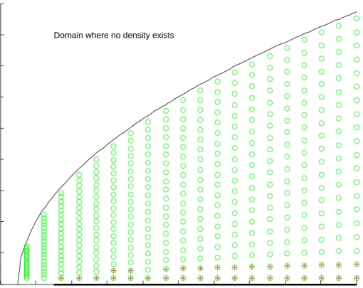
k, we considered a grid for skewness ranging from 0.1 to√k−1−0.1.For each point of this grid, say s, k, we computed α and β as described in Section 6.3 and recomputed the associated skewness and kurtosis, say ˜s,˜k.5 In Figure 1,
circles represent the points of the skewness-kurtosis grid for which we evaluated the parameters and, + symbols represent those points for which the distance
D= (s−˜s)2+ (k−˜k)2 >10−5.
This figure demonstrates several interesting phenomena 1) Even though, based on theoretical grounds, no density can exist on the segment (s= 0, k≥3), it is still possible to obtain a density for parameters close to the excluded seg-ment. 2) Even for very large values of kurtosis (limited in the figure to 20), we obtain a large range of values of skewness for which a highly accurate den-sity may be obtained. We also constructed a similar graph where kurtosis was allowed to took values up to 150. We find that, even for a kurtosis of 150, the range of skewness, where D < 10−5, ranges from 2.5 to 12.1, still a very respectable domain.
Many of the difficulties encountered in earlier attempts at such calculations
disappear in our approach. The linear transform Y =a+bZ allows us to write
the exponential quartic in terms of exp(−z4). Then, by replacing exp(−z4) by well-behaved discrete weights (this leads to formula (6.7)), we integrate directly over the range (−∞,∞), thus obviating the use of the logistic map. Next, we
4All of the programming was performed in the MATLAB environment. We implemented
the code on both Mac OS X and Windows Vista machines. All of the simulations were performed on a PC with an Intel quadricore processor running four MATLAB clones in parallel. To increase the speed of the computations, we transcribed the central part of the programs into the C language and called it via a MEX interface.
only optimize over two parameters, rather than four. We also feed optimized
starting values for α and β into the optimizer. These starting values are the
α and β corresponding to those points in the domain represented in Figure 1
that are closest to some given values of skewness and kurtosis. The skewness and kurtosis, and their associatedα and β, are stored once and for all in some file that is read into memory as the program is initialized.
To further understand some of the difficulties encountered in earlier studies, we obtained the parameters λj, for j = 0,· · · ,4 for extremely skewed cases,
and evaluated the resulting densities at points far out in the tail (sayz = 50 for a centered and reduced density) and still found a small, yet significant prob-ability mass. The logistic map, which transforms (−∞,∞) into (−1,1) used in the earlier work, may therefore have ‘fudged’ the behavior of the density for relatively large values of skewness and kurtosis. We also note that earlier work required many integration points (each evaluation costs time) whereas using abscissas and weights that are made specifically for the exp(−z4)
weight-ing function reduces the number of points for which the integrand needs to be evaluated.6
As the numerical exercises that follow will demonstrate, the time necessary to compute the required α and β parameters is of an order that is suitable for applying the exponential quartic in many econometric problems. The
compu-tation of one set of α and β requires about 0.015 seconds, allowing for about
66 density constructions per second. It is clear that the method proposed here is not confined to econometrics and may prove useful in other fields as well.
Similarly to the protocol described above, in the context of the parameter estimations related to QGPML2, we verified the precision of the computation of
δi, for i= 0,· · · ,2 for givenδ3, δ4, yielding a density with mean 0 and variance
1.
7.2. A First Experiment.
The objective of this first experiment was to demonstrate that the PML4 estimation may provide estimates which are superior to either the PML2 or the GMM estimators in an unconditional setting. We first discuss the choice of a data generating process, and then we focus on the estimation techniques. A priori, many distributions could be used for this experiment (Student-t, distri-butions in the Pearson family, Gamma, etc.) Preliminary work made it clear
6 We presently do not incorporate a selection rule on the number of abscissas, N, which
that a distribution should be chosen from which draws could be obtained in a very rapid manner. For this reason we settled on the family of skewed Laplace distributions, denoted sLD. These distributions have been used to price op-tions in the context of extreme return realizaop-tions, for example, by Gourier-oux and Monfort (2006). This family of distributions has three parameters,
b0 >0, b1 >0,and c, and its pdf is defined by:
f(z;b0, b1, c) = ( b 0b1 b0+b1 exp [b0(z−c)], if z ≤c, b0b1 b0+b1 exp [−b1(z−c)], if z > c. (7.1) The mean, variance, skewness and kurtosis of this density are given by:
m1(c, b0, b1) = E[Y] =c+ 1 b1 − 1 b0 , (7.2) σ2(c, b0, b1) = V ar[Y] = 1 b2 0 + 1 b2 1 , (7.3) s(c, b0, b1) = 2 σ3 1 b3 1 − 1 b3 0 , (7.4) k(c, b0, b1) = 9 σ4 1 b4 1 + 1 b4 0 + 6 σ4b2 0b21 . (7.5)
Since this density may be viewed as describing a mixture of exponentials, we use the inverse c.d.f. technique to simulate random draws from it.
In this first experiment, we focus on the situation where c = 0. Indeed,
without an additional assumption on one of the parameters of the sLD, we would not be able, in the following, to obtain parameter estimates based on the PML2 principle.
We simulated 10,000 samples, each of a length of either T = 25,50 or 100
i.i.d. observations. The estimation techniques used were ML, PML2, PML4 and GMM. Let us describe the way in which we implemented these estimations.
For ML, we maximized for each sample, the log-likelihood obtained from (7.1): LM L= T X i=1 Logf(zi;b0, b1).
For PML2, we considered the objective function:
LP M L2 =−T Logσ(b0, b1)− 1 2 T X i=1 zi−m1(b0, b1) σ(b0, b1) 2 .
For PML4, we formed the objective function:
LP M L4 =
T
X
i=1
where the parametersλ0,· · · , λ4 were computed as described in section 6.2 for
(m1(b0, b1), σ(b0, b1)2, s(b0, b1), k(b0, b1)).
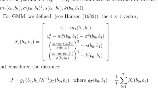
For GMM, we defined, (see Hansen (1982)), the 4×1 vector,
Xi(b0, b1) = zi−m1(b0, b1) zi2−m21(b0, b1)−σ2(b0, b1) zi−m1(b0,b1) σ(b0,b1) 3 −s(b0, b1) zi−m1(b0,b1) σ(b0,b1) 4 −k(b0, b1) ,
and considered the distance:
J =gT(b0, b1)0S−1gT(b0, b1), where gT(b0, b1) = 1 T T X i=1 Xi(b0, b1).
The GMM estimates were obtained as those parameters minimizing the distance
J. The matrix S that appears in the distance was obtained by using, as a
first step, the identity matrix, and as a second step, the asymptotic variance-covariance matrix. Thus, the GMM estimates are asymptotically optimal.
We performed the simulation using (b0, b1) = (2.41,1.30).7 This point
corre-sponds to the moments (m1, m2, s, k) = (1.30,0.35,1.15,6.91).
Table 1displays several statistics for 10,000 simulations and for various sam-ple sizes. However, the main result that this Table conveys is that, for all samsam-ple sizes considered, the MSE of the ML estimation dominates, as expected, over all other methods. However, we find that the PML4 technique yields estimates with an MSE up to less than half of the one for PML2. Concerning GMM, the parameters often hit the boundaries that we imposed during the estimation. The MSE of the parameters obtained by this method is the largest. This sug-gests that for situations where the econometrician has no prior information on the skewed distribution to use for the estimation, the PML4 technique may be a most useful one.
7.3. A Second Experiment.
In this experiment, we illustrate the robustness of the PML4 method with respect to the shape of the distribution as compared to that of the ML method. In order to be fair with the ML, we consider a situation in which the family of pdfs used to build the likelihood is allowed to reach the true moments up to fourth order, although it does not contain the true pdf. More precisely, the misspecified likelihood will be based on the family of skewed Laplace distribu-tions (sLD), and the true pdf will be that of a mixture of two normals whose
moments, up to the fourth order, are reachable by the sLD family. The skewed Laplace density family defined in (7.2) is conveniently reparametrized by the mean, µ, the standard error, σ, and a parameter, θ ∈ [0, π/2], such that the standardized variable (z −µ)/σ follows the zero-mean, unit-variance skewed Laplace density corresponding to b0 = 1/sinθ, b1 = 1/cosθ, c = sinθ−cosθ.
The pairs (s, k) that are reachable by the skewed Laplace density family are given by (7.4) and (7.5), where b0, b1 are replaced respectively by 1/sinθ and
1/cosθ, respectively, and σ is replaced by 1. Thus, the misspecified likelihood function is, T Y i=1 1 σf zi−µ σ ; 1 sinθ, 1
cosθ,sinθ−cosθ
, (7.6)
where f is given in (7.1).
The PML4 objective function is obtained by specifying the mean, variance, skewness, and kurtosis asµ, σ2,2(cos3θ−sin3θ)/(σ3),and 9(cos4θ+sin4θ)/(σ4)+
6 cos2θsin2θ/(σ4), respectively.
The data generating processes are mixtures of two normals such that µ =
0, σ2 = 1, with the skewness and kurtosis being obtained from the previous
formulae with θ = 10 (in degrees), namely s = 1.90 and k = 8.65. The family of two normals can reach any set of mean, variance, skewness, kurtosis, and this, moreover, can be reached in a non-unique way. Here, we choose two
data generating processes.8 First, we consider the unique mixture satisfying
µ= 0, σ2 = 1, s= 1.90, andk = 8.65 with the same variance in the two normal components. We find the mixture,
0.0451N(3.483,0.654) + (1−0.0451)N(−0.164,0.654),
where 0.654 is the standard deviation. Second, we choose the mixture maxi-mizing the entropy under the four constraints on the moments and find
0.102N(2.036,1.426) + (1−0.102)N(−0.232,0.597).
For these two DGPs, we use 10,000 simulations of T = 100 observations. For
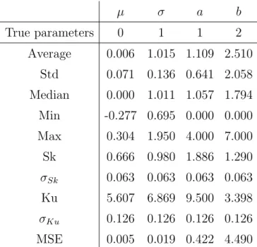
each simulation, we compute the misspecified ML estimates and the PML4 estimates of µ, σ, θ, where the true values are (0,1,10).
Table 2 displays the results from this simulation. Inspection of this Table reveals, for both DGPs, qualitatively similar results for the estimates of the parameters and the MSE. We find rather good estimates of both the mean and
8 More details on the construction of these processes are available upon request. The
the variance. The MSE of ˆσ tends to be better for the PML4 estimation than for the ML one.9 The deterioration of the estimate of the parameter θ, which commands higher moments is, however, dramatic if one uses a misspecified
model. For instance, focusing on the ML estimation, whereas the MSE of ˆµ is
0.0004, it becomes 327.49 for ˆθ.Inspecting of the average estimate of ˆθand its 5-and 95-percentiles reveals that the estimate is nearly three times the estimate of its true value. The 10% confidence intervals do not even contain the true value. On the other hand, if one considers the PML4 estimations, the deterioration of
the MSE of ˆθ is much less with an MSE=30.08. Also, the confidence intervals
now contain the true value.
As this experiment suggests, in the case of skewed and kurtic data, great care needs to be exercised if one uses ML estimation with a risk of misspecification. The PML4 method appears to be much more robust.
7.4. A Third Experiment.
In the previous examples, we demonstrated the usefulness of the PML4 tech-nique in an unconditional setting. In this section, we illustrate the usefulness of the PML4 technique in a conditional setting where the numerical complexity is much greater. There are situations where the modeling of the variation in higher
moments may be of importance per se. For instance, Hansen (1994) considered
a model in the spirit of Garch with time varying skewness and kurtosis. A generic model that captures variation in the higher moments is given by:
yi = µ+σεi,
whereεi ∼ D(0,1, s(xi), k∗(xi)),
s(xi) = 0.5 +axi, (7.7)
k∗(xi) = 2 +bxi, b >0,
xi ∼ U[1/2,3/2], i.i.d.
In the second line, D stands for some distribution where skewness and
over-kurtosis depends on some exogenous variable, xi. The next two lines specify
how skewness and over-kurtosis are parametrized. We recall that the kurtosis,
k, is related to the over-kurtosis, k∗, by k = 1 +s2 +k∗. For the simulations,
we take the lower moments to be µ = 0 and σ = 1. Furthermore, we take
a = 1 and b = 2. As long as the condition b > 0 is imposed in the numerical computation, the model will be well defined. The intercepts 0.5 and 2 in the
9This result is not due to statistical variation as we could verify by running the simulation
specification of s(xi) andk∗(xi) guarantee that the distribution will be skewed
(here s >1) and fat-tailed (here k >4).
TheDdistribution that we choose is the mixture of two normal distributions with identical variances as discussed in the previous subsection. In the
Monte-Carlo exercise, we simulate 1,500 samples, each with T = 100 observations.
The estimations require between about 60 and 340 sec, with an average time of about 130 sec.
Table 3 contains the statistics associated with the various estimations. As this Table demonstrates, even though the numerical complexity behind the PML4 computation is significant, this method may be actually implemented even in a Monte Carlo framework with many replications (here 1,500). With the feasibility of the method already demonstrated, we may now turn to the interpretation of the statistics. We first note that the parameters tend to be estimated rather well if one uses the average of the estimates. We find that the parameter estimates are skewed and kurtic, and we note that the MSE of the parameter estimates increases with the order of the moment that a given
parameter describes. The MSE of the mean µis 0.04. The MSE of the
param-eter b that describes the kurtosis of the distribution takes a much higher value of 4.490. We observe that parameters describing higher moments have higher associated MSE.
We conclude this section by noticing that our method may obviously be used in real applications, for models which may have more parameters, since it then has to be estimated only once.
7.5. A Fourth Experiment: QGPML2.
To validate the QGPML2 approach, we consider as DGP the observation (yi, xi) generated by: yi =axi+ exp(bxi)εi, ui ∼U(0,1), i.i.d. xi = (1 + 29ui)/10, θi = (1 + 29ui) π 180, εi ∼sLD 1 sinθi , 1 cosθi ,sinθi−cosθi . (7.8)
The first line specifies the mean and the variance of the model as depending on some exogenous variable xi. The second line defines the ui as uniform draws.
random numbersU(1/10,3). The fourth line specifiesθi as an angle that varies
between 1 and 30 degrees. The ratioπ/180 converts this angle into radians. The last equation specifies that εi is distributed according to the skewed Laplace
distribution with mean 0, variance 1, and known skewness and kurtosis. A similar parametrization was chosen in Subsection 7.3. We select as parameters
a= 1 and b= 1.
A preliminary simulation revealed that, for this parametrization, the skew-ness (kurtosis) of the εi ranges between 0 and 2 (respectively, 6 and 9).
The QGPML2 estimation is based on the following steps:
(1) Estimate a and b via PML2. This is tantamount to obtaining a, b by
maximizing the function:
T X i=1 −bxi− 1 2 yi−axi exp(bxi) 2 .
(2) Compute the first step estimators ˜λj,i for j = 1,· · · ,4 by using the
information contained ins(xi) andk(xi). This computation is described
in section 5.3. Notice that only ˜λ3i and ˜λ4i are used in the next step.
(3) Maximize, with respect to a and b, the objective function:
T X i=1 λ∗0,i+λ∗1,iyi+λ∗2,iy 2 i,
where,λ∗j,i =λ(axi,exp(bxi),˜λ3i,λ˜4i).The computation of the λ∗i,j may
be found in section 6.4. The resultingaandbestimates are the QGPML2 estimates.
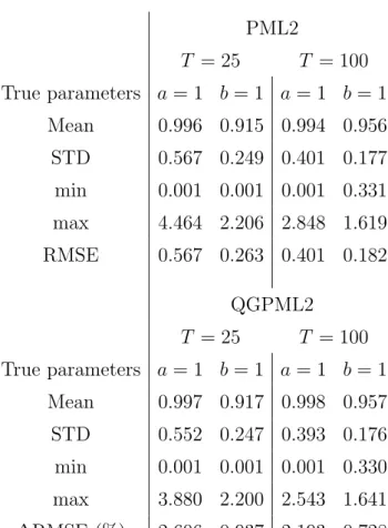
Table 4 reports some statistics for the simulations. Each time we use N = 30,000, a rather large number of simulations to ascertain that the findings are not spurious. We consider samples of size T = 25 and T = 100.10
Inspecting the table reveals that, as expected, the dispersion of the estimates obtained in the larger sample tends to be better. Comparing the dispersion of the parameters between the PML2 estimates and the QGPML2 estimates
reveals an improvement when using QGPML2.11 For instance, for T = 25,the
improvement of the RMSE of the parameter intervening in the mean,a, is 2.6%.
10Here, we focus on a large number of simulations each involving a relatively small sample.
The time required for this simulation could alternatively be devoted to the estimation of a model with either a larger sample or a more complex model structure involving several parameters.
11We did not pursue a search for settings where the efficiency gain may be more important,
as we simply wished to demonstrate the feasibility of the method here. We leave this pursuit for future research.
8. Conclusion
In this paper, we generalize the PML2 and QGPML1 methods proposed in Gourieroux, Monfort, and Trognon (1984). The main objective of these meth-ods was to propose consistent and asymptotically normal estimators of the pa-rameters which appear in the specification of the first two conditional moments, based on the optimization of possibly misspecified likelihood functions.
Here, we extend this approach by considering the first four conditional mo-ments. A key tool is the quartic exponential family. This family allows us to introduce PML4 and QGPML2 estimators, respectively, generalizing PML2 and QGPML1. A complete asymptotic theory is proposed. In particular, it is shown that the QGPML2 estimator reaches the semi-parametric bound based on the first two moments.
Another key issue is the numerical computation of the exponential quartic density parameters for given values of the first four moments. The solution adapted in this paper, which is based on an approach proposed by G. Freud (1986), appears to be very quick and stable, and it solves technical problems, which had been stressed in different strands of the literature, e.g. Maasoumi (1993), Ormoneit and White (1999).
In numerical studies, we not only demonstrate the feasibility of the proposed estimation methods, but also show that PML4 may provide more efficient esti-mates, in particular for small samples where GMM based estimates may have encountered difficulties. We also consider an example where an econometrician uses either a misspecified ML model or the PML4 model. In that case, the PML4 model demonstrates superior results. Lastly, we show the feasibility of the QGPML2 estimation, and in that context, we again prove gains in efficiency. Our estimation method may prove useful in many econometric applications that involve non-Gaussianity of some random variable. Beyond this, the pro-posed numerical techniques may be of relevance in Bayesian analysis, inde-pendent component analysis, and possibly physics, i.e. in situations where non-Gaussian distributions may be of relevance.
Appendix A. Properties of the Exponential Families
Let us consider the exponential family `(y, λ) = exp [λ0T(y)−ψ(λ)] defined in Section 2.1. An important issue is to characterize the range of the mapping
λ → Eλ[T(y)], for λ ∈ ˚Λ. Let us denote this mapping by ξ, and we denote
M =ξ(˚Λ), and C the closed convex hull of the support of νT.
We recall below a necessary and sufficient condition for whichM = ˚C due to Barndorff-Nielsen (1978). To this end, we need to recall the definition of asteep function [or alternatively an essentially smooth convex function (Rockafellar 1970)]. Introduce the following definition. Let ϕ:Rk →(−∞,∞) be a proper
convex function and D= {x∈ Rk : ϕ(x) <∞}. Assume that ˚D is not empty
and ϕ is differentiable throughout ˚D. Such a function will be defined to be
steep atx,where x∈DrD,˚ if limi→∞ | ∂x∂ϕ(xi)|=∞ whenever x1, x2, . . . , is a
sequence of points in ˚D converging tox. Furthermore, ϕ will be calledsteep if it is steep at all x∈DrD˚.
An exponential family is called steep if its cumulant generating function, ψ, is steep. It follows from this definition that a natural exponential family is called steep if limi→∞ | Eλi(T) |= +∞ whenever λ1, λ2, . . . , is a sequence of
points in ˚Λ converging to a point λ ∈Λr˚Λ.
A result due to Brown (1986, p. 72) provides a convenient, necessary, and sufficient condition for steepness. According to this result, the exponential family is steep if and only ifEλ(kT k) = ∞for allλ ∈Λr˚Λ.Unfortunately, this
condition is not satisfied by the exponential quartic family sinceT is integrable
in the Gaussian case, corresponding to values of λ satisfying λ4 = λ3 = 0,
λ2 <0,and which are in Λr˚Λ.
Appendix B. Computation of J(θ0) and I(θ0)
J(θ0) =− ∂2ϕ ∞(θ, P0) ∂θ∂θ0 =−EX " ∂2λ0(X, θ0) ∂θ∂θ0 + 4 X j=1 ∂2λj(X, θ0) ∂θ∂θ0 mj0 # ,
We have (omitting the variables X and θ0):
∂λj ∂θ = ∂m0 ∂θ ∂λj ∂m, j = 0, . . . ,4, ∂2λ j ∂θ∂θ0 = ∂m0 ∂θ ∂2λ j ∂m∂m0 ∂m ∂θ0 + 4 X k=1 ∂λj ∂mk ∂2m k ∂θ∂θ0,
J(θ0) =−EX ( ∂m0 ∂θ " ∂2λ 0 ∂m∂m0 + 4 X j=1 ∂2λ j ∂m∂m0mj0 # ∂m ∂θ0 ) − ( 4 X k=1 ∂λ0 ∂mk + ∂λ1 ∂mk m10+· · ·+ ∂λ4 ∂mk m40 ∂2mk ∂θ∂θ0 ) ,
and using Proposition 1, Corollary 1, and Proposition 2:
J(θ0) =EX ∂m0 ∂θ ∂λ0 ∂m ∂m ∂θ0 =EX ∂m0 ∂θ Σ −1∂m ∂θ0 . Similarly, I(θ0) =EXE0 ∂ϕ(Y, X, θ0) ∂θ ∂ϕ(Y, X, θ0) ∂θ0 =EXE0 ∂λ0 ∂θ + ∂λ0 ∂θT ∂λ0 ∂θ0 +T 0∂λ ∂θ0 , where ϕ(Y, X, θ) =P4 j=0λj(X, θ)Y j, and T0 = (Y, Y2, Y3, Y4).
Using Proposition 1, we have (omitting the variables X and θ0):
I(θ0) =EXE0 ∂λ0 ∂θ (T −m) (T −m) 0 ∂λ ∂θ0 =EX ∂λ0 ∂θ Ω ∂λ ∂θ0 =EX ∂m0 ∂θ ∂λ0 ∂mΩ ∂λ ∂m0 ∂m ∂θ0 =EX ∂m0 ∂θ Σ −1ΩΣ−1∂m ∂θ0 .
Appendix C. Asymptotic Behavior of the QGPML2
C.1. Preliminaries.
Let us consider the quartic family parametrized by ξ0 = (m1, σ2, λ3, λ4). If
we fix λ3, λ4 to a given value of λ∗3, λ
∗
4, then we obtain a family, indexed by
(m1, σ2), with log-density: 2 X j=0 λ∗j(ξ12)yj+λ∗3y 3+λ∗ 4y 4,
whereξ12 = (m1, σ2)0andλ∗j(ξ12) is a notation which stands forλ∗j(m1, σ2, λ∗3, λ
∗
4).
Differentiating with respect toξ12, we get 2 X j=0 ∂λ∗j ∂ξ12 mj = 0, (with m0 = 1) (C.1) and 2 X j=0 ∂2λ∗ j ∂ξ12∂ξ012 mj + ∂λ∗0 ∂ξ12 ∂m12 ∂ξ120 = 0, (C.2) with λ∗ = (λ∗1, λ∗2)0 and m12= (m1, m2)0. Moreover, ∂m12 ∂ξ0 12 = 1 0 2m1 1 ! . (C.3)
The variance-covariance matrix Σ1 of (Y, Y2)0 in this family is found easily.
For instance, we note that the pdf with respect to the measure µ∗ defined by
dµ∗(y) = exp(λ∗3y3 +λ∗
4y4)dy is exp [λ
∗
0(ξ12) +λ∗1(ξ12)y+λ∗2(ξ12)y2]. Using the
parametrization (λ∗1, λ∗2) and the general property of the exponential family given in 2.1 (2):
Σ1 =
∂m12
∂λ∗0 ,
which, written as a function ofξ12, leads to:
Σ1 = ∂m12 ∂ξ012 ∂ξ12 ∂λ∗0. We therefore have: ∂ξ12 ∂λ∗0 = ∂m12 ∂ξ120 −1 Σ1, hence: ∂λ∗ ∂ξ120 = Σ −1 1 ∂m12 ∂ξ120 . (C.4) C.2. Computation of J˜(θ0).
In the estimation based on the unfeasible equivalent estimator of the QGPML2, we have, noting θ12= (θ1, θ2) : ˜ J(θ0) =−EX ( 2 X j=0 ∂2λ∗ j ∂θ12∂θ012 m1(X, θ10), σ2(X, θ20), λ3(X, θ0), λ4(X, θ0)]mj(X, θ0)}.