Characterization of limacon gas expanders with consideration to the dynamics of apex seals and inlet control valve

COPYRIGHT NOTICE

FedUni ResearchOnline

https://researchonline.federation.edu.a

u

This is the submitted for peer-review version of the following article:

Phung, T. H. and I. A. Sultan (2018). "Characterization of limacon gas expanders with consideration to the dynamics of apex seals and inlet control valve." Journal of Engineering for Gas Turbines and Power 140(12).

Which has been published in final form at: https://doi.org/10.1115/1.4040418

© 2018 ASME.

This is the author’s version of the work. It is posted here with permission of the publisher for your personal use. No further distribution is permitted.

Characterisation of Limacon gas expanders with consideration to the dynamics of

apex seals and inlet control valve

Truong H. Phung, Ibrahim A. Sultan

[email protected], [email protected]

School of Engineering, Faculty of Science and Technology Federation University Australia

University Drive, Mount Helen, Victoria 3350, Australia

Abstract

Limaçon machine, of which the relative motion between the rotor and housing follows the limaçon curve, belongs to a class of rotary positive displacement machines. The profiles of rotors and housings of those machines can be constructed of either limaçon or circular curves, hence the names: limaçon-to-limaçon, circolimaçon, and limaçon-to-circular machines. This paper presents the investigation into the thermodynamic performance of the limaçon-to-circular machines with the presence of apex seals and inlet valve.

This paper sets out by briefly introducing the limaçon technology and the construction of the limaçon-to-circular machine working volume. The mathematical descriptions of ports’ positions and areas have also been introduced. The paper then discusses the flow and phase composition of working fluid through the working chambers as well as how the fluid velocity is modelled and calculated. Then the seal dynamic model and response of inlet valve are presented followed by the machine thermodynamic model. A case study has also been presented to show the responses of seals and inlet valve during the machine operation.

Keywords: Rotary machine; limaçon-to-circular; limaçon machine; limaçon motion; pump; gas expander;

compressor; positive displacement; optimisation; thermodynamics.

Article type: Research paper

Introduction

Over the past years, the consumption of fossil fuel continues to grow (International Energy Agency, 2015; Department of Industry and Science, 2015) due to the increase in energy demand in both heat and electricity forms. The growth in non-renewable resource consumption together with the low efficiency of the current energy conversion

processes result in enormous amount of excess heat is wasted and more greenhouse gas makes its way to the atmosphere. The energy generating activities are definitely key factors that drive the changes in our climate system and escalating risk for different aspect of life (IPCC, 2015; Climate Council, 2015).

From both the environmental and the technological point of view, it is essential to reduce the consumption of non-renewable resources by increasing the efficiency of energy conversion processes as a short-term strategy. The process efficiency can be increased by mean of heat recuperation – a practice that captures the previously overlooked waste heat to produce extra mechanical or electrical power. Organic Rankine Cycle (ORC) based micro power plants that utilise organic fluids to transfer heat and expand in the expander to give off work are often employed (Mathias, Johnston, Cao, Priedeman, & Christensen, 2009). Due to the relatively low temperature of low-grade heat, components of ORC micro power plants are often exposed to multi-phase flow; such a condition allows fluid droplets to be formed, which is not suitable for turbine technology. Lemort et al. (2009) and Sultan and Schaller (2011; 2012) in their published work have pointed out that the perfect candidates for low working fluid temperature, multi-phase flow, and low flow rate conditions are positive displacement machines, which include different embodiments of limaçon machines.

This paper investigates the output power and the efficiency of the limaçon-to-circular machine. A mathematical model has been developed based on the thermodynamic performance, seal dynamic, and inlet valve dynamic of such a machine. A case studies has been presented to test the reliability of such a model.

The limaçon-to-circular machine’s working volume

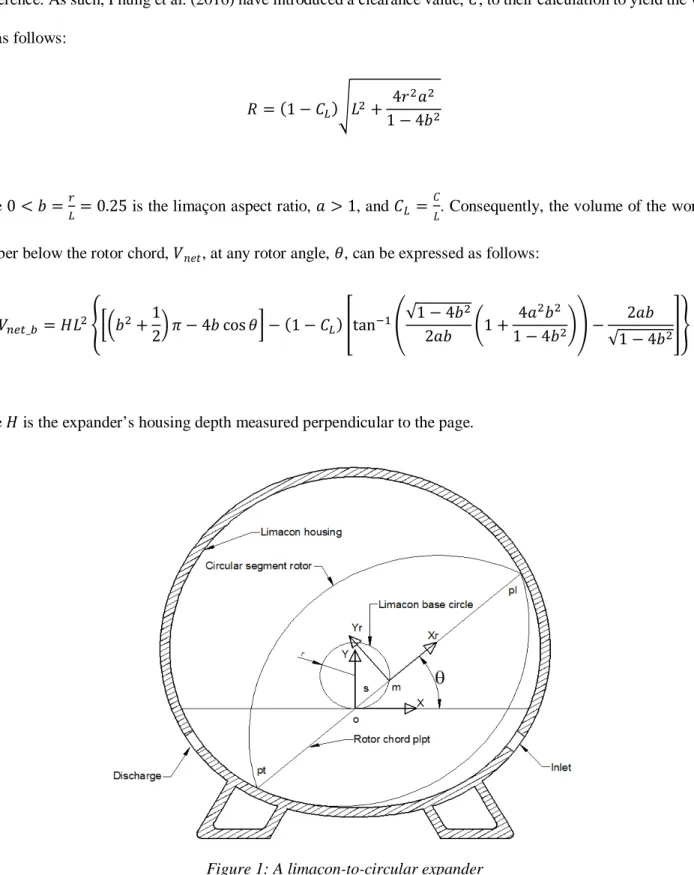
Detailed in Figure 1 is a limaçon-to-circular machine and its geometrical aspects. As shown in the figure, the limaçon chord, 𝑝𝑝_𝑙𝑙𝑝𝑝_𝑡𝑡, whose length is 2𝐿𝐿 is allowed to rotate and slide about the limaçon pole, 𝑜𝑜, which is the origin of a stationary frame 𝑋𝑋𝑋𝑋. The profile of the limaçon housing is formed by the trace of the apices, 𝑝𝑝_𝑙𝑙 or 𝑝𝑝_𝑡𝑡. Additionally, another frame namely 𝑋𝑋_𝑟𝑟𝑋𝑋_𝑟𝑟 is firmly attached to the rotor chord at its centre point, 𝑚𝑚, and moves with the chord. The angle 𝜃𝜃 measured from 𝑋𝑋-axis to 𝑋𝑋_𝑟𝑟-axis followed the right-hand sense is the angular displacement of the machine rotor. When the rotor is in motion, its centre point, m, stays kinematically attached to the base circle of radius, 𝑟𝑟. It is worth noticing that, the two lobes of such a limaçon-to-circular machine is constructed of two circular segments of radius, 𝑅𝑅, which take the chord, 𝑝𝑝_𝑙𝑙𝑝𝑝_𝑡𝑡, as the mirror line; hence, the machine received the name limaçon-to-circular machine. Phung, Sultan, and Boretti (2016) have pointed out that the housing and rotor of such a machine have distinct profiles (i.e.: limaçon housing, circular segment rotor) and the rotation of the rotor inside the

housing follows the limaçon housing; therefore, during operations this machine may encounter rotor-housing interference. As such, Phung et al. (2016) have introduced a clearance value, 𝐶𝐶, to their calculation to yield the value of 𝑅𝑅 as follows: 𝑅𝑅= (1− 𝐶𝐶𝐿𝐿)�𝐿𝐿2+ 4𝑟𝑟 2_𝑎𝑎2 1−4𝑏𝑏2 [1] where 0 <𝑏𝑏=𝑟𝑟

𝐿𝐿 = 0.25 is the limaçon aspect ratio, 𝑎𝑎 > 1, and 𝐶𝐶𝐿𝐿 = 𝐶𝐶

𝐿𝐿. Consequently, the volume of the working

chamber below the rotor chord, 𝑉𝑉_{𝑛𝑛𝑛𝑛𝑡𝑡}, at any rotor angle, 𝜃𝜃, can be expressed as follows:

𝑉𝑉𝑛𝑛𝑛𝑛𝑛𝑛_𝑏𝑏 =𝐻𝐻𝐿𝐿2���𝑏𝑏2+1₂� 𝜋𝜋 −4𝑏𝑏cos𝜃𝜃� −(1− 𝐶𝐶𝐿𝐿)�tan−1�√1−4𝑏𝑏 2 2𝑎𝑎𝑏𝑏 �1 + 4𝑎𝑎2_𝑏𝑏2 1−4𝑏𝑏2�� − 2𝑎𝑎𝑏𝑏 √1−4𝑏𝑏2�� [2] where 𝐻𝐻 is the expander’s housing depth measured perpendicular to the page.

Section 3 below introduces a model to calculate the instantaneous port area of the limaçon-to-circular machine as seen from the working chamber.

Inlet and outlet ports’ cross-sectional areas calculation

Sultan and Schaller (2011) have developed a concept to calculate the cross-sectional areas of the inlet and outlet ports of the limaçon-to-limaçon machine. The proposed concept treats both ports without discrimination; hence, no specific reference has been made to either port. As such, this paper will employ the similar approach to calculate the port areas for the limaçon-to-circular machine.

The radial positions of the port leading and trailing edges are defined by the two position vectors, 𝑹𝑹_𝑙𝑙 and 𝑹𝑹_𝑡𝑡, which are described in Figure 2. The leading edge is defined as the one that the rotor chord leading apex, 𝑝𝑝_𝑙𝑙, meets first during one cycle of operation. Those port edges vectors 𝑹𝑹_𝑙𝑙 and 𝑹𝑹_𝑡𝑡, can be expressed as follows:

�

𝑹𝑹𝑙𝑙 =𝐿𝐿

(

2𝑏𝑏sin𝜃𝜃𝑙𝑙+ 1

)

𝑹𝑹

�

𝑙𝑙 𝑹𝑹𝑡𝑡= 𝐿𝐿

(

2𝑏𝑏sin𝜃𝜃𝑡𝑡+ 1

)

𝑹𝑹

�

𝑡𝑡

[3]

where 𝜃𝜃_𝑙𝑙 is the leading edge, 𝜃𝜃_𝑛𝑛

is the trailing edge,

𝑹𝑹

�

_𝑙𝑙 =

�

cos𝜃𝜃𝑙𝑙 sin𝜃𝜃𝑙𝑙 0

�

and 𝑹𝑹

�

_𝑡𝑡=

�

cos𝜃𝜃𝑡𝑡 sin𝜃𝜃𝑡𝑡 0

�

are the unit vectors.

The angular location of the leading edge, 𝜃𝜃_𝑙𝑙< 𝜋𝜋

2, is defined first, followed by the port angular width, 𝛥𝛥𝜃𝜃𝑝𝑝. Hence, the angular position of the trailing edges can be calculated as: 𝜃𝜃_𝑡𝑡=𝜃𝜃_𝑙𝑙+𝛥𝛥𝜃𝜃_𝑝𝑝. The port length, 𝐿𝐿_𝑝𝑝, is given within the condition bounded by the rotor depth, 𝐻𝐻, in which 𝐿𝐿_𝑝𝑝< 𝐻𝐻. The port width, 𝑊𝑊, is calculated from the two edges vectors, 𝑹𝑹_𝑙𝑙 and 𝑹𝑹_𝑡𝑡, as:

𝑊𝑊= |𝑹𝑹𝑙𝑙− 𝑹𝑹𝑛𝑛|

[4] In this paper, the authors have utilised the semicircular shape for the port ends as described in Figure 2; hence, the full cross-sectional area of the port, 𝐴𝐴_𝑓𝑓, can be calculated as follows:

𝐴𝐴𝑓𝑓 =𝐿𝐿𝑝𝑝𝑊𝑊 − 𝑊𝑊2

�

1−𝜋𝜋₄

�

[5] In order to study the rotor-port interaction, which is the relation between the leading apex of the rotor and the port edges, the position of the rotor leading and trailing edges are defined as follows:

�

𝑷𝑷𝑙𝑙=𝐿𝐿

(

2𝑏𝑏sin𝜃𝜃+ 1

)

𝑿𝑿

�

𝑟𝑟 𝑷𝑷𝑡𝑡 =𝐿𝐿

(

2𝑏𝑏sin𝜃𝜃 −1

)

𝑿𝑿

�

𝑟𝑟

[6]

where 𝑿𝑿

�

_𝑟𝑟=

�

cos𝜃𝜃

sin𝜃𝜃

0

�

is a unit vector along the rotor chord, which is shown in Figure 2. The relative locations of the

rotor leading apex with respect to the port edges can now be defined using the two scalar quantity, 𝑠𝑠_𝑙𝑙 and 𝑠𝑠_𝑡𝑡, as follows: �𝑠𝑠𝑙𝑙 =�𝑹𝑹�𝑙𝑙×𝑿𝑿�𝑟𝑟� ∙ �𝑿𝑿�𝑟𝑟×𝒀𝒀�𝑟𝑟� 𝑠𝑠𝑛𝑛 =�𝑹𝑹�𝑛𝑛×𝑿𝑿�𝑟𝑟� ∙ �𝑿𝑿�𝑟𝑟×𝒀𝒀�𝑟𝑟� [7] where 𝒀𝒀

�

_𝑟𝑟=

�

−sin𝜃𝜃 cos𝜃𝜃 0

�

is a unit vector along the axis perpendicular to the rotor chord (Figure 2).

The port areas can now be determined from one of the following four cases:

• Case 1: when 𝑠𝑠_𝑙𝑙 ≥0 and 𝑠𝑠_𝑡𝑡≥ 0, it is suggested that the port is fully open to the control volume. In this case the port instantaneous area, 𝐴𝐴_𝑝𝑝, can be set equal to the full area, 𝐴𝐴_𝑓𝑓.

• Case 2: when 𝑠𝑠_𝑙𝑙≥ 0 and 𝑠𝑠_𝑡𝑡 < 0, it is suggested that the port is being progressively opened to the control volume. In this case the port area, 𝐴𝐴_𝑝𝑝, can be approximated using the equation 𝐴𝐴_𝑝𝑝=𝐴𝐴_𝑓𝑓|𝑷𝑷𝑙𝑙−𝑹𝑹𝑙𝑙|

𝑊𝑊 .

• Case 3: when 𝑠𝑠_𝑙𝑙 < 0 and 𝑠𝑠_𝑡𝑡 ≥0, it is suggested that the port is being progressively shut off from the control volume. In this case the port area, 𝐴𝐴_𝑝𝑝, can be approximated using the equation 𝐴𝐴_𝑝𝑝 =𝐴𝐴_𝑓𝑓|𝑷𝑷𝑡𝑡−𝑹𝑹𝑡𝑡|

𝑊𝑊 . • Case 4: when 𝑠𝑠_𝑙𝑙> 0 and 𝑠𝑠_𝑡𝑡 < 0, it is suggested that the port is totally shut off from the control volume.

The above four cases of the port areas can be summarised as follows:

⎩

⎪

⎪

⎨

⎪

⎪

⎧

_{𝑖𝑖𝑓𝑓𝑠𝑠} 𝑙𝑙≥ 0 𝑎𝑎𝑛𝑛𝑎𝑎

�

𝑠𝑠𝑡𝑡≥ 0 𝑡𝑡ℎ𝑛𝑛𝑛𝑛𝐴𝐴𝑝𝑝= 𝐴𝐴𝑓𝑓 𝑠𝑠𝑡𝑡< 0 𝑡𝑡ℎ𝑛𝑛𝑛𝑛𝐴𝐴𝑝𝑝= 𝐴𝐴𝑓𝑓

|

𝑷𝑷𝑙𝑙− 𝑹𝑹𝑙𝑙

|

𝑊𝑊 𝑖𝑖𝑓𝑓𝑠𝑠_𝑙𝑙 < 0 𝑎𝑎𝑛𝑛𝑎𝑎

�

𝑠𝑠𝑡𝑡≥0 𝑡𝑡ℎ𝑛𝑛𝑛𝑛𝐴𝐴𝑝𝑝=𝐴𝐴𝑓𝑓

|

𝑷𝑷𝑡𝑡_𝑊𝑊− 𝑹𝑹𝑡𝑡

|

𝑠𝑠𝑡𝑡 < 0 𝑡𝑡ℎ𝑛𝑛𝑛𝑛𝐴𝐴𝑝𝑝 = 0 [8] The velocity of fluid flow through the port will be studied in section 4 below.

Fluid velocity through ports

The flow of the working fluid through the ports of the limaçon machine encounters a sudden expansion and a change in direction, this type of flow is similar to that of the globe valves; therefore, these limaçon-to-circular machines’ ports can be approximated as globe valves rather than orifices. McNeil (1999), who also referred to the work of Fairhurst (1983) on globe valves, has published work on the approximation of flow in orifice plates, gate valves as well as globe valves.

The flow through ports undergoes an energy conversion process, which can be described as an equation to calculate the velocity at the downstream side of the ports:

𝑈𝑈=�2(ℎ𝑢𝑢− ℎ𝑑𝑑) =√2𝛥𝛥ℎ

[9] Figure 2: The limaçon-to-circular port area

where ℎ_𝑢𝑢 and ℎ_𝑎𝑎 are the up-stream and down-stream isentropic enthalpy, respectively

𝛥𝛥ℎ is an isentropic enthalpy drop along the flow direction

When the losses due to friction and the change in cross-sectional area are taken into account, equation [9] can be re-written as a function of the enthalpy drop and the loss coefficient, 𝐾𝐾_𝑝𝑝= 𝑁𝑁_𝑝𝑝𝑓𝑓, as follows (Massoud, 2005):

𝑈𝑈 =�2_𝐾𝐾𝛥𝛥ℎ 𝑝𝑝

[10]

where 𝑁𝑁_𝑝𝑝 is a specific number given for a specific type of flow and 𝑓𝑓 is a friction factor for turbulent flow. The friction factor, 𝑓𝑓, can be calculated using the Colebrook correlation (Munson, Rothmayer, Okiishi, & Huebsch, 2013) as follows: 1

�

𝑓𝑓=−2.0𝑙𝑙𝑜𝑜𝑙𝑙

�

𝜀𝜀/𝐷𝐷 3.7 + 2.51 𝑅𝑅𝑛𝑛

�

𝑓𝑓

�

[11] where 𝜀𝜀 is the surface roughness, 𝐷𝐷 is the diameter or hydraulic diameter of the pipe or the flow container, and 𝑅𝑅𝑛𝑛 is the Reynolds number. Equation [11], however, requires iteration to solve for the friction factor, 𝑓𝑓. Hence, Massoud (2005) suggested that in most engineering applications where smooth pipes are utilised and the flow is fully developed turbulent, the friction factor can be expressed using the McAdams formulation:

𝑓𝑓=0.184_{𝑅𝑅𝑛𝑛0.2} = 0.184

�𝜌𝜌𝜌𝜌𝜌𝜌_𝜇𝜇 �0.2

[12]

From the definition of Reynolds number, 𝑅𝑅𝑛𝑛=𝜌𝜌𝜌𝜌𝜌𝜌

𝜇𝜇 , equations [10] and [12] can be utilised to find the velocity

of flow through the inlet port of the limaçon-to-circular machine as:

𝑈𝑈𝑖𝑖=

⎩

⎪

⎪

⎨

⎪

⎪

⎧

�

_0.1842𝛥𝛥ℎ_𝑁𝑁 𝑝𝑝

�

5 9

�

𝜌𝜌𝑖𝑖𝑎𝑎𝐷𝐷𝑖𝑖𝑎𝑎 𝜇𝜇_{𝑖𝑖𝑎𝑎}

�

1 9 𝑖𝑖𝑓𝑓

√

2𝛥𝛥ℎ <𝑈𝑈𝑠𝑠 𝑈𝑈_𝑠𝑠 11 10

�

0.184𝑁𝑁_𝑝𝑝

�

𝜌𝜌_{𝑖𝑖𝑎𝑎}𝐷𝐷𝑖𝑖𝑎𝑎 𝜇𝜇_{𝑖𝑖𝑎𝑎}

�

1 10 𝑖𝑖𝑓𝑓

√

2𝛥𝛥ℎ> 𝑈𝑈𝑠𝑠 [13]

where subscript 𝑖𝑖 represents the flow through the inlet port.

𝜌𝜌_{𝑖𝑖𝑎𝑎},𝐷𝐷𝑖𝑖𝑎𝑎,𝑎𝑎𝑛𝑛𝑎𝑎𝜇𝜇𝑖𝑖𝑎𝑎 are the down-stream density, hydraulic diameter, and viscosity, respectively. 𝑈𝑈𝑠𝑠 is the speed of sound on the down-stream side of the port

The above equation can also be used to calculate the velocity of flow through the outlet port by replacing the subscript 𝑖𝑖 for the inlet, by 𝑜𝑜 for the outlet. Equation [13] can be utilised for both single and two-phase flow situations. In two-phase flow condition, the homogeneous flow model (Fairhurst, 1983) is to be employed and used in line with equations [12] and [13], in which the equivalent viscosity is obtained using the McAdams’ equation as follows:

1 𝜇𝜇_{𝑖𝑖𝑎𝑎} = 𝑥𝑥 𝜇𝜇_{𝑣𝑣𝑎𝑎𝑝𝑝}+ 1− 𝑥𝑥 𝜇𝜇_{𝑙𝑙𝑖𝑖𝑎𝑎} [14]

where 𝜇𝜇_{𝑖𝑖𝑎𝑎} is the equivalent down-stream viscosity of the inlet port

𝜇𝜇_{𝑣𝑣𝑎𝑎𝑝𝑝}, and 𝜇𝜇_{𝑙𝑙𝑖𝑖𝑎𝑎} are the viscosities of the vapour and liquid phase, respectively

𝑥𝑥=𝑚𝑚𝑚𝑚𝑚𝑚𝑚𝑚𝑓𝑓𝑙𝑙𝑓𝑓𝑓𝑓𝑟𝑟𝑚𝑚𝑛𝑛𝑛𝑛_{𝑛𝑛𝑓𝑓𝑛𝑛𝑚𝑚𝑙𝑙𝑚𝑚𝑚𝑚𝑚𝑚𝑚𝑚}𝑓𝑓𝑓𝑓_{𝑓𝑓𝑙𝑙𝑓𝑓𝑓𝑓𝑟𝑟𝑚𝑚𝑛𝑛𝑛𝑛}𝑛𝑛ℎ𝑛𝑛𝑔𝑔𝑚𝑚𝑚𝑚𝑝𝑝ℎ𝑚𝑚𝑚𝑚𝑛𝑛=_𝑚𝑚̇ 𝑚𝑚̇𝑔𝑔𝑔𝑔𝑔𝑔

𝑙𝑙𝑙𝑙𝑙𝑙𝑙𝑙𝑙𝑙𝑙𝑙+𝑚𝑚̇𝑔𝑔𝑔𝑔𝑔𝑔 is the dryness fraction (Ryley, 1964)

Additionally, the speed of sound of the two-phase flow can be calculated either by using the available REFPROP functions offered by Lemmon et al. (2010) or based on the equilibrium of mechanical, thermal, and fluid phase assumptions, such an approach is detailed in the published work by Lund and Flatten (2010). The accuracy of the speed of sound can also be improved by using the two methods simultaneously.

With the utilisation of the loss coefficient, 𝐾𝐾_𝑝𝑝, and the McAdams formulation, the velocity of fluid flows through the inlet and outlet ports can be calculated using equation [13] in a non-iterative manner. Moreover, the employment of the enthalpy difference instead of pressure difference has excluded the need of calculating the expansion factor during the expansion process in two-phase flow condition. Hence, in the following section, the flow velocity equation [13] will be put in to use in accordance with the continuity and energy equations in order to obtain a thermodynamic model for the limaçon-to-circular machine.

The seal dynamic model

In order to reduce the leakages and improve the efficiency, the limaçon machine will require sealing for both the apex-housing and the side gaps. The side seals experience relatively constant pressure difference and no gap

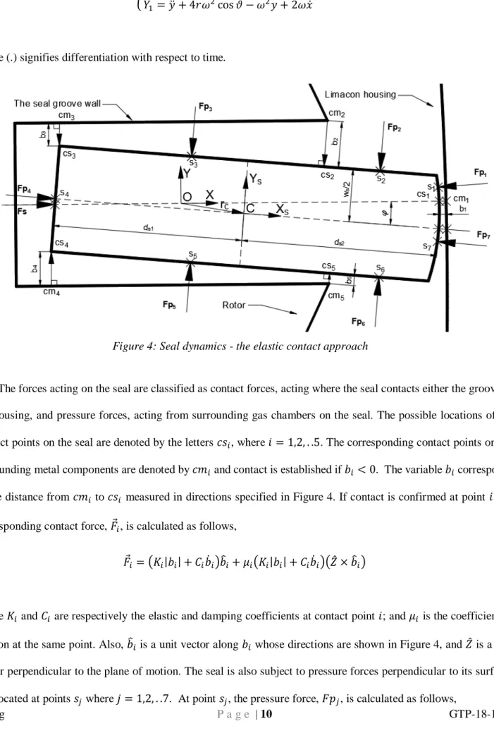
changes during machine operation. On the other hand, the apex-seals are subject to severe dynamic effects as they undergo alternating pressures from the machine chambers as well as changing distance from the seal apex to its corresponding point on the housing. This gives rise to the need to investigate the impact of the motion of the seal relative to the rotor, housing, and seal-groove on the machine performance and functioning. Even though the dynamic model of the apex seal is fairly complex and is a topic of a separate publication, an attempt is made here to summarise the seal dynamic model in such a manner which enables the reader to capture the fundamental aspects of this model. The seal axial length 𝑎𝑎_𝑚𝑚 can also be described as 𝑎𝑎_𝑚𝑚 =𝑎𝑎_𝑚𝑚1+𝑎𝑎_𝑚𝑚2 where 𝑎𝑎_𝑚𝑚1 and 𝑎𝑎_𝑚𝑚2 are measured form the seal centre of gravity (CG) to either end of the seal (Figure 4). Figure 3shows the position of the seal with respect to the rotor axis and the pole of the limaçon curve. The figure also shows the angle, 𝜆𝜆, between the rotor axis and the direction along which the housing reaction is directed as per the kinematical aspects of the limaçon design.

The position, 𝑟𝑟_𝑐𝑐1, of the seal CG with respect to the frame 𝑋𝑋₁𝑋𝑋₁ which is a situated at the pole and rotates with the rotor is given by,

𝑟𝑟𝑐𝑐1= (2𝑟𝑟sin𝜃𝜃+𝐿𝐿𝑖𝑖 +𝑥𝑥)𝚤𝚤̂+𝑦𝑦𝚥𝚥̂

[15] where 𝚤𝚤̂ and 𝚥𝚥̂ are unit vectors in the directions of 𝑋𝑋₁ and 𝑋𝑋₁ respectively. 𝐿𝐿_𝑖𝑖 in equation [15] is the distance from the rotor centre to the initial location of the seal CG. The symbols 𝑥𝑥 and 𝑦𝑦 signify small deflections of the seal CG in the

direction of the axes of the frame 𝑋𝑋₁𝑋𝑋₁. As the rotor rotates with a constant angular velocity, 𝜔𝜔, the accelerations of the seal CG in the direction of 𝑋𝑋₁ and 𝑋𝑋₁ respectively are given as follows,

�𝑋𝑋̈1=𝑥𝑥̈ −4𝑟𝑟𝜔𝜔2sin𝜗𝜗 − 𝜔𝜔2𝐿𝐿𝑖𝑖− 𝜔𝜔2𝑥𝑥 −2𝜔𝜔𝑦𝑦̇ 𝑋𝑋̈1=𝑦𝑦̈+ 4𝑟𝑟𝜔𝜔2cos𝜗𝜗 − 𝜔𝜔2𝑦𝑦+ 2𝜔𝜔𝑥𝑥̇

[16] where (.) signifies differentiation with respect to time.

The forces acting on the seal are classified as contact forces, acting where the seal contacts either the groove or the housing, and pressure forces, acting from surrounding gas chambers on the seal. The possible locations of the contact points on the seal are denoted by the letters 𝑐𝑐𝑠𝑠_𝑖𝑖, where 𝑖𝑖 = 1,2, . .5. The corresponding contact points on the surrounding metal components are denoted by 𝑐𝑐𝑚𝑚_𝑖𝑖 and contact is established if 𝑏𝑏_𝑖𝑖 < 0. The variable 𝑏𝑏_𝑖𝑖 corresponds to the distance from 𝑐𝑐𝑚𝑚_𝑖𝑖 to 𝑐𝑐𝑠𝑠_𝑖𝑖 measured in directions specified in Figure 4. If contact is confirmed at point 𝑖𝑖, the corresponding contact force, 𝐹𝐹⃗_𝑖𝑖, is calculated as follows,

𝐹𝐹⃗𝑖𝑖=�𝐾𝐾𝑖𝑖|𝑏𝑏𝑖𝑖| +𝐶𝐶𝑖𝑖𝑏𝑏̇𝑖𝑖�𝑏𝑏�𝑖𝑖+𝜇𝜇𝑖𝑖�𝐾𝐾𝑖𝑖|𝑏𝑏𝑖𝑖| +𝐶𝐶𝑖𝑖𝑏𝑏̇𝑖𝑖��𝑍𝑍̂×𝑏𝑏�𝑖𝑖�

[17] where 𝐾𝐾_𝑖𝑖 and 𝐶𝐶_𝑖𝑖 are respectively the elastic and damping coefficients at contact point 𝑖𝑖; and 𝜇𝜇_𝑖𝑖 is the coefficient of friction at the same point. Also, 𝑏𝑏�_𝑖𝑖 is a unit vector along 𝑏𝑏_𝑖𝑖 whose directions are shown in Figure 4, and 𝑍𝑍̂ is a unit vector perpendicular to the plane of motion. The seal is also subject to pressure forces perpendicular to its surfaces and located at points 𝑠𝑠_𝑗𝑗 where 𝑗𝑗= 1,2, . .7. At point 𝑠𝑠_𝑗𝑗, the pressure force, 𝐹𝐹𝑝𝑝_𝑗𝑗, is calculated as follows,

𝐹𝐹𝑝𝑝

�����⃗_{𝑗𝑗=𝐴𝐴𝑗𝑗𝑃𝑃𝑗𝑗𝑓𝑓̂𝑚𝑚𝑗𝑗}

[18]

where 𝐴𝐴_𝑗𝑗 is the seal surface area near point 𝑠𝑠_𝑗𝑗, 𝑃𝑃_𝑗𝑗 is the gas pressure near the same point and 𝑓𝑓̂_{𝑚𝑚𝑗𝑗} signifies a unit vector inwards perpendicular to the surface whose area is 𝐴𝐴_𝑗𝑗. The total forces, 𝐹𝐹⃗, acting on the seal is therefore calculated as follows, 𝐹𝐹⃗ =𝐹𝐹𝑥𝑥𝑋𝑋�1+𝐹𝐹𝑦𝑦𝑋𝑋�1 =𝐹𝐹⃗𝑚𝑚+� 𝐹𝐹⃗𝑖𝑖 5 𝑖𝑖=1 +� 𝐹𝐹𝑝𝑝�����⃗𝑗𝑗 7 𝑗𝑗=1 [19]

where 𝐹𝐹⃗_𝑚𝑚 is the sum of the elastic and damping forces acting on the back end of the seal where the supporting spring is fitted.

Once all the forces have been calculated, three nonlinear differential equations are written for the system in the following form: �𝑚𝑚0𝑚𝑚 𝑚𝑚0𝑚𝑚 00 0 0 𝐼𝐼𝐶𝐶𝐶𝐶 � �𝑋𝑋̈𝑋𝑋̈11 𝜑𝜑̈ �=� 𝐹𝐹𝑥𝑥 𝐹𝐹𝑦𝑦 ∑𝑀𝑀𝐶𝐶𝐶𝐶 � [20] where 𝑚𝑚_𝑚𝑚 is the mass of the seal and 𝐼𝐼_{𝐶𝐶𝐶𝐶} is the mass moment of inertia of the seal about is CG. Moreover, ∑ 𝑀𝑀_{𝐶𝐶𝐶𝐶} signifies the moment of various forces about the seal CG. In equation [20], 𝜑𝜑̈ is the angular acceleration of the seal and the two linear acceleration components, 𝑋𝑋̈₁ and 𝑋𝑋̈₁, have been introduced in equation [16].

The three differential equations in [20] are solved numerically at every rotor angle to find the corresponding linear and angular deflections of the seal at this rotor angle. Leakage past the seal-housing gap is confirmed if the distance 𝑏𝑏₁ is found to be positive. In this case the amount of leakage is calculated by employing the orifice model to calculate the flow past the seal.

Dynamic response of inlet valve

To control the amount of fluid entering the machine chamber to be expanded, a control valve is fitted at the inlet as shown in Figure 5. The inclusion of an inlet valve has subsequently created an antechamber, 𝑉𝑉₃, which separates the inlet passage and the machine working chambers. Hence, during the machine operation, fluid will need to fill this antechamber before entering the upper chamber instead of flowing directly from the inlet to the upper chamber as in

the case of no-inlet-valve design. Figure 5 shows that depends on the angular position of the rotor, then antechamber can expose itself to either the upper chamber, the lower chamber, or both at the same time. The inlet valve is of a normally open type and kept open by a spring, 𝑘𝑘_𝑣𝑣, as shown in Figure 5. The spring force, 𝑘𝑘_𝑣𝑣𝛿𝛿_𝑣𝑣, is large enough to keep the valve open even when the top surface of the valve is exposed to pressure from the supply tank. The valve stem is connected to a lever which is then connected to a plunger the motion of which controls the valve opening and closing. Movement of the plunger is controlled by two solenoids installed at the two ends of the stem (Figure 5). One solenoid helps closing the valve to cut off fluid supply, the other assists the spring during the valve opening phase. This design aims to reduce the valve response time and ensures that the machine can still functioning in case one or both of the solenoids fail. Of note is the position of the pivot point, this point is located closer to the valve stem than to the plunger; the distances from pivot point to the valve stem and plunger are 𝑎𝑎 and 𝑏𝑏, respectively. The ratio of the arms will help increasing the amount of force acting on the valve steam at the same time reducing the current load on the solenoid coils.

It is now essential to derive the equation of motion of this plunger-lever-valve system. The mass of the plunger, the lever, and the valve are defined as 𝑚𝑚₁,𝑚𝑚₂, and 𝑚𝑚₃ respectivety. The distances the valve and the plunger travel in vertical direction are 𝑧𝑧_𝑣𝑣 and 𝑥𝑥_𝑣𝑣, respectively; linear motion of the centre of gravity (CG) of the lever in the vertical direction is 𝑦𝑦_𝑣𝑣. The potential energy and kinetic energies of the system can be expressed as:

𝑃𝑃𝑃𝑃=1₂𝑘𝑘𝑣𝑣(𝛿𝛿𝑣𝑣+𝑥𝑥𝑣𝑣)2+𝑚𝑚1𝑙𝑙𝑥𝑥𝑣𝑣+𝑚𝑚2𝑙𝑙𝑦𝑦𝑣𝑣− 𝑚𝑚3𝑙𝑙𝑧𝑧𝑣𝑣

[21] and

𝐾𝐾𝑃𝑃=1₂𝑚𝑚1𝑥𝑥̇𝑣𝑣2+1₂𝑚𝑚2𝑦𝑦̇𝑣𝑣2+1₂𝑚𝑚3𝑧𝑧̇𝑣𝑣2+1₂𝐼𝐼2𝜃𝜃̇𝑣𝑣2

[22] Equation [21] and [22] can be rewritten in terms of 𝑧𝑧_𝑣𝑣 and 𝑧𝑧̇_𝑣𝑣 as follows:

𝑃𝑃𝑃𝑃=1₂𝑘𝑘𝑣𝑣�𝛿𝛿𝑣𝑣+𝑧𝑧𝑣𝑣𝑏𝑏_𝑎𝑎� 2 +�𝑚𝑚1𝑏𝑏_𝑎𝑎+𝑚𝑚2�𝑏𝑏 − 𝑎𝑎_{2𝑎𝑎 � − 𝑚𝑚}3� 𝑙𝑙𝑧𝑧𝑣𝑣 [23] and 𝐾𝐾𝑃𝑃=1₂𝑚𝑚1�𝑏𝑏_𝑎𝑎� 2 𝑧𝑧̇𝑣𝑣2+1₂𝑚𝑚2�𝑎𝑎₂+_{𝑎𝑎 �}𝑏𝑏 2 𝑧𝑧̇𝑣𝑣2+1₂𝑚𝑚3𝑧𝑧̇2+1_2𝑎𝑎𝐼𝐼2₂𝑧𝑧̇𝑣𝑣2 𝐾𝐾𝑃𝑃=1₂�𝑚𝑚1�𝑏𝑏_𝑎𝑎� 2 +𝑚𝑚2�𝑎𝑎₂+_{𝑎𝑎 �}𝑏𝑏 2 +𝑚𝑚3+_𝑎𝑎𝐼𝐼2₂� 𝑧𝑧̇𝑣𝑣2 [24] where 𝑘𝑘_𝑣𝑣 is the spring stiffness; 𝛿𝛿_𝑣𝑣 is the spring initial deflection. The spring is aligned with the solenoids plungers

𝐼𝐼2 is the moment of inertia of the lever about the pivot point 𝑥𝑥̇𝑣𝑣,𝑦𝑦̇𝑣𝑣, and 𝑧𝑧̇𝑣𝑣 are the velocity of 𝑚𝑚1,𝑚𝑚2, and 𝑚𝑚3, respectively.

Differentiating the equation of potential energy with respect to 𝑧𝑧_𝑣𝑣 and kinetic energy with respect to 𝑧𝑧̇_𝑣𝑣 give:

𝜕𝜕𝑃𝑃𝑃𝑃 𝜕𝜕𝑧𝑧𝑣𝑣 =𝑘𝑘𝑣𝑣 𝑏𝑏 𝑎𝑎 �𝛿𝛿𝑣𝑣+𝑧𝑧𝑣𝑣 𝑏𝑏 𝑎𝑎�+�𝑚𝑚1 𝑏𝑏 𝑎𝑎+𝑚𝑚2� 𝑏𝑏 − 𝑎𝑎 2𝑎𝑎 � − 𝑚𝑚3� 𝑙𝑙 [25] and 𝜕𝜕𝐾𝐾𝑃𝑃 𝜕𝜕𝑧𝑧̇𝑣𝑣 =�𝑚𝑚1� 𝑏𝑏 𝑎𝑎� 2 +𝑚𝑚2�𝑎𝑎₂+_{𝑎𝑎 �}𝑏𝑏 2 +𝑚𝑚3+_𝑎𝑎𝐼𝐼2₂� 𝑧𝑧̇𝑣𝑣 [26]

Based on the Lagrange energy method, the equation of motion of this system can be written as �𝑚𝑚1�𝑏𝑏_𝑎𝑎� 2 +𝑚𝑚2�𝑎𝑎₂+_{𝑎𝑎 �}𝑏𝑏 2 +𝑚𝑚3+_𝑎𝑎𝐼𝐼2₂� 𝑧𝑧̈𝑣𝑣+𝑐𝑐𝑛𝑛𝑒𝑒𝑧𝑧̇𝑣𝑣+𝑘𝑘𝑧𝑧𝑣𝑣�𝑏𝑏_𝑎𝑎� 2 =−𝑘𝑘𝑣𝑣𝛿𝛿𝑣𝑣�𝑏𝑏_{𝑎𝑎� −}�𝑚𝑚1𝑏𝑏_𝑎𝑎+𝑚𝑚2�𝑏𝑏 − 𝑎𝑎_{2𝑎𝑎 � − 𝑚𝑚}3� 𝑙𝑙+Δ𝑃𝑃𝐶𝐶𝑑𝑑𝐴𝐴𝑣𝑣+𝐹𝐹𝑚𝑚𝑙𝑙𝑏𝑏_𝑎𝑎+𝐹𝐹𝑚𝑚𝑢𝑢𝑟𝑟 [27] where 𝑐𝑐_{𝑛𝑛𝑒𝑒} is the equivalent damping coefficient;

Δ𝑃𝑃=𝑃𝑃𝑖𝑖𝑛𝑛− 𝑃𝑃3 is the difference in pressure between the inlet and antechamber; 𝐶𝐶𝑑𝑑 is the drag coefficient of the valve, 0.6≤ 𝐶𝐶𝑑𝑑 ≤0.9

𝐴𝐴𝑣𝑣 is the area of the vale that is subjected to the effect of pressure difference; 𝐹𝐹𝑚𝑚𝑙𝑙 is the force exerted by the solenoids; and

𝐹𝐹𝑚𝑚𝑢𝑢𝑟𝑟 is the contact force that the valve experiences either from the seat or from the mechanical stopper.

The force 𝐹𝐹_{𝑚𝑚𝑢𝑢𝑟𝑟} can be calculated by using the Algorithm 1 as follows:

Algorithm 1: Calculate the force 𝐹𝐹_{𝑚𝑚𝑢𝑢𝑟𝑟} 1 𝒊𝒊𝒊𝒊𝑧𝑧_𝑣𝑣>𝑠𝑠_{𝑚𝑚𝑛𝑛} 2 𝐹𝐹_{𝑚𝑚𝑢𝑢𝑟𝑟}=−𝑘𝑘_{𝑚𝑚𝑛𝑛𝑚𝑚𝑛𝑛}(𝑧𝑧_𝑣𝑣− 𝑠𝑠_{𝑚𝑚𝑛𝑛})− 𝑐𝑐_{𝑚𝑚𝑛𝑛𝑚𝑚𝑛𝑛}𝑧𝑧̇_𝑣𝑣 3 𝒆𝒆𝒆𝒆𝒆𝒆𝒆𝒆𝒊𝒊𝒊𝒊𝑧𝑧_𝑣𝑣 < 0 4 𝐹𝐹_{𝑚𝑚𝑢𝑢𝑟𝑟}=−𝑘𝑘_{𝑚𝑚𝑛𝑛𝑓𝑓𝑝𝑝}𝑧𝑧_𝑣𝑣− 𝑐𝑐_{𝑚𝑚𝑛𝑛𝑓𝑓𝑝𝑝}𝑧𝑧̇_𝑣𝑣 5 𝒆𝒆𝒆𝒆𝒆𝒆𝒆𝒆 6 𝐹𝐹_{𝑚𝑚𝑢𝑢𝑟𝑟}= 0 7 𝒆𝒆𝒆𝒆𝒆𝒆

where 𝑠𝑠_{𝑚𝑚𝑛𝑛} is the stroke or the maximum motion of the valve stem

𝑘𝑘𝑚𝑚𝑛𝑛𝑚𝑚𝑛𝑛 and 𝑘𝑘𝑚𝑚𝑛𝑛𝑓𝑓𝑝𝑝 are the stiffness of the seat and mechanical stopper, respectively

𝑐𝑐𝑚𝑚𝑛𝑛𝑚𝑚𝑛𝑛 and 𝑐𝑐𝑚𝑚𝑛𝑛𝑓𝑓𝑝𝑝 are the damping coefficient of the seat and mechanical stopper, respectively

Yuan and Li (2004), in their exceptional paper, present a mathematical model from which force exerted by a solenoid can be calculated. Based on such a model, the solenoid force, 𝐹𝐹_{𝑚𝑚𝑙𝑙}, for this inlet valve model can be calculated as follows:

𝐹𝐹𝑚𝑚𝑙𝑙=𝛽𝛽₂𝑚𝑚1�_𝑧𝑧 𝑖𝑖𝑚𝑚1 𝑚𝑚1 +𝑎𝑎0𝑔𝑔 � 2 −𝛽𝛽𝑚𝑚2 2 � 𝑖𝑖𝑚𝑚2 𝑧𝑧𝑚𝑚2+𝑎𝑎0𝑔𝑔 � 2 [28] where subscript 𝑖𝑖= 1 or 2 are for two-solenoid set up; 𝑖𝑖_{𝑚𝑚𝑙𝑙} are solenoid currents;

𝑧𝑧_{𝑚𝑚𝑙𝑙} are the displacements of the plunger relative to the solenoids 1 and 2;

𝛽𝛽𝑚𝑚1 =𝛽𝛽𝑚𝑚2 =𝛽𝛽𝑚𝑚 and 𝑎𝑎0𝑔𝑔 are given by Yuan and Li (2004);

The displacement of the plunger can be calculated from the relationship with the valve stem displacement as

𝑧𝑧𝑚𝑚1=

𝑏𝑏

𝑚𝑚𝑧𝑧𝑣𝑣 and 𝑧𝑧𝑚𝑚2 =

𝑏𝑏

𝑚𝑚(𝑠𝑠𝑚𝑚𝑛𝑛− 𝑧𝑧𝑣𝑣). The velocities 𝑧𝑧̇𝑚𝑚1 and 𝑧𝑧̇𝑚𝑚2 depends on the velocity of the valve as follows

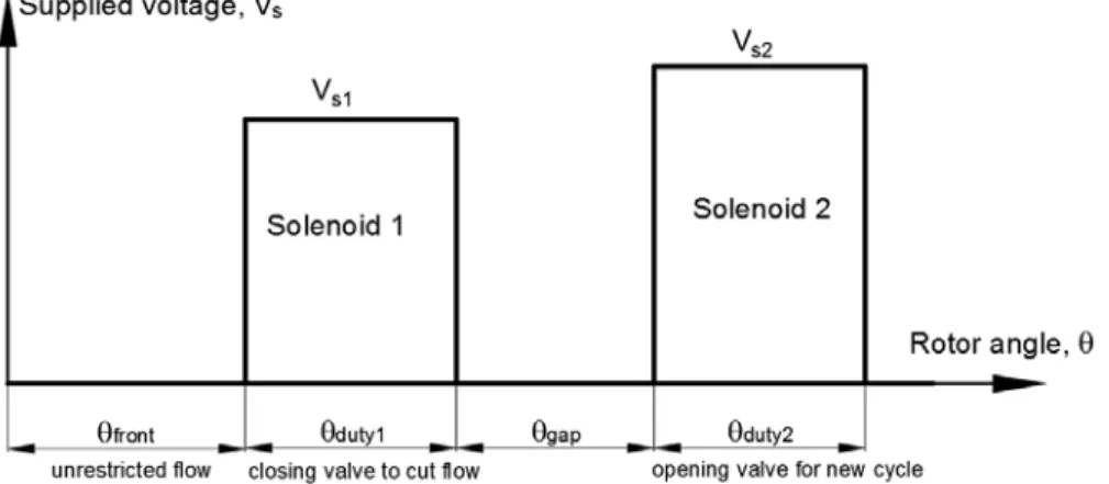
𝑧𝑧̇𝑚𝑚1 = 𝑏𝑏 𝑎𝑎 𝑧𝑧̇𝑣𝑣 𝑎𝑎𝑛𝑛𝑎𝑎 𝑧𝑧̇𝑚𝑚2=− 𝑏𝑏 𝑎𝑎 𝑧𝑧̇𝑣𝑣 [29] The solenoids are controlled based on the angular position of the rotor. When the inlet valve is required to be opened or closed at a certain rotor angular position, 𝜃𝜃, a electrical voltage is applied to the opening or closing solenoids. Before the solenoids can effectively close or open the inlet valve, current flow within the coils need time to build up. This current build-up can be derived from the relationship between voltage and current as follows:

𝑉𝑉𝑚𝑚1 =𝑖𝑖𝑚𝑚1𝑅𝑅𝑚𝑚1− 𝑖𝑖𝑚𝑚1𝛽𝛽𝑚𝑚 �𝑧𝑧𝑚𝑚1+𝑎𝑎0𝑔𝑔� 2𝑧𝑧̇𝑚𝑚1+ 𝛽𝛽𝑚𝑚 𝑧𝑧𝑚𝑚1+𝑎𝑎0𝑔𝑔 𝑎𝑎𝑖𝑖𝑚𝑚1 𝑎𝑎𝑡𝑡 [30] which can be rearranged for the change of current with respect to time as:

𝑎𝑎𝑖𝑖_𝑔𝑔1 𝑎𝑎𝑡𝑡 = 𝑧𝑧𝑚𝑚1+𝑎𝑎0𝑔𝑔 𝛽𝛽𝑚𝑚 �𝑉𝑉𝑚𝑚1− 𝑖𝑖𝑚𝑚1𝑅𝑅𝑚𝑚+ 𝛽𝛽𝑚𝑚𝑖𝑖𝑚𝑚1𝑧𝑧̇𝑚𝑚1 �𝑧𝑧𝑚𝑚1+𝑎𝑎0𝑔𝑔� 2� [31] Similarly, the build-up of current in the second solenoid can be expressed as:

𝑎𝑎𝑖𝑖_𝑔𝑔2 𝑎𝑎𝑡𝑡 = 𝑧𝑧𝑚𝑚2+𝑎𝑎0𝑔𝑔 𝛽𝛽𝑚𝑚 �𝑉𝑉𝑚𝑚2− 𝑖𝑖𝑚𝑚2𝑅𝑅𝑚𝑚+ 𝛽𝛽𝑚𝑚𝑖𝑖𝑚𝑚2𝑧𝑧̇𝑚𝑚2 �𝑧𝑧𝑚𝑚2+𝑎𝑎0𝑔𝑔� 2� [32] The nonlinear differential equations given by [27], [31], and [32] can be solved simultaneously in an iterative fashion to calculate the valve position and the solenoid currents at every rotor angle, 𝜃𝜃. The voltages that drive the

solenoids are given as shown in Figure 6 below to open and close the inlet valve at angles which are meant to match the power requirements of the expander for a given demand.

The effective orifice area or the equivalent area of the valve that allows the fluid to flow through during the valve opening phase can be calculated based on a simplified version of Hunt and Davis’s equation as follows (Tuymer & Machu, 2001): 𝐴𝐴𝑛𝑛𝑒𝑒 =� 1 1 (0.85𝜋𝜋𝜌𝜌𝑔𝑔(𝑚𝑚𝑔𝑔𝑠𝑠−𝑧𝑧𝑣𝑣))2+ 1 𝐴𝐴𝑣𝑣2 [33] where 𝐴𝐴_𝑣𝑣 =𝜋𝜋

4𝐷𝐷𝑚𝑚2 and 𝐷𝐷𝑚𝑚 is the diameter of the valve seat.

The thermodynamic model of limaçon machine is detailed in the next section.

The thermodynamic model

The performance of a limaçon-to-circular machine depends on the derivative 𝑎𝑎𝑉𝑉𝑛𝑛𝑛𝑛𝑡𝑡_𝑏𝑏

𝑎𝑎𝜃𝜃 , which can be expressed as: 𝑎𝑎𝑉𝑉𝑛𝑛𝑛𝑛𝑡𝑡𝑏𝑏

𝑎𝑎𝜃𝜃 = 4𝑏𝑏𝐻𝐻𝐿𝐿2sin𝜃𝜃

[34]

where 𝑉𝑉_{𝑛𝑛𝑛𝑛𝑡𝑡_𝑏𝑏} is volume of the working chamber below the rotor chord previously described in equation [2]. Hence, the mass flow rate, 𝑚𝑚

̇

= 𝑎𝑎𝑚𝑚

𝑎𝑎𝑡𝑡, of the fluid inside the working chamber in relation with the fluid density, the available

chamber volume, and the rotor angular position can be obtained as: Figure 6: Solenoid control voltage

𝑎𝑎𝑚𝑚 𝑎𝑎𝑡𝑡 =

�

4𝑏𝑏𝜌𝜌𝐻𝐻𝐿𝐿2sin𝜃𝜃+𝑉𝑉𝑛𝑛𝑛𝑛𝑡𝑡𝑏𝑏 𝑎𝑎𝜌𝜌 𝑎𝑎𝜃𝜃

�

𝑎𝑎𝜃𝜃 𝑎𝑎𝑡𝑡 =

�

4𝑏𝑏𝜌𝜌𝐻𝐻𝐿𝐿2sin𝜃𝜃+𝑉𝑉𝑛𝑛𝑛𝑛𝑡𝑡𝑏𝑏 𝑎𝑎𝜌𝜌 𝑎𝑎𝜃𝜃

�

𝜔𝜔 [35] where 𝜌𝜌, and 𝑚𝑚 are in turn the instantaneous density and mass of the fluid inside the working chamber at any given rotor angle 𝜃𝜃. The term 𝑎𝑎𝜃𝜃

𝑎𝑎𝑡𝑡= 𝜔𝜔 is the rotor angular velocity given in 𝑟𝑟𝑎𝑎𝑎𝑎

𝑠𝑠 . The change of the fluid mass in the working

chamber below the rotor chord can be obtained by rearranging equation [35] as follows:

𝑎𝑎𝜌𝜌_𝑏𝑏 𝑎𝑎𝜃𝜃 = 1 𝑉𝑉𝑛𝑛𝑛𝑛𝑡𝑡_𝑏𝑏

�

1 𝜔𝜔 𝑎𝑎𝑚𝑚 𝑎𝑎𝑡𝑡 −4𝑏𝑏𝜌𝜌𝑏𝑏𝐻𝐻𝐿𝐿2𝑠𝑠𝑖𝑖𝑛𝑛 𝜃𝜃

�

[36] where the subscript 𝑏𝑏 denotes “below the rotor”.

When the continuity equation is utilised and the effect of leakage through the sides of the machine and the apex seals are taken into account, equation [36] can then be re-written for the change of fluid mass in the two chambers below and above the rotor chord, respectively, as:

𝑎𝑎𝜌𝜌_𝑏𝑏 𝑎𝑎𝜃𝜃 = 1 𝑉𝑉_{𝑛𝑛𝑛𝑛𝑡𝑡_𝑏𝑏}

�

1 𝜔𝜔

�

𝐴𝐴𝑖𝑖𝑏𝑏𝜌𝜌𝑖𝑖𝑎𝑎𝑏𝑏𝑈𝑈𝑖𝑖𝑏𝑏− 𝐴𝐴𝑜𝑜𝑏𝑏𝜌𝜌𝑜𝑜𝑎𝑎𝑏𝑏𝑈𝑈𝑜𝑜𝑏𝑏− 𝑚𝑚

̇

𝑠𝑠𝑏𝑏±𝑚𝑚

̇

𝑎𝑎𝑠𝑠𝑏𝑏

�

−4𝑏𝑏𝜌𝜌𝑏𝑏𝐻𝐻𝐿𝐿2𝑠𝑠𝑖𝑖𝑛𝑛 𝜃𝜃

�

[37] 𝑎𝑎𝜌𝜌_𝑎𝑎 𝑎𝑎𝜃𝜃 = 1 𝑉𝑉𝑛𝑛𝑛𝑛𝑡𝑡_𝑎𝑎

�

1 𝜔𝜔

�

𝐴𝐴𝑖𝑖𝑎𝑎𝜌𝜌𝑖𝑖𝑎𝑎𝑎𝑎𝑈𝑈𝑖𝑖𝑎𝑎− 𝐴𝐴𝑜𝑜𝑎𝑎𝜌𝜌𝑜𝑜𝑎𝑎𝑎𝑎𝑈𝑈𝑜𝑜𝑎𝑎− 𝑚𝑚

̇

𝑠𝑠𝑎𝑎∓ 𝑚𝑚

̇

𝑎𝑎𝑠𝑠𝑎𝑎

�

−4𝑏𝑏𝜌𝜌𝑎𝑎𝐻𝐻𝐿𝐿2𝑠𝑠𝑖𝑖𝑛𝑛 𝜃𝜃

�

[38] where subscripts 𝑖𝑖,𝑜𝑜,𝑎𝑎,𝑎𝑎, and 𝑏𝑏 denote “inlet”, “outlet”, “down-stream”, “above the rotor chord”, and “below the rotor chord”, respectively

𝑚𝑚

̇

𝑠𝑠 and 𝑚𝑚

̇

𝑎𝑎𝑠𝑠 are the mass flowrate of leakages of working fluid through the sides of the machine and apex

seals, respectively

The velocity of the fluid through the inlet and outlet ports, 𝑈𝑈_𝑖𝑖 and 𝑈𝑈_𝑜𝑜, can be calculated by utilising equation [13]. The signs ± show the directions of such leakages, which are governed by the instantaneous value of pressures in the upper and lower chambers.

When the energy transfers to and from the fluid inside the working chamber is considered to occur as an adiabatic process, the following equation can be utilised:

𝑎𝑎ℎ𝑖𝑖 𝑎𝑎𝑡𝑡 − 𝑎𝑎ℎ𝑜𝑜 𝑎𝑎𝑡𝑡 = 𝑎𝑎

(

𝑚𝑚𝑛𝑛

)

𝑎𝑎𝑡𝑡 + 𝑃𝑃𝑎𝑎𝑉𝑉 𝑎𝑎𝑡𝑡 [39]

where ℎ_𝑖𝑖, and ℎ_𝑜𝑜 are the total enthalpy moving in and out of a working chamber, respectively; 𝑛𝑛 is the specific internal energy available in the working chamber. Since, the term internal energy, 𝑛𝑛, can be substituted by ℎ − 𝑝𝑝𝑣𝑣, and 𝑚𝑚𝑑𝑑ℎ

𝑑𝑑𝑛𝑛 =𝑚𝑚𝑚𝑚 𝑑𝑑𝑚𝑚 𝑑𝑑𝑛𝑛+𝑉𝑉

𝑑𝑑𝑑𝑑

𝑑𝑑𝑛𝑛, equation [39] can be re-written as: 𝑎𝑎ℎ𝑖𝑖 𝑎𝑎𝑡𝑡 − 𝑎𝑎ℎ𝑜𝑜 𝑎𝑎𝑡𝑡 = 𝑚𝑚𝑚𝑚𝑎𝑎𝑠𝑠 𝑎𝑎𝑡𝑡 + ℎ𝑎𝑎𝑚𝑚 𝑎𝑎𝑡𝑡 [40] or 𝑚𝑚𝑚𝑚𝜔𝜔𝑑𝑑𝑚𝑚 𝑑𝑑𝑑𝑑= (ℎ𝑖𝑖− ℎ) 𝑑𝑑𝑚𝑚𝑙𝑙 𝑑𝑑𝑛𝑛 −(ℎ𝑓𝑓− ℎ) 𝑑𝑑𝑚𝑚𝑜𝑜 𝑑𝑑𝑛𝑛 [41] The above equation can then be manipulated to produce equations, which show the rate of entropy change in the two working chambers per rotor angular rotational angle as below:

𝑎𝑎𝑠𝑠𝑏𝑏 𝑎𝑎𝜃𝜃 = 1 𝜔𝜔𝜌𝜌_𝑏𝑏𝑉𝑉𝑏𝑏𝑚𝑚𝑏𝑏

�

𝐴𝐴𝑖𝑖𝑏𝑏𝑈𝑈𝑖𝑖𝑏𝑏𝜌𝜌𝑖𝑖𝑎𝑎𝑏𝑏

(

ℎ𝑖𝑖𝑢𝑢𝑏𝑏− ℎ𝑏𝑏

)

− 𝐴𝐴𝑜𝑜𝑏𝑏𝑈𝑈𝑜𝑜𝑏𝑏𝜌𝜌𝑜𝑜𝑎𝑎𝑏𝑏

(

ℎ𝑜𝑜𝑢𝑢𝑏𝑏− ℎ𝑏𝑏

)

− 𝑚𝑚

̇

𝑠𝑠𝑏𝑏

(

ℎ𝑠𝑠𝑏𝑏− ℎ𝑏𝑏

)

±𝑚𝑚

̇

𝑎𝑎𝑠𝑠𝑏𝑏

(

ℎ𝑎𝑎𝑠𝑠𝑏𝑏− ℎ𝑏𝑏

)

�

[42] 𝑎𝑎𝑠𝑠𝑎𝑎 𝑎𝑎𝜃𝜃 = 1 𝜔𝜔𝜌𝜌_𝑎𝑎𝑉𝑉𝑎𝑎𝑚𝑚𝑎𝑎

�

𝐴𝐴𝑖𝑖𝑎𝑎𝑈𝑈𝑖𝑖𝑎𝑎𝜌𝜌𝑖𝑖𝑎𝑎𝑎𝑎

(

ℎ𝑖𝑖𝑢𝑢𝑎𝑎− ℎ𝑎𝑎

)

− 𝐴𝐴𝑜𝑜𝑎𝑎𝑈𝑈𝑜𝑜𝑎𝑎𝜌𝜌𝑜𝑜𝑎𝑎𝑎𝑎

(

ℎ𝑜𝑜𝑢𝑢𝑎𝑎− ℎ𝑎𝑎

)

− 𝑚𝑚

̇

𝑠𝑠𝑎𝑎

(

ℎ𝑠𝑠𝑎𝑎− ℎ𝑏𝑏

)

∓ 𝑚𝑚

̇

𝑎𝑎𝑠𝑠𝑎𝑎

(

ℎ𝑎𝑎𝑠𝑠𝑎𝑎 − ℎ𝑎𝑎

)

�

[43] where the subscripts 𝑖𝑖,𝑜𝑜,𝑎𝑎,𝑢𝑢,𝑎𝑎, and 𝑏𝑏 denote “inlet”, “outlet”, “down-stream”, “up-stream”, “above the rotor chord”, and “below the rotor chord”, respectively

𝑚𝑚𝑠𝑠 and 𝑚𝑚𝑎𝑎𝑠𝑠 are the mass flowrate of leakages of working fluid through the sides of the machine and apex

seals

ℎ𝑠𝑠 and ℎ𝑎𝑎𝑠𝑠 are the enthalpy on the upstream side of the sides and apex seals

Equations [37], [38], [42], and [43] can be solved simultaneously to the find the instantaneous values of densities, and entropies below and above the rotor chord, 𝜌𝜌_𝑏𝑏,𝜌𝜌_𝑎𝑎,𝑠𝑠_𝑏𝑏, and 𝑠𝑠_𝑎𝑎, of fluid in the two working chambers at each crank angle, 𝜃𝜃. At each calculation step, the corresponding values of pressure, 𝑃𝑃, density, 𝜌𝜌, and viscosity, 𝜇𝜇, can be calculated using the above equations. The instantaneous values for temperature, 𝑚𝑚, and enthalpy, ℎ, can be calculated with the assistance of the functions 𝑚𝑚(𝑃𝑃,𝑠𝑠), and ℎ(𝑃𝑃,𝑠𝑠) offered in REFPROP, which can be linked to

Matlab for fluid properties calculation (Lemmon, Huber, & McLinden, 2010; National Institute of Standards and Technology, 2016). The REFPROP functions deliver the fluid properties for not only single but also two-phase flows that are accurate enough for the calculations in this paper. In order to achieve further accuracy for the speed of sound in two-phase flow, the REFPROP functions has been utilised in conjunction with the algorithm offered in the published work by Lund and Flatten (2010).

In this paper, the authors investigate one of the embodiments of the limaçon machines; hence, the instantaneous crankshaft torque value can be calculated based on the equation suggested by Sultan (2005) as shown below:

𝜏𝜏= 4𝑏𝑏𝐿𝐿2_{𝐻𝐻(𝑃𝑃}

𝑐𝑐𝑏𝑏− 𝑃𝑃𝑐𝑐𝑚𝑚)sin𝜃𝜃

[44] where the subscript 𝑐𝑐,𝑏𝑏, and 𝑎𝑎 are “chamber”, “below the rotor”, and “above the rotor” respectively.

The calculation process for the machine crankshaft torque has been approached iteratively by applying the thermodynamic model and compute at small crank angle increments within the range 𝜃𝜃_{𝑙𝑙𝑖𝑖} ≤ 𝜃𝜃 ≤ 𝜃𝜃_{𝑙𝑙𝑖𝑖} +𝜋𝜋 in which the

𝜃𝜃𝑙𝑙𝑖𝑖 is angular position of the inlet port leading edge. The values of pressure and density below the rotor at the start of

the cycle, 𝑃𝑃_{𝑐𝑐𝑏𝑏}

(

𝜃𝜃_{𝑙𝑙𝑖𝑖}

)

and 𝜌𝜌_{𝑐𝑐𝑏𝑏}

(

𝜃𝜃_{𝑙𝑙𝑖𝑖}

)

, respectively, are compared with the corresponding values of pressure and density above the rotor chord at the end of the cycle, 𝑃𝑃_{𝑐𝑐𝑎𝑎}

(

𝜃𝜃_{𝑙𝑙𝑖𝑖}+𝜋𝜋

)

and 𝜌𝜌_{𝑐𝑐𝑎𝑎}

(

𝜃𝜃_{𝑙𝑙𝑖𝑖}+𝜋𝜋

)

. At the same time, the values of pressure and density above the rotor at the start of the cycle, 𝑃𝑃_{𝑐𝑐𝑎𝑎}

(

𝜃𝜃_{𝑙𝑙𝑖𝑖}

)

and 𝜌𝜌_{𝑐𝑐𝑎𝑎}

(

𝜃𝜃_{𝑙𝑙𝑖𝑖}

)

, respectively, are compared with the corresponding values of pressure and density below the rotor at the end of the cycle, 𝑃𝑃_{𝑐𝑐𝑏𝑏}

(

𝜃𝜃_{𝑙𝑙𝑖𝑖}+𝜋𝜋

)

and 𝜌𝜌_{𝑐𝑐𝑏𝑏}

(

𝜃𝜃_{𝑙𝑙𝑖𝑖}+𝜋𝜋

)

. The comparison process is done by using the dimensionless error expression shown below:

𝜖𝜖=��𝑃𝑃𝑐𝑐𝑏𝑏(𝜃𝜃𝑙𝑙𝑖𝑖)− 𝑃𝑃_𝑃𝑃𝑐𝑐𝑚𝑚(𝜃𝜃𝑙𝑙𝑖𝑖+𝜋𝜋) 𝑙𝑙 � � 2 +�𝜌𝜌𝑐𝑐𝑏𝑏(𝜃𝜃𝑙𝑙𝑖𝑖)− 𝜌𝜌_𝜌𝜌𝑐𝑐𝑚𝑚(𝜃𝜃𝑙𝑙𝑖𝑖+𝜋𝜋) 𝑙𝑙 � � 2 +�𝑃𝑃𝑐𝑐𝑚𝑚(𝜃𝜃𝑙𝑙𝑖𝑖)− 𝑃𝑃_𝑃𝑃𝑐𝑐𝑏𝑏(𝜃𝜃𝑙𝑙𝑖𝑖+𝜋𝜋) 𝑢𝑢 ��� � 2 +�𝜌𝜌𝑐𝑐𝑚𝑚(𝜃𝜃𝑙𝑙𝑖𝑖)− 𝜌𝜌_𝜌𝜌𝑐𝑐𝑏𝑏(𝜃𝜃𝑙𝑙𝑖𝑖+𝜋𝜋) 𝑢𝑢 ��� � 2 � 1/2 [45] where 𝑃𝑃

�

_𝑙𝑙= 𝑃𝑃𝑐𝑐𝑏𝑏(𝜃𝜃𝑙𝑙𝑖𝑖)+𝑃𝑃𝑐𝑐𝑎𝑎(𝜃𝜃𝑙𝑙𝑖𝑖+𝜋𝜋) 2 ,𝜌𝜌

�

𝑙𝑙 = 𝜌𝜌_{𝑐𝑐𝑏𝑏}(𝜃𝜃𝑙𝑙𝑖𝑖)+𝜌𝜌_{𝑐𝑐𝑎𝑎}(𝜃𝜃𝑙𝑙𝑖𝑖+𝜋𝜋) 2 ,𝑃𝑃

���

𝑢𝑢 = 𝑃𝑃𝑐𝑐𝑎𝑎(𝜃𝜃𝑙𝑙𝑖𝑖)+𝑃𝑃𝑐𝑐𝑏𝑏(𝜃𝜃𝑙𝑙𝑖𝑖+𝜋𝜋) 2 , and 𝜌𝜌

�

𝑢𝑢 = 𝜌𝜌_{𝑐𝑐𝑎𝑎}(𝜃𝜃𝑙𝑙𝑖𝑖)+𝜌𝜌_{𝑐𝑐𝑏𝑏}(𝜃𝜃𝑙𝑙𝑖𝑖+𝜋𝜋) 2 are the pressure and density coefficients used to calculate the error.

If the value of error expression, 𝜖𝜖, is larger than a small value defined by the designer, the values of

𝜋𝜋

)

,𝑎𝑎𝑛𝑛𝑎𝑎𝜌𝜌_{𝑐𝑐𝑏𝑏}

(

𝜃𝜃𝑙𝑙𝑖𝑖+𝜋𝜋

)

, respectively. The calculation process is then repeated over the range of 𝜃𝜃 ∈[𝜃𝜃𝑙𝑙𝑖𝑖,𝜃𝜃𝑙𝑙𝑖𝑖+𝜋𝜋] until

the outcome of the error expression falls below the predefined value, which reflects the cyclical nature of the thermodynamic process. Once the convergence is achieved, the total energy per one cycle, 𝑃𝑃_{𝑐𝑐𝑦𝑦𝑐𝑐𝑙𝑙𝑛𝑛}, can calculated by utilising the following equation:

𝑃𝑃𝑐𝑐𝑦𝑦𝑐𝑐𝑙𝑙𝑛𝑛 = 2 𝛿𝛿𝜃𝜃

��

𝜏𝜏𝑠𝑠𝑛𝑛 𝑁𝑁 𝑛𝑛=1 −𝜏𝜏𝑠𝑠𝑛𝑛+𝜏𝜏𝑠𝑠1 2

�

[46] where 𝛿𝛿𝜃𝜃 is the size of the angular interval, 𝑛𝑛 ∈[1,𝑁𝑁] is the counter for the successive points on the torque curve, and N is the total number of intervals on the torque curve.

With the same approach, the total mass flow through the machine in one cycle, 𝑀𝑀_{𝑐𝑐𝑦𝑦𝑐𝑐𝑙𝑙𝑛𝑛}, can be calculated using the expression below:

𝑀𝑀𝑐𝑐𝑦𝑦𝑐𝑐𝑙𝑙𝑛𝑛 = 2𝛿𝛿𝜃𝜃_𝜔𝜔

�� ��

𝐴𝐴𝑖𝑖𝑏𝑏𝜌𝜌_{𝑖𝑖𝑎𝑎𝑏𝑏}𝑈𝑈𝑖𝑖𝑏𝑏

�

_𝑛𝑛+

�

𝐴𝐴𝑖𝑖𝑎𝑎𝜌𝜌_{𝑖𝑖𝑎𝑎𝑎𝑎}𝑈𝑈𝑖𝑖𝑎𝑎

�

_𝑛𝑛

�

𝑁𝑁 𝑛𝑛=1 −

�

𝐴𝐴𝑖𝑖𝑏𝑏𝜌𝜌𝑖𝑖𝑎𝑎𝑏𝑏𝑈𝑈𝑖𝑖𝑏𝑏

�

𝑛𝑛+

�

𝐴𝐴𝑖𝑖𝑏𝑏𝜌𝜌𝑖𝑖𝑎𝑎𝑏𝑏𝑈𝑈𝑖𝑖𝑏𝑏

�

1 2 −

�

𝐴𝐴𝑖𝑖𝑎𝑎𝜌𝜌𝑖𝑖𝑎𝑎𝑎𝑎𝑈𝑈𝑖𝑖𝑎𝑎

�

𝑛𝑛+

�

𝐴𝐴𝑖𝑖𝑎𝑎𝜌𝜌𝑖𝑖𝑎𝑎𝑎𝑎𝑈𝑈𝑖𝑖𝑎𝑎

�

1 2

�

[47] The machine overall efficiency can be calculated from the total energy per one cycle and total mass flow through the machine as follows:

𝜂𝜂𝑓𝑓=_𝑀𝑀𝑃𝑃𝑐𝑐𝑦𝑦𝑐𝑐𝑙𝑙𝑛𝑛 𝑐𝑐𝑦𝑦𝑐𝑐𝑙𝑙𝑛𝑛∆ℎ𝑖𝑖𝑚𝑚

[48] where ∆ℎ_{𝑖𝑖𝑚𝑚} is the difference between the enthalpy in the inlet manifold and its isentropically reduced value in the discharge manifold. It should be highlighted that in order to account for the fact that for each full rotation of the shaft, the limaçon-to-circular machine has two fluid expanding cycles, hence, a multiplication by two is incorporated in equations [46] and [47].

Numerical illustrations

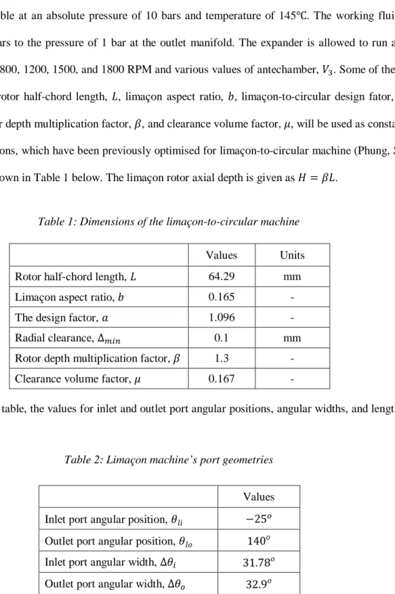
The study of this limaçon-to-circular expander utilises organic gas 245fa as a working fluid. Saturated R-245fa is made available at an absolute pressure of 10 bars and temperature of 145℃. The working fluid will be expanded from 10 bars to the pressure of 1 bar at the outlet manifold. The expander is allowed to run at various angular velocity i.e.: 800, 1200, 1500, and 1800 RPM and various values of antechamber, 𝑉𝑉₃. Some of the machine dimensions such as rotor half-chord length, 𝐿𝐿, limaçon aspect ratio, 𝑏𝑏, limaçon-to-circular design fator, 𝑎𝑎, radial clearance, Δ_{𝑚𝑚𝑖𝑖𝑛𝑛}, rotor depth multiplication factor, 𝛽𝛽, and clearance volume factor, 𝜇𝜇, will be used as constant in this study. These dimensions, which have been previously optimised for limaçon-to-circular machine (Phung, Sultan, & Boretti, 2016), are shown in Table 1 below. The limaçon rotor axial depth is given as 𝐻𝐻=𝛽𝛽𝐿𝐿.

In the following table, the values for inlet and outlet port angular positions, angular widths, and lengths are set as:

A representation of chamber pressure and temperature against the crank angle, 𝜃𝜃, and the pressure-volume relationship can be found in Figure 7 and Figure 8 as below:

Values Units Rotor half-chord length, 𝐿𝐿 64.29 mm Limaçon aspect ratio, 𝑏𝑏 0.165 - The design factor, 𝑎𝑎 1.096 - Radial clearance, Δ_{𝑚𝑚𝑖𝑖𝑛𝑛} 0.1 mm Rotor depth multiplication factor, 𝛽𝛽 1.3 - Clearance volume factor, 𝜇𝜇 0.167 -

Values Inlet port angular position, 𝜃𝜃_{𝑙𝑙𝑖𝑖} −25𝑓𝑓 Outlet port angular position, 𝜃𝜃_{𝑙𝑙𝑜𝑜} 140𝑜𝑜 Inlet port angular width, Δ𝜃𝜃_𝑖𝑖 31.78𝑜𝑜 Outlet port angular width, Δ𝜃𝜃_𝑓𝑓 32.9𝑜𝑜 Inlet port length, 𝐿𝐿_𝑜𝑜 71 𝑚𝑚𝑚𝑚 Outlet port length, 𝐿𝐿_𝑖𝑖 107 𝑚𝑚𝑚𝑚

Table 2: Limaçon machine’s port geometries Table 1: Dimensions of the limaçon-to-circular machine

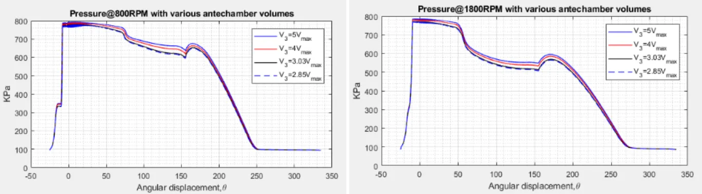
Volume of the antechamber, 𝑉𝑉₃, also affect the pressure within the machine working chamber as shown in Figure 9. When volume of antechamber is small, pressure inside the machine working chamber tends to drop further compared to the case where antechamber volume is large. This is also true with the temperature drop in the working chamber (Figure 9). The larger the antechamber gets, fluid supply to the limaçon machine is more sufficient which can help the machine utilising the pressure difference between the inlet and outlet more effectively. Moreover, increasing the antechamber volume, of course to a certain extent, also means that the inlet valve doesn’t need to stay open for a long period of time to supply working fluid; this effect will be shown later in this section.

The magnitude of solenoid voltages 𝑉𝑉_𝑚𝑚1 and 𝑉𝑉_𝑚𝑚2 can be set by the designer based on the operational condition of limaçon machine; here, these voltages were set equal as 𝑉𝑉_𝑚𝑚1 =𝑉𝑉_𝑚𝑚2=𝑉𝑉_𝑚𝑚= 75 𝑉𝑉𝑜𝑜𝑙𝑙𝑡𝑡. The valve opening and closing

Figure 7: Chamber pressure and temperature against crank angle

Figure 8: Limaçon machine PV diagram

with respect to rotor angular displacement at different RPMs and antechamber volumes are shown in Figure 10; of note is that the valve stroke is set at 5 𝑚𝑚𝑚𝑚 (Figure 10).

In this design, the valve is fully open when valve motion, 𝑧𝑧_𝑣𝑣 = 0; when 𝑧𝑧_𝑣𝑣= 5 𝑚𝑚𝑚𝑚, the valve is fully closed. Figure 10 shows the valve action with the help from solenoids at various angular velocities. It is worth noting that when voltage is supplied to the coils, the solenoid currents need to build-up before the solenoids can jump into action to close the valve and cut off fluid supply or assist the valve spring in the vale opening phase. Such current build-ups are shown in Figure 11. Obviously, the valve displacement, 𝑧𝑧_𝑣𝑣, increases or decreases gradually

according to solenoid responses. Figure 10 also shows that the valve can stay open for a much longer period at lower RPM – shown as solid blue curve – compared to higher RPM – shown as red or solid black curve. This results in better fluid supply for the antechamber and consequently the machine working chamber. The solid magenta curve shown in Figure 10, in particular, is an indication that the inlet valve cannot achieve fully close position. This is due to the relatively slow response time of the solenoids compared to the machine angular velocity. This problem can be easily overcome when faster response time solenoids are used in limaçon machines that operate at higher RPM.

Figure 12 and Figure 13 show linear and angular magnitudes of the seal motion as well as the seal-housing forces at 800 and 1800 RPM, respectively. The forces exerted between the seal and housing when the machine runs at 1800 RPM is significantly higher than that of the 800 RPM. In fact, this behaviour is expected since at lower RPM the difference in pressure between the machine chamber and the outlet is much greater as shown in Figure 9. This pressure difference tends to push the seal against one side of the seal groove and help reducing both linear and angular

Figure 10: Valve opening against rotor angle at various RPM and 𝑉𝑉₃

Figure 11: Solenoid currents at one particular RPM

displacement of the seal. At higher RPM, the centrifugal force on the seal together with the lower in pressure difference have seen seal motion inside the seal groove and housing force increasing. Such an increase in seal-housing force will result in higher friction force between the seal tip and the machine seal-housing surface which will adversely affect the machine performance. Hence it is critical to find an optimum seal spring stiffness, inlet valve settings, volume of antechamber, and RPM to maximise the machine output power.

The overall efficiencies of the limaçon machine at different RPM and values of antechamber 𝑉𝑉₃, as shown in Figure 14, can be calculated using equations [46], [47], and [48]. It is worth noting that although the amount of friction loss between seal and housing increases with the increase

of RPM, the overall efficiency of the machine improves significantly at higher speed.

Figure 12: Seal displacements and seal-housing force @800 RPM and 𝑉𝑉₃= 2.85 𝑉𝑉_{𝑚𝑚𝑚𝑚𝑥𝑥}

Figure 13: Seal displacements and seal-housing force @1800 RPM and 𝑉𝑉₃= 2.85 𝑉𝑉_{𝑚𝑚𝑚𝑚𝑥𝑥}

Conclusion

This paper investigates the thermodynamic performance of the limaçon-to-circular machines; the inlet and outlet ports’ angular positions, angular widths, and lengths of the limaçon-to-circular machines have been previously optimised based on the operational condition. The seal dynamic models as well as the inlet valve dynamics response have been taken into account to demonstrate and compare the effectiveness and efficiency of the machine due to sealing and inlet valve inclusion. Future work on limaçon machine optimisation can be done with the incorporation of apex seal and inlet valve dynamics.

Nomenclatures

2𝐿𝐿 : the limaçon chord length

𝑋𝑋𝑋𝑋 : stationary frame

𝑋𝑋𝑟𝑟𝑋𝑋𝑟𝑟: moving frame 𝑜𝑜 : limaçon pole

𝑝𝑝_𝑙𝑙,𝑝𝑝_𝑡𝑡: leading and trailing apices

𝜃𝜃 : crank angle

𝑟𝑟 : radius of the base circle

𝑚𝑚 : centre point of the chord

𝑅𝑅 : radius of the circular segment

𝐶𝐶 : clearance value

𝑏𝑏 : limaçon aspect ratio

𝑉𝑉𝑛𝑛𝑛𝑛𝑡𝑡: volume of the working chamber 𝐻𝐻 : the expander’s housing depth

𝑹𝑹𝑙𝑙,𝑹𝑹𝑡𝑡: position vector of the ports’ leading and trailing edges 𝑹𝑹

�

_𝑙𝑙,𝑹𝑹

�

𝑡𝑡: leading and trailing unit vectors

𝐿𝐿𝑝𝑝 : port length 𝑊𝑊 : port width

𝐴𝐴𝑓𝑓 : cross sectional area of the port 𝐴𝐴𝑝𝑝 : instantaneous value of the port area

𝑷𝑷𝑙𝑙,𝑷𝑷𝑡𝑡: position of the rotor’s leading and trailing edges 𝑿𝑿

�

_𝑟𝑟 : unit vector along the rotor chord

𝒀𝒀

�

_𝑟𝑟 : unit vector along the axis perpendicular to the rotor chord

𝑠𝑠𝑙𝑙,𝑠𝑠𝑡𝑡: relative locations of the rotor leading and trailing apices with respect to the port leading and trailing edges 𝑈𝑈 : velocity of the fluid

ℎ𝑢𝑢,ℎ𝑎𝑎: upstream and downstream isentropic enthalpy Δℎ : isentropic enthalpy drop along the flow direction

𝐾𝐾𝑝𝑝 : the loss coefficient 𝑓𝑓 : friction factor

𝑅𝑅𝑛𝑛 : Reynolds number

𝜌𝜌 : density of the working fluid

𝜇𝜇 : viscosity

𝑥𝑥 : dryness fraction

𝑚𝑚

̇

: mass flow rate

𝜏𝜏 : crankshaft torque

𝜖𝜖 : error expression used to end the cyclical iteration

Φ : design vector

𝛿𝛿𝜃𝜃 : size of the angular interval

𝑀𝑀𝑐𝑐𝑦𝑦𝑐𝑐𝑙𝑙𝑛𝑛: total mass flow per cycle 𝜔𝜔 : angular velocity of the rotor

𝑚𝑚1,𝑚𝑚2,𝑚𝑚3: mass of the plunger, the lever, and the inlet valve

𝑘𝑘𝑣𝑣,𝑘𝑘𝑚𝑚𝑛𝑛𝑓𝑓𝑝𝑝,𝑘𝑘𝑚𝑚𝑛𝑛𝑚𝑚𝑛𝑛: stiffness of the valve spring, the mechanical stopper, and the seat 𝑐𝑐𝑚𝑚𝑛𝑛𝑚𝑚𝑛𝑛,𝑐𝑐𝑚𝑚𝑛𝑛𝑓𝑓𝑝𝑝: damping coefficient of the seat and mechanical stopper

𝛿𝛿𝑣𝑣 : valve spring initial deflection

𝐼𝐼2 : moment of inertia of the lever about the pivot point 𝑥𝑥𝑣𝑣,𝑦𝑦𝑣𝑣,𝑧𝑧𝑣𝑣: displacement of the plunger, lever, and valve 𝑥𝑥̇𝑣𝑣,𝑦𝑦̇𝑣𝑣,𝑧𝑧̇𝑣𝑣: velocity of the pluger, lever, and valve 𝑧𝑧̈𝑣𝑣 : acceleration of the valve

𝐹𝐹𝑚𝑚𝑙𝑙 : force exerted by the solenoids

𝐹𝐹𝑚𝑚𝑢𝑢𝑟𝑟: contact force that the valve experiences 𝑉𝑉3 : volume of the antechamber

Δ𝑃𝑃 : difference in pressure between the inlet and antechamber

𝐴𝐴𝑣𝑣 : area of the vale that is subjected to the effect of pressure difference 𝑖𝑖𝑚𝑚𝑙𝑙 : solenoid currents

𝑉𝑉𝑚𝑚𝑙𝑙 : solenoid supplied voltage

𝑧𝑧𝑚𝑚𝑙𝑙 : displacements of the plunger relative to the solenoids 1 and 2

References

Climate Council. (2015). Climate change 2015: Growing risks, critical choices. Climate Council of Australia

Ltd. Australia: Climate Council of Australia Ltd.

Department of Industry and Science. (2015). Australian Energy Update. Department of Industry and Science. Canberra: Department of Industry and Science. http://www.industry.gov.au/Office-of-the-Chief-Economist/Publications/Documents/aes/2015-australian-energy-statistics.pdf

Dunn, W., & Shultis, J. (2012). Exploring Monte Carlo methods. Amsterdam: Elsevier/Academic Press. Fairhurst, C. (1983). Component pressure loss during two-phase flow. International conference on the Physical modelling of multi-phase flow, 1-24.

International Energy Agency. (2015). Key world energy statistics. OECD/International Energy Agency. Paris: International Energy Agency.

IPCC. (2015). Climate change 2014 - Synthesis report. Intergovernmental panel on climate change. Switzerland: Intergovernmental panel on climate change. https://www.ipcc.ch/pdf/assessment-report/ar5/syr/SYR_AR5_FINAL_full_wcover.pdf

Lemmon, E. W., Huber, M. L., & McLinden, M. O. (2010). NIST Reference Fluid Thermodynamic and Transport Properties—REFPROP Version 9.0. Gaithersburg, Maryland 20899: U.S. Department of Commerce - Technology Administration - National Institute of Standards and Technology.

Lemort, V., Quoilin, S., Cuevas, C., & Lebrun, J. (2009). Testing and modeling a scroll expander integrated into an Organic Rankine Cycle. Applied Thermal Engineering, 29(14-15), 3094-3102. doi: 10.1016/j.applthermaleng.2009.04.013

Lund, H., & Flatten, T. (2010). Equilibrium conditions and sound velocities in two-phase flows. SIAM Annual Meeting (AN10). Pittsburgh, Pennsylvania, USA.

Massoud, M. (2005). Engineering thermofluids - Thermodynamics, fluid mechanics and heat transfer. Berlin: Springer.

Mathias, J., Johnston, J., Cao, J., Priedeman, D., & Christensen, R. (2009). Experimental Testing of Gerotor and Scroll Expanders Used in, and Energetic and Exergetic Modeling of, an Organic Rankine Cycle. Journal Of Energy Resources Technology, 131(1), 012201. doi: 10.1115/1.3066345

McNeil, D. (2000). Two-phase flow in orifice plates and valves. Proceedings Of The Institution Of Mechanical Engineers, Part C: Journal Of Mechanical Engineering Science, 214(5), 743-756. doi: 10.1243/0954406001523740

Munson, B., Okiishi, T., Huebsch, W., & Rothmayer, A. (2013). Fundamentals of fluid mechanics. Hoboken, NJ: John Wiley & Sons, Inc.

National Institute of Standards and Technology. (2016, 03 02). Linking REFPROP with other applications. http://www.boulder.nist.gov/div838/theory/refprop/LINKING/Linking.htm#MatLabApplications

Phung, T. H., Sultan, I. A., & Boretti, A. (2016). Design of Limaçon Gas Expanders. In R. N. Jazar, & L. Dai (Eds.), Nonlinear Approaches in Engineering Applications, 91-120. Springer International Publishing Switzerland.

Ryley, D. (1964). Property definition in equilibrium wet steam. International Journal Of Mechanical Sciences, 6(6), 445-454. doi: 10.1016/s0020-7403(64)80005-9

Sultan, I. (2005). The Limaçon of Pascal: Mechanical Generation and Utilization for Fluid Processing. Proceedings Of The Institution Of Mechanical Engineers, Part C: Journal Of Mechanical Engineering Science, 219(8), 813-822. doi: 10.1243/095440605x31698

Sultan, I. (2008). A Geometric Design Model for the Circolimaçon Positive Displacement Machine. Journal Of Mechanical Design, 130(6), 062307. doi: 10.1115/1.2901143

Sultan, I. (2012). Optimum design of limaçon gas expanders based on thermodynamic performance. Applied Thermal Engineering, 39, 188-197. doi: 10.1016/j.applthermaleng.2012.01.039

Sultan, I., & Schaller, C. (2011). Optimum Positioning of Ports in the Limaçon Gas Expanders. Journal Of Engineering For Gas Turbines And Power, 133(10), 103002. doi: 10.1115/1.4003195

Tuymer, W. J., & Machu, E. H. (2001). Compressor valves. In P. C. Hanlon (Ed.), Compressor handbook, 20.1-20.29. New York: McGraw-Hill.

Yuan, Q., & Li, P. Y. (2004). Self-calibration of push-pull solenoid actuators in electrohydraulic valves. 2004 ASME International Mechanical Engineering Congress and RD&D Expo, 269-275. California: ASME. doi:10.1115/IMECE2004-62109