Discrete Ranked Set Sampling

(1)

Southern Methodist University

SMU Scholar

Statistical Science Theses and Dissertations Statistical Science

Spring 5-7-2018

Discrete Ranked Set Sampling

Heng Cui

Southern Methodist University, [email protected]

Follow this and additional works at:https://scholar.smu.edu/hum_sci_statisticalscience_etds

Part of theStatistical Methodology Commons

This Dissertation is brought to you for free and open access by the Statistical Science at SMU Scholar. It has been accepted for inclusion in Statistical Science Theses and Dissertations by an authorized administrator of SMU Scholar. For more information, please visithttp://digitalrepository.smu.edu. Recommended Citation

Cui, Heng, "Discrete Ranked Set Sampling" (2018).Statistical Science Theses and Dissertations. 2.

(2)

DISCRETE RANKED SET SAMPLING

Approved by:

Dr. Lynne Stokes Committee Chair

Dr. Min Chen

Dr. Hon Keung Tony Ng

Dr. Cornelis Jr. Potgieter

(3)

DISCRETE RANKED SET SAMPLING

A Dissertation Presented to the Graduate Faculty of the Dedman College

Southern Methodist University in

Partial Fulfillment of the Requirements for the degree of

Doctor of Philosophy with a

Major in Statistical Science by

Heng Cui

B.S., Information and Computational Science, Shandong University, China M.S., Financial Mathematics, Shandong University, China

(4)

Copyright (2018)

Heng Cui

(5)

ACKNOWLEDGMENTS

Completion of this dissertation is impossible without the supports of several people. First of all, I would like to thank my advisor, Dr. Lynne Stokes, for her encouragement, guidance, and supports through the last two years. Dr. Stokes has provided me so many insightful suggestions and advice to help me finish my dissertation. She also made me realize the importance of paying attention to detail. Her advice and careful editing improved this dissertation to another level.

I am extremely grateful for all valuable suggestions and concise comments from the other committee members- Dr. Tony, Dr. Potgieter, Dr. Sherry and Dr. Chen. Thank for your time and academic efforts to help me improve my dissertation. To Dr. Tony, Dr. Potgieter and Dr. Sherry, I was so lucky to take classes from you. Your expertise in Statistics has inspired me and helped me learn about the beauty of Statistics.

I would also like to express my thanks to all of my friends. Thank you for listening to me, offering me advice and supporting me throughout the journey.

Finally, I would like to acknowledge with gratitude, the support and love of my family-my parents, family-my brother and family-my wife. Thank you all for encouraging me in all of family-my pursuits and inspiring me to follow my dreams. You are the most important people to me in the world and I dedicate this dissertation to you.

(6)

Cui, Heng B.S., Information and Computational Science, Shandong University, China M.S., Financial Mathematics, Shandong University, China

Discrete Ranked Set Sampling

Advisor: Dr. Lynne Stokes

Doctor of Philosophy degree conferred May 7, 2018 Dissertation completed May 7, 2018

Ranked set sampling (RSS) is an efficient data collection framework compared to simple random sampling (SRS). It is widely used in various application areas such as agriculture, environment, sociology, and medicine, especially in situations where measurement is expen-sive but ranking is less costly. Most past research in RSS focused on situations where the underlying distribution is continuous. However, it is not unusual to have a discrete data generation mechanism. Estimating statistical functionals are challenging as ties may truly exist in discrete RSS. In this thesis, we started with estimating the cumulative distribution function (CDF) in discrete RSS. We proposed two methods to incorporate the information brought by ties. The first method is based on the idea ofFrey (2012), which only works for the balanced RSS. The second one is based on the NPMLE method proposed by Kvam and

Samaniego (1994). The second method can be applied in both balanced and unbalanced

RSS. By simulation studies, we showed that the new methods improve the efficiency of esti-mation. Later, we proposed the corresponding plug-in estimators for the population mean and the population variance. The new estimators showed higher efficiency compared to the existing estimators in the literature.

Another problem considered in this thesis is to improve the estimation efficiency of each order stratum CDF when tie information is not available. We proposed a new estimator by imposing uniformly stochastic ordering constraint on the order strata CDF’s. By using the ”ranking” relationship between the order strata CDF’s, the new estimator showed a higher efficiency for the strata except the edge strata (the smallest and largest order stratum).

(7)

TABLE OF CONTENTS

LIST OF FIGURES . . . viii

LIST OF TABLES . . . x

CHAPTER 1. INTRODUCTION . . . 1

1.1. Research Background . . . 1

1.2. Discrete Ranked Set Sampling Procedures and Variations . . . 2

1.3. Research Objectives . . . 4

2. ESTIMATORS OF THE CUMULATIVE DISTRIBUTION FUNCTION BY USING RSS . . . 5

2.1. Empirical Distribution Function . . . 5

2.2. Alternative to the EDF: Frey’s Estimator . . . 7

2.3. Nonparametric Maximum Likelihood Estimator of the CDF . . . 11

2.4. Resampling Methods for Ranked Set Sampling . . . 16

2.5. Simulation Study . . . 19

2.6. Conclusion . . . 23

3. ON ESTIMATING THE POPULATION MEAN . . . 24

3.1. Background . . . 24

3.2. Frey’s Estimator of the Population Mean . . . 26

3.3. Nonparametric Maximum Likelihood Estimator ofµ . . . 27

3.4.1. Performance of Estimators Under Balanced Discrete Ranked Set Sampling . . . 28

3.4.2. Performance of Estimators Under Unbalanced Discrete Ranked Set Sampling . . . 32

(8)

3.4.3. Inference on Population Mean . . . 35

4. ON ESTIMATING THE POPULATION VARIANCE . . . 40

4.1. Background . . . 40

4.2. New Estimators of Population Variance . . . 41

4.3.1. Comparison of Variance Estimators . . . 42

4.3.2. Inference on Population Variance . . . 47

5. ON ESTIMATING THE ORDER STRATUM CDF BY USING DISCRETE RANKED SET SAMPLING . . . 54

5.1. Literature Review . . . 54

5.2. Three Types of Stochastic Ordering . . . 55

5.3. Estimators under Ordinary Stochastic Ordering . . . 57

5.4. Estimating Under Uniformly Stochastic Ordering . . . 58

5.5. Simulation Studies . . . 59

5.6. Conclusions . . . 63

6. DISCUSSION AND FUTURE DIRECTIONS . . . 64

6.1. Ranking Error Models . . . 64

6.2. Variations of Ranked Set Sampling . . . 65

APPENDIX A. DISCRETE ORDER STATISTICS . . . 66

(9)

LIST OF FIGURES

Figure Page

2.1 RE of ˆpe_j for H = 2,3,4, and 5.. . . 7

2.2 Original samples and corresponding weights . . . 8

2.3 Relative efficiency of CDF estimators for discrete uniform distributions . . . 20

2.4 Relative efficiency of CDF estimators for binomial distributions . . . 21

2.5 Relative efficiency of CDF estimators for Poisson distributions . . . 22

3.1 Relative efficiency of mean estimators for discrete uniform distributions (N0).. . 29

3.2 Relative efficiency for binomial distributions (n= 10, p). . . 30

3.3 Relative efficiency of mean estimators for Poisson distributions (λ).. . . 31

3.4 Relative efficiency of mean estimators versus sampling proportion from 1st order stratum fordiscrete uniform(N0 = 5,10), Poisson(λ = 1,3) and binomial(n= 10, p=.2, .5) for H = 2. . . 33

4.1 Relative efficiency of population variance estimators for discrete uniform distributions (N0).. . . 44

4.2 Relative efficiency of population variance estimators for binomial distributions(n = 10, p).. . . 45

4.3 Relative efficiency for Poisson distributions (λ).. . . 46

4.4 Histogram of ˆσ_{N P M LE}2 when ranked set samples are generated from bino-mial(10, 0.5). The set size is 5 and the cycle size is 5.. . . 48

4.5 Coverage probability of confidence intervals produced by the bootstrap pro-cedure when ranked set samples or simple random samples generated for binomial(10,0.5) whenH = 5. For simple random sample, thex-axis denotes equivalent cycle size; that is the sample size divided byH. . . 51

5.1 Relative efficiency of ˆF_[i_r_](i=iso, uso) for discrete uniform distribution(N0). The number r on each line respresents r-th order stratum.. . . 61

(10)

5.2 Relative efficiency of ˆFi

[r](i =iso, uso) for binomial(n = 10, p) distribution.

The number r on each line respresents r-th order stratum.. . . 62

5.3 Relative efficiency of ˆFi

[r](i = iso, uso) for Poisson distribution (λ). The

(11)

LIST OF TABLES

Table Page

3.1 Relative Efficiency of ˆµRSS from a balanced discrete ranked-set sample for

some common discrete distributions . . . 25

3.2 Simulated bias, variance and MSE of mean estimators for Binomial (10, 0.2)

based on 10000 replicates (N = 30) . . . 35

3.3 Coverage probability, the average of estimates of the standard error of ˆ

µN P M LE_{, and the simulated standard error of ˆ}_µN P M LE _{based on 2000}

replicates. . . 38

4.1 Coverage probability, the average of standard error estimates of ˆσ_{N P M LE}2 , and the simulated standard error of ˆσ2

N P M LE based on 2000 replicates. . . 52

(12)

(13)

CHAPTER 1 INTRODUCTION

1.1. Research Background

Ranked set sampling (RSS) is an efficient data collection framework compared to simple random sampling (SRS). It is widely used in various application areas such as agriculture, en-vironment, sociology, and medicine, especially in situations where measurement is expensive but ranking is less costly.

RSS was first proposed by McIntyre (1952) for estimating mean pasture yields. It im-proved the efficiency of estimating the population mean by incorporating the investigators’ judgment. Takahasi and Wakimoto (1968) provided the theoretical foundations of RSS. They showed that the relative efficiency of the mean estimator by using RSS compared to SRS is bounded and the upper bound is achieved when the underlying distribution is a uniform distribution. Later, the research on ranked set sampling developed in two major directions. One direction of research on RSS was to estimate different parameters other than the mean, including the population variance, cumulative distribution function (CDF), quantile function, etc. For example, Stokes and Sager (1988) proposed the empirical distri-bution function (EDF) based on a ranked set sample. Kvam and Samaniego (1994) provided the nonparametric maximum likelihood estimator of the CDF, which was shown to be more precise compared to the EDF when no ranking error exist. Another direction of research was to consider the variations of the RSS design. One of the most important variations was judgement post-stratification (JPS) proposed byMacEachern et al. (2004). JPS attracted a lot of research because of its practical flexibilities.

(14)

mechanism. The only available literature considering the RSS with discrete underlying distributions isBarabesi and Pisani(2002). One important difference between discrete cases and continuous cases is that ties may truly exist in discrete cases. Frey (2012) discussed the perceived tie problem in continuous JPS. A perceived tie is declared if the ranker is not sure about the ranking between two units. Frey(2012) showed that using information about perceived ties can improve the relative efficiency of mean estimators. Later in this thesis, we will show their proposed estimator can be adapted into discrete RSS, where the perceived ties are actual ties.

1.2. Discrete Ranked Set Sampling Procedures and Variations

Generally, the process of selecting a ranked set sample can be briefly summarized as following:

First, draw a set of H sample units randomly from the population and then rank those units visually or by some inexpensive method. H is called the set size and usually set to be small (less than 10) in order to avoid ranking errors. The unit judged smallest is then chosen to be measured in an accurate way which may be expensive or time-consuming. Then repeat the same procedure until we get n1 units judged smallest to measure.

Similarly, we can sample nr units judged r-th (r= 2,· · ·, H) smallest to measure. After

measuring those units accurately, we get a ranked set sample. Let {X[r]i; r = 1,· · ·, H; i=

1,· · ·, nr} denote the ranked set sample, where X[r]i is the measured value of i-th unit with

rank r. If n1 = n2 = · · · = nH = n, the design is balanced and n is called cycle size.

An unbalanced ranked set sample differs from a balanced one in that the measured order statistics no longer must be included an equal number of times in the full sample, as long as units from each order stratum are included at least once. In the following discussion, let N

denote the sample size of a ranked set sample, i.e. N =PH

r=1nr.

The whole process is analogous to stratified sampling. Each order statistic is analogous to one stratum in stratified sampling. Therefore, a ranked set sample with set size H is similar to a stratified sample with H strata.

(15)

An important variation of ranked set sampling is judgment post-stratification (JPS) proposed by MacEachern et al.(2004). In JPS, a simple random sample of sizeN is selected and measured first. Then N sets of samples of size H −1 are selected to work as the comparison samples. JPS is similar to unbalanced RSS except that the sample size from each stratum is determined randomly by using a multinomial distribution, i.e. (n1,· · ·, nH)∼

M ultinomial(N;_H1,· · ·,_H1). Although JPS was shown to be less efficient than RSS, it still

attracted a lot of research attention because of its practical usefulness. Besides JPS, there were some other useful variations of RSS in the literature; seeAl-Saleh and Al-Kadiri(2000),

Al-Saleh and Al-Omari(2002), Hossain and Muttlak(1999), etc.

The main focus in this thesis is to consider the applications of RSS and its variations when the underlying distribution is discrete. So it is important to make clear the differences between discrete RSS and continuous RSS first. The main difference is in the ranking process. In continuous RSS, the rankers should always assign different ranks to any two units if their ability to rank is perfect. This is not the case in the discrete distribution. A perfect ranker should claim a tie when they believe there is no difference between two units. To get the units for measurement, the ranker randomly selects one unit from the tied units. Then the number of ties can be viewed as extra information, and therefore it seems plausible that inference may be improved by using tie information. Unlike discrete RSS, ties are declared in continuous RSS because the rankers are unsure about the true ranks of some units. In other words, claiming a tie between two units in continuous RSS is actually making ranking errors in some sense.

Another difference between discrete RSS and continuous RSS is related to the order statistics theory behind them. In Appendix A, we have a detailed discussion about the differences between the discrete order statistics theory and the continuous order statistics theory.

In the following discussion, we write a discrete ranked-set sample as {(X[r]i, l[r]i, t[r]i);r=

1, ..., H;i= 1, ..., nr}, where l[r]i and t[r]i are the number of units which are judged to be less

(16)

unit (including the measured one itself) within the set from which X[r]i is selected. In this

thesis, we focus on situations where no ranking error exist.

1.3. Research Objectives

The structure of this thesis is by topic. We first focus on the CDF estimation under discrete RSS. Our main focus is to make use of the information brought by ties. We propose two new estimators of the CDF which incorporate tie information in Chapter 2. One of them is motived from the idea of Frey (2012). The other is an application of Kvam and

Samaniego (1994) to discrete cases with moderate modifications. In Chapter 3, we propose

the corresponding plug-in estimators of meanµbased on the proposed CDF estimators. The plug-in estimators are compared to those existing estimators in the literature via simulation studies. In Chapter 4, we propose a plug-in estimator of the population variance based on the NPMLE of the CDF. The plug-in estimator is compared to Stokes’s estimator inStokes

(1980) and the unbiased estimator in MacEachern et al. (2002) via simulation studies. In Chapter 5, we discuss the estimation of the CDF of each order stratum. By imposing the uniformly stochastic ordering constraint, we obtain a new estimator for each order stratum CDF. In Chapter 6, we give some ideas for future research.

(17)

CHAPTER 2

ESTIMATORS OF THE CUMULATIVE DISTRIBUTION FUNCTION BY USING RSS

2.1. Empirical Distribution Function

Estimating the cumulative distribution function (CDF) of a continuous random variable by using RSS has a long history. The most common and convenient estimator is the em-pirical distribution function (EDF), proposed by Stokes and Sager (1988) in the context of continuous balanced RSS. Let X be a random variable with probability density (or mass) function (pdf, or pmf) f(x) and cumulative density function F(x). Let X[r] be r-th order

statistic among H units with probability density (or mass) function f[r](x) and cumulative

density function F[r](x).Then the EDF, denoted by ˆFe, is given by

ˆ Fe(x) = 1 H H X r=1 ˆ F_[e_r_](x), (2.1) where ˆFe [r](x) = 1 n Pn

i=1I{X[r]i≤x} is the EDF of r-th order statistic and I{.} is the indicator

function.

Several useful propositions for the EDF from a balanced ranked set sample were provided

byStokes and Sager (1988):

1. ˆFe _{is an unbiased and consistent estimator of} _F_.

2. V ar( ˆFe) = _nH12

P

rF[r](1−F[r]).

3. For a fixed H and x, _{ Fˆe(x)−F(x)

V ar( ˆFe₍_x₎₎_}1/2 converges to a standard normal distribution as

n→ ∞.

(18)

an empirical estimator of pmf. Denote the support of a discrete random variable X as S. Let ˆpe

rj and ˆper denote the empirical estimator ofprj =f[r](xj) andpj =f(xj), wherexj ∈ S.

ˆ

pe_rj and ˆpe_r are given by

ˆ pe_rj = 1 n n X i=1 I{X[r]i=xj},∀xj ∈ S ˆ pe_j = 1 H H X r=1 ˆ pe_rj.

Then the previous propositions can be rewritten in terms of ˆpe

rj and ˆpej :

1. ˆpe

rj is an unbiased estimator of prj and, therefore, ˆpej is an unbiased estimator of pj.

2. V ar(ˆpe_rj) = _n1prj(1−prj) and V ar(ˆpej) = nH12 P rprj(1−prj). 3. pˆ e j−pj V ar( ˆpe j)

converges to a standard normal distribution asn → ∞.

Define the relative efficiency (RE) of ˆpe_j as the ratio of mean square errors between the SRS estimator ofpj from a simple random sample of sizenH, denoted by ˆpSRSj , and the RSS

estimator ˆpe

j. RE is equivalent to the ratio of the variance of the two estimators because

both of them are unbiased estimators ofpj, which is

RE= V ar(ˆp SRS j ) V ar(ˆpe j) = ₁ pj(1−pj) H P rprj(1−prj) . RE of ˆpe

j is the same as the relative precision of the RSS estimator of the population

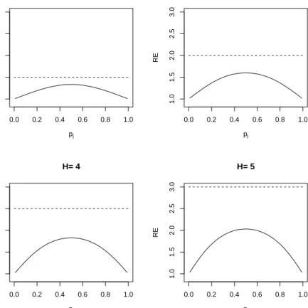
propor-tion inChen et al.(2006). In Figure 2.1, we show the relative efficiency of ˆpe

j forH = 2,3,4,

(19)

0.0 0.2 0.4 0.6 0.8 1.0 1.0 1.5 2.0 2.5 3.0 H= 2 pj RE 0.0 0.2 0.4 0.6 0.8 1.0 1.0 1.5 2.0 2.5 3.0 H= 3 pj RE 0.0 0.2 0.4 0.6 0.8 1.0 1.0 1.5 2.0 2.5 3.0 H= 4 pj RE 0.0 0.2 0.4 0.6 0.8 1.0 1.0 1.5 2.0 2.5 3.0 H= 5 pj RE

Figure 2.1. RE of ˆpe_j for H= 2,3,4, and 5.

From Figure2.1, it appears that RE is bounded by 1 and (H+ 1)/2, the same as the bounds of the RE of the mean estimator under continuous balanced RSS. The rigorous proof of this conjecture, however, is still an open question. Moreover, unlike continuous RSS , the upper bound of RE is no longer always achieved. More properties ofRE of ˆpe

j, including the

limiting behavior, the symmetry property etc, were given in Chen et al. (2006). For more details, see Chen et al. (2006).

2.2. Alternative to the EDF: Frey’s Estimator

In this section, we introduce an alternative to the EDF for discrete random variables, which incorporates tie information in an ad-hoc way. This estimator stems from an idea of

(20)

stratum CDF and the population CDF are denoted by ˆF_[F rey_r_] (x) and ˆFF rey₍_x_{), respectively.}

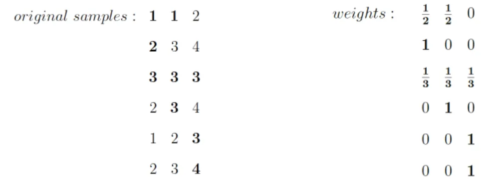
The idea is to assign equal weights to all observed tied values within each ranked set. This idea is illustrated by the following example.

Example 2.1 Suppose we have 6 sets of samples of size 3 from a discrete distribution (i.e.

H = 3, n= 2), as shown in Figure 2.2. Following the procedures in Chapter 1.2, we get the

accurately measured value (1,2,3,3,3,4) and the number of observed ties for each measured unit (including itself )(2,1,3,1,1,1). Then we assign equal weights to all units which are tied to the measured value within every set. For those units which are not measured or claimed tied to the measured units, we assign weight 0 to them. The weight for each unit is shown in Figure 2.2.

Figure 2.2. Original samples and corresponding weights

Because information about r-th order statistic is also available from the samples in which the s-th (s 6=r) order statistic is measured, due to the knowledge of ties, we have a larger

(21)

sample size than n= 2 for estimating F[r]. Frey’s method uses tie information as follows: ˆ F_[1]F rey(x) =                        0, x <1 1/2 1/2 + 1 + 1/3 = 3 11, 1≤x <2 1/2 1/2 + 1 + 1/3 + 1 1/2 + 1 + 1/3 = 9 11, 2≤x <3 1, x≥3 ˆ F_[2]F rey(x) =              0, x <1 1/2 1/2 + 1 + 1/3 = 3 11,1≤x <3 1, x≥3 ˆ F_[3]F rey(x) =              0, x < 3 1/3 + 1 1/3 + 1 + 1 = 4 7, 3≤x <4 1, x≥4. (2.2)

By using the relation F(x) = _H1 PH

r=1F[r](x), we can construct an estimate of the overall

CDF: ˆ FF rey(x) =                              0, x <1 2 11, 1≤x <2 4 11, 2≤x <3 6 7, 3≤x <4 1, x≥4. (2.3)

The estimates in (2.2) and (2.3) are equivalent to the estimates of pmf of each order stratum and the overall population, given by

(22)

ˆ f_[1]F rey(x) =                        1/2 1/2 + 1 + 1/3 = 3 11, x= 1 1 1/2 + 1 + 1/3 = 6 11, x= 2 1/3 1/2 + 1 + 1/3 = 2 11, x= 3 0, elsewhere, ˆ f_[2]F rey(x) =                1/2 1/2 + 1 + 1/3 = 3 11, x= 1 1 + 1/3 1/2 + 1 + 1/3 = 8 11, x= 3 0, elsewhere, ˆ f_[3]F rey(x) =                1/3 + 1 1/3 + 1 + 1 = 4 7, x= 3 1 1/3 + 1 + 1 = 3 7, x= 4 0, elsewhere, ˆ fF rey(x) =                              2 11, x= 1 2 11, x= 2 38 77, x= 3 1 7, x= 4 0, elsewhere. (2.4)

Now we formalize the procedure for a balanced ranked set sample. We denote a balanced ranked set sample by {(X[r]i, l[r]i, t[r]i), r = 1,· · ·, H;i = 1,· · ·, n}, where l[r]i is the number

of units which are judged to be less than the measured unit and t[r]i is the number of

units which are judged tied to the measured unit (including the measured one itself) within the ranked set from which X[r]i is selected for measurement. For example, the sample

in Example 2.1 can be written as {(1,0,2),(2,0,1),(3,0,3),(3,1,1),(3,2,1),(4,2,1)}. Let

x1 < x2 <· · · < xk denote the k distinct measured values from the ranked set sample. We

(23)

F[r], either directly because h = r, or indirectly, because X[h]i is tied with a unit having

rank r. Then Sr = {(h, i)|l[h]i < r≤l[h]i+t[h]i}, r = 1,· · ·, H. In Example 2.1, we have S1 = {(1,1),(1,2),(2,1)}, S2 = {(1,1),(2,1),(2,2)}, and S3 = {(2,1),(3,1),(3,2)}. Then

for r-th stratum, the estimator of the CDF is given by

ˆ

F_[F rey_r_] (x) = X

xj≤x

ˆ

f_[F rey_r_] (xj), (2.5)

where ˆf_[F rey_r_] (x) is the estimator of f[r](x)

ˆ f_[F rey_r_] (x) = P (h,i)∈Sr I{X_[_h_]_i=x} t[h]i P (h,i)∈Sr 1 t[h]i . (2.6)

By using the relations F(x) = _H1 PH

r=1F[r](x) and f(x) = 1

H

PH

r=1f[r](x), we can construct

the corresponding estimators for the overall population CDF and pmf. Although the esti-mators are not unbiased, they still outperform the empirical estiesti-mators in terms of mean integrated squared error (MISE), which will be shown in Chapter 2.5. One explanation was given by Liu(2016) who showed that Frey’s estimator is a modified version of Horvitz-Thompson estimator.

2.3. Nonparametric Maximum Likelihood Estimator of the CDF

Kvam and Samaniego (1994) proposed the nonparametric maximum likelihood estimator

(NPMLE) of the CDF when sample units were generated from a continuous underlying distribution. Huang (1997) proved that the NPMLE is a strongly consistent estimator of the CDF. The idea of Kvam and Samaniego (1994) can be applied in discrete cases with moderate modifications, which we will provide later.

First, we will find the likelihood function for a ranked set sample from a discrete dis-tribution, where ties of measured observations are accurately identified. Then we find the MLE of the CDF from the likelihood function. Let x1 < x2 < ... < xk denote the k distinct

(24)

values measured in the ranked set sample. For any xj, definelj, tj, vj as lj = H X r=1 nr X i=1 l[r]iI{X[r]i=xj} tj = H X r=1 nr X i=1 t[r]iI{X[r]i=xj} vj = H X r=1 nr X i=1 I{X[r]i=xj}. (2.7)

lj, tj, vj are the number of units which are judged less than, tied with, or equal to xj in

the samples (including both comparison samples and measured samples). By (A.5), the likelihood function of the ranked set sample is given by

L=

k

Y

j=1

CjFlj(xj−)(1−F(xj))sj(F(xj)−F(xj−))tj (2.8)

where F(xj−) =P(X < xj), sj =H∗vj −lj −tj, andCj is a constant.

Now we find an estimator ˆF that is restricted to the set

F ={Fˆ|Fˆ(xj−) = ˆF(xj−1), j = 2, ..., k},

and maximizes L. F excludes those estimators which assign positive probability to values which are between xj−1 and xj. Therefore (2.8) is equivalent to

L=

k

Y

j=1

CjFlj(xj−1)(1−F(xj))sj(F(xj)−F(xj−1))tj. (2.9)

For notation simplification, let φj be

φ0 =P(X < x1)

φj =F(xj),∀j = 1, ..., k

(25)

Then the log-likelihood of the ranked set sample is

`=

k

X

j=1

(logCj+ljlogφj−1+sjlog(1−φj) +tj(φj−φj−1)) (2.11)

Now, the problem is to find φ∗₀, φ∗₁, ..., φ∗_k which maximizes the log-likelihood function. The maximum likelihood estimates of φ0 and φk can be easily obtained in some special

cases. If l1 = 0, we will set ˆφ0 = 0. l1 = 0 corresponds to the situations that the smallest

valuex1 is measured as or judged tied to the first order statistic within the sets from which

they are sampled. Similarly, if sk = 0, we will set ˆφk = 1. sk = 0 corresponds to the

situations where the largest value xk are measured as or judged tied to the largest order

statistic within the sets from which they are sampled. In the following discussion, we first assume l1 6= 0 andsk6= 0.

By taking the first derivatives w.r.tφ0, φ1, ..., φk and setting those functions to 0, we have

                                                 ∂` φ0 = l1 φ0 − t1 φ1−φ0 = 0 ∂` φ1 =− s1 1−φ1 + t1 φ1−φ0 + l2 φ1 − t2 φ2−φ1 = 0 .. . ∂` φj =− sj 1−φj + tj φj−φj−1 + lj+1 φj − tj+1 φj+1−φj = 0 .. . ∂` φk−1 =− sk−1 1−φk−1 + tk−1 φk−1−φk−2 + lk φk−1 − tk φk−φk−1 = 0 ∂` φk =− sk 1−φk + tk φk−φk−1 = 0 (2.12)

Solving those equations explicitly is not practically feasible in most cases. An iterative algo-rithm was proposed by Kvam and Samaniego (1994). From the first k likelihood equations,

(26)

we have                                          φ1 =φ0+t1φ_l0 1 φ2 =φ1+t2(−₁₋s1_φ 1 + t1 φ1−φ0 + l2 φ1) −1 .. . φj+1 =φj +tj+1(− sj+1 1−φj + tj φj−φj−1 + lj+1 φj ) −1 .. . φk =φk−1+tk(− sk−1 1−φk−1 + tk−1 φk−1−φk−2 + lk φk−1) −1_. (2.13) Let H(φk, φk−1) be defined as H(φk, φk−1) =− sk 1−φk + tk φk−φk−1 .

From the last equation in (2.12), we have H(φ∗_k, φ∗_k₋₁) = 0, i.e. the maximum likelihood estimate of φk−1 andφk should satisfy H(φ∗k, φ

∗

k−1) = 0. Later, we will show that H(., .) can

be used to determine the convergence of the algorithm.

Now we prove two theorems that guarantee the existence and uniqueness of the solution, and that the computational algorithm outlined above will find that solution. Those proofs are similar to those of Kvam and Samaniego (1994), who proved similar results for their algorithm for computing the NPMLE of the CDF in the continuous cases.

Theorem 2.1 Letφ∗₀, φ∗₁, ..., φ∗_kbe the solution of the log-likelihood equations in (2.12). Then

(27)

Proof: The Hessian matrix of log-likelihood function is a tridiagonal matrix, i.e. H =                  h00 h01 h10 h11 h12 h21 . .. ... . .. ... hk−1,k hkk                  where hj,j−1 = ∂2_` ∂φj∂φj−1 = tj (φj −φj−1)2 j = 1, ..., k hjj = ∂2_` ∂φ2 j =        −l1 φ2 0 , j = 0 − sj (1−φj)2 − tj (φj−φj−1)2 − lj+1 φ2 j − tj+1 (φj+1−φj)2, j = 1, ..., k hj,j+1 = ∂2_` ∂φj∂φj+1 = tj+1 (φj+1−φj)2 , j = 0, ..., k −1 .

This matrix can be shown to be negative semidefinite. For any vector y = (y0, ..., yk+1)> ∈ Rk+1, we have y>Hy= k X j=0 hjjyj2+ k X j=1 hj,j−1yjyj−1+ k−1 X j=0 hj,j+1yjyj+1 =−l1 φ2 0 y2₀− k X j=1 ( sj (1−φj)2 +lj+1 φ2 j )y2_j − k X j=1 hj,j−1yjj2 − k X j=1 hj,j+1yjj2 + k X j=1 hj,j−1yjyj−1+ k−1 X j=0 hj,j+1yjyj+1 =−l1 φ2 0 y2₀− k X j=1 ( sj (1−φj)2 +lj+1 φ2 j )y2_j − k X j=1 hj,j−1(yj −yj−1)2 ≤0.

(28)

y>Hy equals to 0 if and only if y = 0. The fact that the Hessian matrix is negative semidefinite implies that the log-likelihood function is concave. Therefore, the unique max-imum exists.

Theorem 2.2 Let φ∗₀, φ∗₁, ..., φ∗_k denote the MLE. The estimates φˆj, j = 1, ..., k constructed

from any initial value φˆ0 have the following properties: 1) If φˆ0 < φ∗0, then φˆj < φ∗j and H( ˆφk,φˆk−1)>0. 2)If φˆ0 > φ∗0, then φˆj > φ∗j and H( ˆφk,φˆk−1)<0.

Proof: Givent1 >0 andl1 >0, the first equation in (2.13) implies thatφ1 is an increasing

function inφ0. Therefore, ˆφ1 < φ∗1 if ˆφ0 < φ∗0. Also from the first equation in (2.13), we have

that φ1 −φ0 =t1φ_l₁0 is an increasing function in φ0, which implies that ˆφ1−φˆ0 < φ∗1−φ

∗

0.

Assume ˆφj < φ∗j and ˆφj−φˆj−1 < φ∗j −φ∗j−1. From (j+ 1)th equation in (2.13), we have

that φj+1 and φj+1 −φj are increasing functions in φj and φj −φj−1. Thus ˆφj+1 < φ∗j+1

and ˆφj+1 −φˆj < φ∗j+1 −φ

∗

j. By induction, we have ˆφj < φ∗j for all j = 1, ..., k. Moreover, H(φk, φk−1) is a decreasing function in φk and φk−φk−1, which implies thatH( ˆφk,φˆk−1)>

H(φ∗_k, φ∗_k₋₁) = 0. Similarly, we can prove the other direction.

With Theorem 2.2, we can apply a binary search algorithm to find ˆφ∗_j, j = 0,· · ·, k. For any measured valuexj, the estimated probability is computed as

ˆ

p_jN P M LE = ˆφ∗_j −φˆ∗_j₋₁, j = 1, ..., k.

2.4. Resampling Methods for Ranked Set Sampling

Due to the complexity of the sampling procedure, resampling techniques are often used for variance estimation for estimators made from ranked set samples. Because bootstrap methods are based on sampling from an estimated CDF, we now have several options for implementation of a RSS bootstrap. In this section, we outline several methods available for a RSS bootstrap with our new CDF’s.

(29)

Modarres et al. (2006) summarized three bootstrap methods for continuous RSS: boot-strap RSS by rows (BRSSR), bootstrap RSS (BRSS), and mixed row bootstrap RSS

(M RBRSS) in the context of balanced continuous RSS. The idea of BRSSR is to

con-sider each order stratum separately. For each stratum, we assign equal probability to each row and resample with replacement to generate a sample of the same size. In the context of continuous RSS,BRSSRis equivalent to estimating the EDF of each stratum separately. Let

ˆ

F_[e_r_] denote the EDF of r-th order stratum, where ˆF_[e_r_](x) = _n1 Pn

i=1I{X[r]i≤x}, r = 1,· · ·, H.

Then generaten units from ˆFe

[r]forr= 1,· · ·, H and combine the samples generated to form

a bootstrap sample. One drawback of this method is that it doesn’t work for n= 1.

The second approach BRSS provides an alternative that also works for the single cycle RSS. Instead of estimating the CDF of each stratum separately, BRSS obtains the EDF ˆF

of the overall population first. Then bootstrap RSS is simulated from ˆF by using procedures in section (1.2) with the same H and n that was used in the original design.

BRSSR and BRSS, however, don’t use the partial ordering information in the ranked

set sample, i.e. the units inr-th stratum have a higher probability of being less than the units in s-th stratum than being greater than the units in s-th stratum for r < s. Based on this concern, Modarres et al. (2006) proposed another method, called M RBRSS. M RBRSS

is different with BRSS only in generating the original samples. Instead of drawing H

units from ˆFe in the first step in (1.2), M RBRSS draws H units by choosing one unit independently from each ˆFe

[r] and then ranks them to get the measured unit. Because this

method generates samples from ˆFe

r, it doesn’t work for n= 1 either.

Although all three methods are discussed in the context of balanced RSS with continuous underlying distribution in Modarres et al. (2006), they can be easily extended to discrete RSS or unbalanced RSS. But none of the methods uses information about ties. Therefore we explore how to incorporate tie information into the bootstrap procedure.

An intuitive way to use tie information is to treat ˆFf rey _{or ˆ}_FN P M LE _{as the parent}

(30)

estimated CDF. In the following discussion, we call the new methodsBRSSF andBRSSM, respectively.

One potential problem of BRSSM is to deal with the categories x < x1 and x > xk.

One possible solution is that we can artificially create two possible categories ˆx0 and ˆxk+1.

There are many possible choices of ˆx0 and ˆxk+1. For example, an ad-hoc approach is to

set ˆx0 = x1 and ˆxk+1 = xk. The potential result of using this combination is that it will

artificially increase the probability of samplingx1 andxk and therefore the observed number

of units tied tox1 orxk. So our suggestion is to use a second choice: that is ˆx0 =x1−δ and

ˆ

xk+1 =xk+δ, where δ is the smallest increment observed from {x1,· · ·, xk}.

Suppose the parameter of interest is T(F). Then the general bootstrap procedure for estimating the standard error of the estimator T( ˆF) is summarized as follows:

1. Obtain the estimate ˆT from the original sample {X[r]i, l[r]i, t[r]i}.

2. Generate B (eg. B = 50, or 100) bootstrap ranked set samples {X_[(_rb_])_i, l(_[_rb_])_i, t(_[_rb_])_i}, b = 1,· · ·, B by using any bootstrap method.

3. Compute ˆT(b) _{from each bootstrap sample.}

4. Then the standard error of T( ˆF) can be estimated as

ˆ SE = r 1 B −1( ˆT (b)₎₋_T¯ˆ₎2_, where T¯ˆ= 1 B PB b=1Tˆ (b)_.

By using the estimated standard error, we can construct the 95%(α = 5%) confidence interval

( ˆT −z(1−α/2)SE,ˆ Tˆ+z(1−α/2)SEˆ ).

An alternative approach to z-confidence interval is to use the empirical confidence interval. The resulting confidence interval is ( ˆT(α/2),Tˆ(1−α/2)), where ˆT(α/2) and ˆT(1−α/2)denote theα/2

and 1−α/2 percentile of ˆT(b), b= 1,· · ·, B. To obtain a more accurate empirical confidence interval, a relatively largeB (1000 or more) is required.

(31)

The resampling procedures can be used to make inference on statistical quantities. In Section 3.4.3, we will apply these bootstrap methods to make inference on the population mean. In Section 4.3.2, we will apply these bootstrap methods to make inference on the population variance.

2.5. Simulation Study

In this section, we conduct a simulation study to compare the performance of the EDF, Frey’s estimator, and the NPMLE for some common discrete distributions. The performance of a CDF estimator is evaluated in terms of mean integrated squared error (MISE). MISE of an estimator ˆF is computed as the sum of mean square errors over all support points, i.e.

M ISE( ˆF) = EX

x∈S

(f(x)−fˆ(x))2 =X

x∈S

M SE( ˆf(x)). (2.14)

Let ˆFSRS denote the EDF of F from a simple random sample having the same number of measured units as the ranked set sample. Then the relative efficiency of an estimator ˆF is defined as the ratio of MISE of ˆF to MISE of ˆFSRS_{, i.e.}

RE( ˆF) = M ISE( ˆF

SRS₎

M ISE( ˆF) .

In our simulation, RE is estimated by 10000 replications.

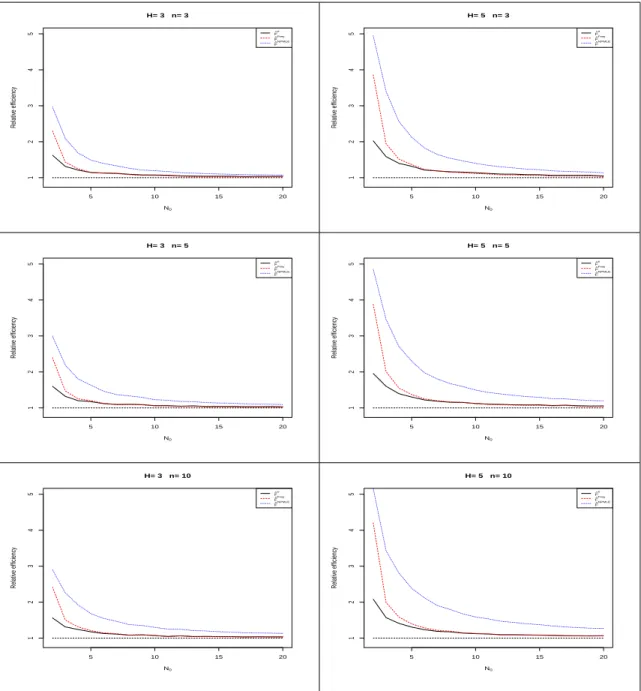
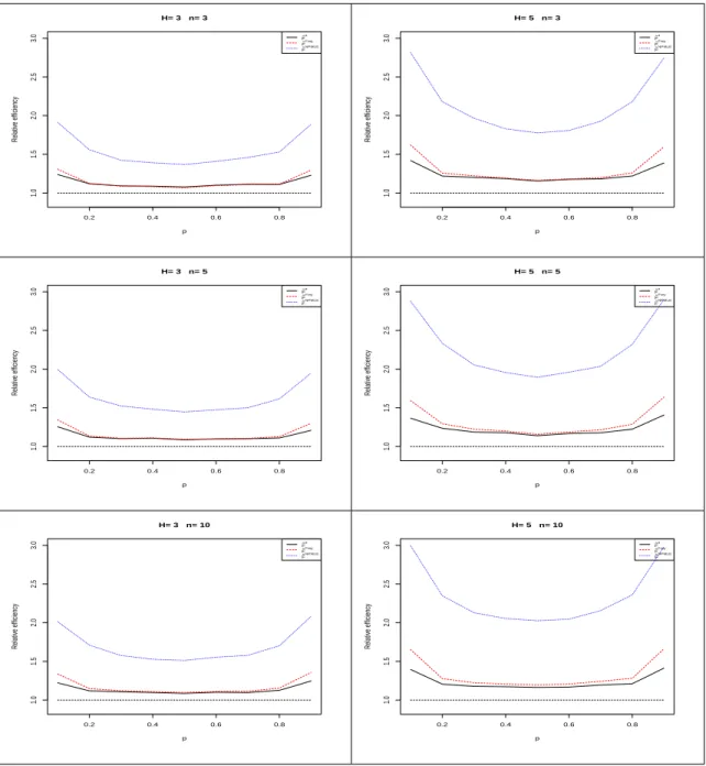
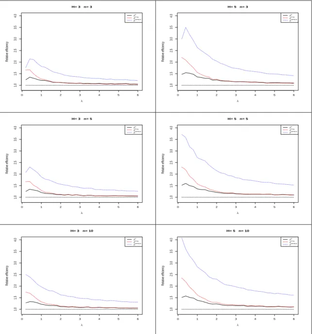
Figures2.3,2.4and2.5exhibit the simulated relative efficiency of ˆFe, ˆFF rey, and ˆFN P M LE

for set sizes H = 3,5 and cycle size n = 3,5,10. The distributions used in generating the sample include Discrete uniform distribution (N), Binomial distribution(10, p) and Poisson distribution (λ). When constructing those three estimators, we don’t use any information about the sample generation distribution.

From Figures 2.3, 2.4 and 2.5, ˆFN P M LE _{always has the highest RE, which suggests}

ˆ

FN P M LE is the most efficient estimator in terms of MISE. Moreover, ˆFF rey is more efficient

(32)

greater than 1, which imply that they are more efficient than the SRS estimator for the balanced ranked set sample.

5 10 15 20 1 2 3 4 5 H= 3 n= 3 N0 Relativ e efficiency F ê F ^Frey F ^NPMLE 5 10 15 20 1 2 3 4 5 H= 5 n= 3 N0 Relativ e efficiency F ê F ^Frey F ^NPMLE 5 10 15 20 1 2 3 4 5 H= 3 n= 5 N0 Relativ e efficiency F ê F ^Frey F ^NPMLE 5 10 15 20 1 2 3 4 5 H= 5 n= 5 N0 Relativ e efficiency F ê F ^Frey F ^NPMLE 5 10 15 20 1 2 3 4 5 H= 3 n= 10 N0 Relativ e efficiency F ê F ^Frey F ^NPMLE 5 10 15 20 1 2 3 4 5 H= 5 n= 10 N0 Relativ e efficiency F ê F ^Frey F ^NPMLE

(33)

0.2 0.4 0.6 0.8 1.0 1.5 2.0 2.5 3.0 H= 3 n= 3 p Relativ e efficiency F ê F ^Frey F ^NPMLE 0.2 0.4 0.6 0.8 1.0 1.5 2.0 2.5 3.0 H= 5 n= 3 p Relativ e efficiency F ê F ^Frey F ^NPMLE 0.2 0.4 0.6 0.8 1.0 1.5 2.0 2.5 3.0 H= 3 n= 5 p Relativ e efficiency F ê F ^Frey F ^NPMLE 0.2 0.4 0.6 0.8 1.0 1.5 2.0 2.5 3.0 H= 5 n= 5 p Relativ e efficiency F ê F ^Frey F ^NPMLE 0.2 0.4 0.6 0.8 1.0 1.5 2.0 2.5 3.0 H= 3 n= 10 p Relativ e efficiency F ê F ^Frey F ^NPMLE 0.2 0.4 0.6 0.8 1.0 1.5 2.0 2.5 3.0 H= 5 n= 10 p Relativ e efficiency F ê F ^Frey F ^NPMLE

(34)

0 1 2 3 4 5 6 1.0 1.5 2.0 2.5 3.0 3.5 4.0 H= 3 n= 3 λ Relativ e efficiency F ê F ^Frey F ^NPMLE 0 1 2 3 4 5 6 1.0 1.5 2.0 2.5 3.0 3.5 4.0 H= 5 n= 3 λ Relativ e efficiency F ê F ^Frey F ^NPMLE 0 1 2 3 4 5 6 1.0 1.5 2.0 2.5 3.0 3.5 4.0 H= 3 n= 5 λ Relativ e efficiency F ê F ^Frey F ^NPMLE 0 1 2 3 4 5 6 1.0 1.5 2.0 2.5 3.0 3.5 4.0 H= 5 n= 5 λ Relativ e efficiency F ê F ^Frey F ^NPMLE 0 1 2 3 4 5 6 1.0 1.5 2.0 2.5 3.0 3.5 4.0 H= 3 n= 10 λ Relativ e efficiency F ê F ^Frey F ^NPMLE 0 1 2 3 4 5 6 1.0 1.5 2.0 2.5 3.0 3.5 4.0 H= 5 n= 10 λ Relativ e efficiency F ê F ^Frey F ^NPMLE

(35)

2.6. Conclusion

In this section, we proposed two new estimators of the CDF and pmf under discrete RSS. Frey’s Estimator assigns equal weights to all tied values within each ranked set and the weighted CDF is computed within each order stratum. It has been shown to be a more efficient estimator compared to the EDF via simulation studies. The NPMLE was proposed by incorporating information into the likelihood function. Then the optimal solution can be found via a numerical method. By simulation studies, it showed a significant improvement over the other two estimators in terms of MISE. Moreover, another advantage of the NPMLE is that it can be easily adapted to the unbalanced case.

However, there are still some limitations of the new estimators. First, Frey’s estimator doesn’t work well for unbalanced cases. Moreover, from the simulation studies, Frey’s esti-mator only have slight improvements over the EDF under a lot of settings. Although the NPMLE improved the RE significantly, it required the assumption that the probabilities can be only assigned to those observed values. How to relax this assumption needs further investigations.

(36)

CHAPTER 3

ON ESTIMATING THE POPULATION MEAN

3.1. Background

Estimating the population mean is one of the most studied topics in RSS research. Sup-pose the mean, variance, cumulative distribution function, and probability mass function of the underlying population areµ, σ2_, _F₍_x_{), and}_f₍_x_{) and the corresponding mean, variance,}

cumulative distribution function, and probability mass function of r-th order stratum are

µ[r], σ2_[_r_],F[r](x), andf[r](x). Let{(X[r]i, l[r]i, t[r]i);r= 1, ..., H;i= 1, ..., n}denote a balanced

discrete ranked set sample, wherel[r]iandt[r]i are the number of units which are judged to be

less than the measured unit and the number of units which are judged tied to the measured unit (including the measured one itself) within the set from which X[r]i is selected. Then

the regular RSS mean estimator is

ˆ µRSS = 1 H H X r=1 ˆ µRSS_[_r_] = 1 H H X r=1 (1 n n X i=1 X[r]i), where ˆµRSS

[r] is the estimator of r-th stratum mean.

It is simple to verify that ˆµRSS _{is an unbiased estimator of the population mean} _µ_{. To}

compare the efficiency of ˆµRSS over the SRS estimator ˆµSRS from a simple random sample with the same size as the ranked set sample, we define the relative efficiency of any mean estimator ˆµ as

RE(ˆµ) = M SE(ˆµ

SRS₎

M SE(ˆµ) , (3.1) where M SE(ˆµSRS_{) and} _{M SE}_(ˆ_µ_{) are mean square errors of SRS estimator ˆ}_µSRS _{and ˆ}_µ_,

(37)

to RE(ˆµRSS) = σ 2 1 H PH r=1σ[2r] , (3.2)

The RE of ˆµRSS _{for continuous balanced cases was proved to be bounded by 1 and (}_H_{+ 1)}_/₂

inTakahasi and Wakimoto (1968).

Table 3.1 exhibits the RE’s of ˆµRSS for some common discrete underlying distributions whenH = 2,3,4,5. The relative efficiency is still bounded by 1 and (H+ 1)/2 for the distri-butions shown in the Table3.1. Whether this upper bound holds for all discrete distributions has not been determined.

Table 3.1. Relative Efficiency of ˆµRSS from a balanced discrete ranked-set sample for some common discrete distributions

Distribution Parameter H = 2 H= 3 H = 4 H = 5 Uniform (N0) 3 1.421 1.801 2.146 2.466 4 1.455 1.880 2.287 2.671 5 1.471 1.920 2.359 2.780 10 1.483 1.980 2.463 2.941 20 1.498 1.995 2.491 2.985 Bin(10, p) .1 1.387 1.734 2.049 2.339 .3 1.444 1.857 2.246 2.615 .5 1.450 1.872 2.271 2.652 .7 1.444 1.857 2.246 2.615 .9 1.387 1.734 2.049 2.339 Poisson 1 1.378 1.718 2.029 2.316 2 1.424 1.815 2.181 2.527 5 1.450 1.874 2.278 2.669 10 1.437 1.839 2.214 2.567

An interesting fact observed from Table 3.1 is that the relative efficiency of ˆµRSS ap-proaches the upper bound (H + 1)/2 as the parameter of discrete uniform distribution

(38)

is close to the continuous uniform distribution which has been shown to have the relative efficiency of (H+ 1)/2.

3.2. Frey’s Estimator of the Population Mean

Note that ˆµRSS _{doesn’t use any tie information.} _Frey ₍₂₀₁₂_{) proposed an estimator,}

denoted by ˆµF rey_{, which incorporates the tie information in the context of continuous JPS.}

The same idea can be applied in discrete RSS. This estimator only works for the balanced discrete RSS.

Suppose we have a balanced ranked set sample{(X[r]i, l[r]i, t[r]i), r = 1,· · ·, H;i= 1,· · ·n}.

Let x1 < x2 < · · · < xk denote k distinct measured values. Define the index set Sr =

{(h, i)|l[h]i < r≤l[h]i+t[h]i}. Then ˆµF rey is ˆ µF rey = 1 H H X r=1 ˆ µF rey_[_r_] , (3.3)

where ˆµF rey_[_r_] is the estimate of the mean of r-th stratum

ˆ µF rey_[_r_] = P (h,i)∈Sr X[h]i t[h]i P (h,i)∈Sr 1 t[h]i . (3.4)

Frey(2012) showed via simulation studies that ˆµF rey _{is more efficient than the regular mean}

estimator ˆµRSS in the context of continuous JPS.

Liu (2016) proposed a modified Horvitz-Thompson estimator ˆµHT _{for discrete RSS. Let} π[r]i be the inclusion probability of X[r]i, which is

π[r]i = t[r]i

H

for balanced cases. For the unbalanced cases, π[r]i =

P h

P

(h,i)∈Srnr

N , where nr is the number

of units selected from the r-th ranked class. Let ˆµHT _{and ˆ}_µHT

(39)

Horvitz-Thompson estimator of the population mean and r-th stratum mean, where ˆ µHT = 1 H H X r=1 ˆ µHT_[_r_] (3.5) and ˆ µHT_[_r_] = P (h,i)∈Sr X[h]i π[h]i P (h,i)∈Sr 1 π[h]i . (3.6)

They showed that their estimator was equivalent to ˆµF rey _{under balanced discrete RSS,}

which explained why Frey’s estimator performed so well in balanced discrete cases.

3.3. Nonparametric Maximum Likelihood Estimator of µ

In this section, we propose a new plug-in estimator of the mean ˆµN P M LE _{by using the}

nonparametric maximum likelihood estimator (NPMLE) of the CDF. It is well-known that

µis a functional of the CDF F for discrete distributions, i.e.

µ=T(F) = X

x∈S

x(F(x)−F(x−)),

where S is the support of the distribution. Many estimators can be constructed using this relationship. For example, ˆµRSS is the plug-in estimator by using ˆFe, i.e. ˆµRSS = T( ˆFe),

and ˆµF rey _{is the plug-in estimator by using ˆ}_FF rey_{, i.e. ˆ}_µF rey ₌_T_{( ˆ}_FF rey₎_.

Now let us construct ˆµN P M LE _{by using ˆ}_FN P M LE_{. Let}_x

1 <· · ·< xk denote thekdistinct

measured values in the ranked set sample. ˆµN P M LE is defined as

ˆ µN P M LE =T( ˆFN P M LE) = ˆx0φˆ0+ k X j=1 xj( ˆφj−φˆj−1) + ˆxk+1(1−φˆk) (3.7)

where ˆφ0,· · ·,φˆk is the approximation of the NPMLE of the CDF from section (2.3), ˆx0 is an

estimate of values which are less thanx1, and ˆxk+1 is an estimate of values which are greater

than xk. Similar to 2.4, there are many choices of ˆx0 and ˆxk+1. For example, one reasonable

(40)

ˆ

xk+1 =xk+δ, whereδis the smallest increment observed from{x1,· · ·, xk}. In the following

discussion, we will always use ˆx0 =x1 and ˆxk+1 =xk to construct ˆµN P M LE.

3.4. Simulation Study

In this section, we examine the performance of the proposed estimators via simulation studies. There are three simulation studies in this section: Section 3.4.1 is to compare the performance of those estimators for balanced discrete RSS; Section 3.4.2 is to show the performance of ˆµN P M LE _{for unbalanced RSS; Section} _3.4.3 _{is to examine whether the}

bootstrap method proposed in Section 2.4 can be used for accurate inference on the mean. In all simulations, when computing ˆµN P M LE, we use that ˆx0 = x1 and ˆxk+1 = xk in (3.7).

For the bootstrap procedure from ˆFN P M LE_{, we increase ˆ}_φ

1 by ˆφ0 and also increase ˆφk by

ˆ

φk+1.

3.4.1. Performance of Estimators Under Balanced Discrete Ranked Set Sampling

This simulation is designed to compare those estimators under balanced discrete RSS in terms of relative efficiency (RE). Let ˆµSRS be the mean estimator from a simple random sample which has the same sample size as the ranked set sample. The RE of an estimator ˆµ

is defined as the ratio of the mean square error (MSE) of ˆµSRS _{to that of ˆ}_µ_{, i.e.}

RE(ˆµ) = M SE(ˆµ

SRS₎

M SE(ˆµ) . (3.8)

In our simulation studies, M SE(ˆµ) is estimated based on 10000 simulated samples for each combinations of parameters.

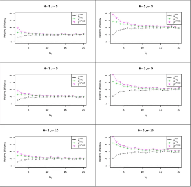
We set the set size (H) as 3 and 5. The cycle size (n) is set to be 3, 5, and 10. For the underlying distribution, we choose three common discrete distributions, including Discrete Uniform distribution ( Uniform (N0)), Poisson distribution (P oi(λ)), and binomial

(41)

for each distribution. The results for the three distributions are shown in Figures 3.1, 3.2, and 3.3, respectively. 5 10 15 20 1 2 3 4 5 H= 3 ,n= 3 N0 Relativ e Efficiency ● ● ● ● ● ● ● ● ● ● ● ● ● ● ● ● ● ● ● ● _µ^RSS µ^Frey µ^NPMLE 5 10 15 20 1 2 3 4 5 H= 5 ,n= 3 N0 Relativ e Efficiency ● ● ● ● ● ● ● ● ● ● ● ● ● ● ● _● ● _● ● ● _µ^RSS µ^Frey µ^NPMLE 5 10 15 20 1 2 3 4 5 H= 3 ,n= 5 N0 Relativ e Efficiency ● ● ● ● ● ● ● ● ● ● ● ● ● ● ● ● ● ● ● ● _µ^RSS µ^Frey µ^NPMLE 5 10 15 20 1 2 3 4 5 H= 5 ,n= 5 N0 Relativ e Efficiency ● ● ● ● ● ● ● ● ● ● ● ● ● _● ● ● ● ● ● ● _µ^RSS µ^Frey µ^NPMLE 5 10 15 20 1 2 3 4 5 H= 3 ,n= 10 N0 Relativ e Efficiency ● ● ● ● ● ● ● ● ● ● ● ● ● ● ● ● ● ● ● ● _µ^RSS µ^Frey µ^NPMLE 5 10 15 20 1 2 3 4 5 H= 5 ,n= 10 N0 Relativ e Efficiency ● ● ● ● ● ● ● ● ● ● ● ● ● ● ● ● ● ● ● ● _µ^RSS µ^Frey µ^NPMLE

(42)

0.2 0.4 0.6 0.8 1 2 3 4 5 H= 3 ,n= 3 p Relativ e Efficiency ● ● ● ● ● ● ● ● ● ● ● ● ● ● ● ● ● _● ● ● _µ^RSS µ^Frey µ^NPMLE 0.2 0.4 0.6 0.8 1 2 3 4 5 H= 5 ,n= 3 p Relativ e Efficiency ● ● ● ● ● ● ● ● ● ● ● ● ● ● ● ● ● ● ● ● _µ^RSS µ^Frey µ^NPMLE 0.2 0.4 0.6 0.8 1 2 3 4 5 H= 3 ,n= 5 p Relativ e Efficiency ● ● ● ● ● ● ● ● ● ● ● ● ● ● ● ● _● _● ● ● _µ^RSS µ^Frey µ^NPMLE 0.2 0.4 0.6 0.8 1 2 3 4 5 H= 5 ,n= 5 p Relativ e Efficiency ● ● ● ● ● ● ● ● ● ● ● ● ● ● ● ● _● ● ● ● _µ^RSS µ^Frey µ^NPMLE 0.2 0.4 0.6 0.8 1 2 3 4 5 H= 3 ,n= 10 p Relativ e Efficiency ● ● ● ● ● ● ● ● ● ● ● ● _● ● ● ● ● ● ● ● _µ^RSS µ^Frey µ^NPMLE 0.2 0.4 0.6 0.8 1 2 3 4 5 H= 5 ,n= 10 p Relativ e Efficiency ● ● ● ● ● ● ● ● ● ● ● ● ● ● ● ● ● ● ● ● _µ^RSS µ^Frey µ^NPMLE

(43)

2 4 6 8 10 1 2 3 4 5 H= 3 ,n= 3 λ Relativ e Efficiency ● ● ● ● ● ● ● ● ● ● ● ● ● ● ● ● ● ● ● ● ● _µ^RSS µ^Frey µ^NPMLE 2 4 6 8 10 1 2 3 4 5 H= 5 ,n= 3 λ Relativ e Efficiency ● ● ● ● ● ● ● ● ● ● ● ● ● ● ● ● ● ● ● ● ● _µ^RSS µ^Frey µ^NPMLE 2 4 6 8 10 1 2 3 4 5 H= 3 ,n= 5 λ Relativ e Efficiency ● ● ● ● ● ● ● ● ● ● ● ● ● ● ● ● _● _● ● ● ● _µ^RSS µ^Frey µ^NPMLE 2 4 6 8 10 1 2 3 4 5 H= 5 ,n= 5 λ Relativ e Efficiency ● ● ● ● ● ● ● ● ● ● ● ● ● ● ● ● ● ● ● ● ● _µ^RSS µ^Frey µ^NPMLE 2 4 6 8 10 1 2 3 4 5 H= 3 ,n= 10 λ Relativ e Efficiency ● ● ● ● ● ● ● ● ● ● ● ● ● ● ● ● ● ● ● ● ● _µ^RSS µ^Frey µ^NPMLE 2 4 6 8 10 1 2 3 4 5 H= 5 ,n= 10 λ Relativ e Efficiency ● ● ● ● ● ● ● ● ● ● ● ● ● ● ● ● ● ● ● ● ● _µ^RSS µ^Frey µ^NPMLE

(44)

From Figures 3.1,3.2, and3.3, we see that the RE’s of all RSS estimators are uniformly greater than 1 for all underlying distributions, which implies that those mean estimators are more efficient than SRS estimator with the same number of measured units. Also, the relative efficiency of ˆµRSS is still bounded by H+1₂ , which is consistent with the conclusion

under continuous RSS. But for ˆµF rey and ˆµN P M LE, the maximum relative efficiency may

exceed H₂+1 as a result of using the information about ties. Moreover, ˆµF rey outperforms

ˆ

µRSS, which is consistent with the conclusion for continuous cases in Frey (2012). ˆµN P M LE

outperforms ˆµRSS and ˆµF rey in every case. In other words, the proposed estimator is the

most efficient estimator among those three estimators for the distributions considered.

3.4.2. Performance of Estimators Under Unbalanced Discrete Ranked Set Sampling

The RE of a mean estimator with an unbalanced ranked set sample is affected by many factors, including the sampling proportion from each stratum, underlying distribution, etc. To examine the effect of unbalance, we chose a simulation setting of H = 2 and N = 30. The sample size from the first ranked stratum varies from 1 to 29. Then to study the effect of varying distributions, we simulated these unbalanced ranked set samples from six distributions: discrete uniform(N0 = 5,10), Poisson(λ = 1,3) and binomial(n = 10, p =

.2, .5). Each setting of distribution and sample allocation was replicated 10000 times, and the four estimators of mean ˆµRSS_,_µ_ˆF rey_,_µ_ˆHT_, _{and ˆ}_µN P M LE _{computed from each. Then the}

empirical bias, variance, MSE, and RE of each estimator were computed from the replicates. Figure3.4 shows the RE as a function of the sampling proportion from 1-st ranking class for each distribution. Table 3.2 showed the simulated bias, variance and MSE of each mean estimator for binomial(10,0.2).

(45)

0.0 0.2 0.4 0.6 0.8 1.0 0.5 1.0 1.5 2.0 2.5 3.0 Discrete(5) N=30

sampling proportion from 1st stratum

RE ● ● ●● ● ●● ●● ● ●● ● ● ● ● ● ● ●● ●_● ● ● ● ● ● ● ● ● _µ^RSS µ^Frey µ^NPMLE µ^HT 0.0 0.2 0.4 0.6 0.8 1.0 0.5 1.0 1.5 2.0 2.5 3.0 Discrete(10) N=30

RE ● ● ● ●● ●● ●● ● ● ● ●● ● ● ● ● ●●_● ● ●_● ● ● ● ● ● ● _µ^RSS µ ^Frey µ ^NPMLE µ ^HT 0.0 0.2 0.4 0.6 0.8 1.0 0.5 1.0 1.5 2.0 2.5 3.0 Poisson(1) N=30

RE ● ● ● ●● ●● ● ● ●●●● ● ●_{● ●} ●●_● ● ●_● ● ● ● ● ● ● ● _µ^RSS µ^Frey µ^NPMLE µ^HT 0.0 0.2 0.4 0.6 0.8 1.0 0.5 1.0 1.5 2.0 2.5 3.0 Poisson(3) N=30

RE ● ● ● ●● ●● ●● ●●● ● ● ● ●● ●●_● ● ●_● ● ● ● ● ● ● ● _µ^RSS µ ^Frey µ ^NPMLE µ ^HT 0.0 0.2 0.4 0.6 0.8 1.0 0.5 1.0 1.5 2.0 2.5 3.0 Binomial(10,0.2) N=30

RE ● ● ● ●● ●● ●● ● ●● ● ● ● ●_{● ●} ●_● ●_● ● ● ● ● ● ● ● ● _µ^RSS µ^Frey µ^NPMLE µ^HT 0.0 0.2 0.4 0.6 0.8 1.0 0.5 1.0 1.5 2.0 2.5 3.0 Binomial(10,0.5) N=30

RE ● ● ● ●● ●● ●● ● ●● ● ● ● ● ● ●● ●_● ● ● ● ● ● ● ● ● ● _µ^RSS µ ^Frey µ ^NPMLE µ ^HT

Figure 3.4. Relative efficiency of mean estimators versus sampling proportion from 1st order stratum fordiscrete uniform(N0 = 5,10), Poisson(λ= 1,3) and binomial(n = 10,p =.2, .5)

(46)

From Figure 3.4, ˆµN P M LE _{is the most efficient estimator compared to ˆ}_µRSS_{, ˆ}_µF rey_{, and}

ˆ

µHT _{for all distributions considered. It always outperforms the SRS estimator as the RE}

is always greater than 1. Also, the maximum RE of ˆµN P M LE is not always achieved when sampling proportion from 1st stratum is 0.5, which suggests that ˆµN P M LE _{for unbalanced}

RSS may have a higher RE than ˆµN P M LE _{for balanced RSS as would be expected, based on}

the theory of Neyman allocation.

But ˆµF rey, ˆµHT, and ˆµRSSmay not always outperform the SRS estimator, especially when the proportion is close to 0 or 1. Moreover, ˆµF rey _{and ˆ}_µHT _{are more efficient than ˆ}_µRSS_.

ˆ

µF rey and ˆµHT have similar MSE’s and they have exactly the same RE’s when sampling

proportion p = .5 because they are equivalent when p = .5. Although MSE’s of ˆµF rey

and ˆµHT _{are similar for all the sampling proportions, the source of the components of the}

MSE are different. As shown in Table 3.2, ˆµF rey may have a serious bias when sampling proportion is close to 0 or 1, whereas the bias of ˆµHT is always small. In other words, ˆµHT

has a relatively high variance compared to ˆµF rey _{when the sampling proportion is close to 0}

or 1 because ˆµHT _{correctly differentially weights the observations from the two strata based}

(47)

Table 3.2. Simulated bias, variance and MSE of mean estimators for Binomial (10, 0.2) based on 10000 replicates (N = 30)

ˆ

µF rey µˆHT µˆN P M LE

Proportion Bias Variance MSE Bias Variance MSE Bias Variance MSE

0.1 0.164 0.044 0.071 0.001 0.069 0.069 0.020 0.034 0.035 0.2 0.103 0.038 0.048 0.002 0.043 0.043 0.008 0.033 0.033 0.3 0.062 0.033 0.038 0.001 0.035 0.035 0.003 0.032 0.032 0.4 0.026 0.032 0.033 -0.004 0.032 0.032 -0.004 0.032 0.032 0.5 0.000 0.033 0.033 0.000 0.033 0.033 -0.001 0.033 0.033 0.6 -0.032 0.035 0.036 0.000 0.035 0.035 -0.002 0.033 0.033 0.7 -0.073 0.038 0.043 -0.002 0.041 0.041 -0.007 0.035 0.035 0.8 -0.130 0.043 0.060 -0.004 0.053 0.053 -0.014 0.036 0.036 0.9 0.226 0.053 0.104 -0.010 0.097 0.097 -0.033 0.041 0.042

3.4.3. Inference on Population Mean

We conducted a simulation study designed to examine whether the bootstrap method proposed in Section 2.4 can be used for accurate inference on the mean. Specifically, we examine the performance of the bootstrap based estimator of standard error and the coverage probability of the confidence interval procedures produced from that estimator, as outlined in Section 2.4.

The simulation was conducted as a factorial experiment with three factors: distribution, set size, and cycle size. Samples were simulated from six underlying distributions: discrete uniform(5), discrete uniform(10), binomial(10, 0.2), binomial(10,.5), Poisson(1), and Pois-son(5). From each distribution, we generated R = 2000 balanced ranked set samples. We examined two settings of set size and three settings of number of cycles: H = 3 and 5, and

n= 3, 5, and 10.

From each sample, we computed ˆµN P M LE and its standard error using the BRSSM

(48)

bootstrap ranked set samples with the same ranked set sample design as its parent sample. From each sample, we computed ˆµ(b)N P M LE _for _b _{= 1}_,_{· · ·}_,_{100. Then the standard error of}

ˆ µN P M LE was estimated by ˆ SE(ˆµN P M LE) = v u u t 1 B −1 B X b=1 {µˆ(b)N P M LE₋_µ¯_ˆN P M LE_}2_, _(3.9) where ¯ ˆ µN P M LE = 1 B B X b=1 ˆ µ(b)N P M LE.

For each of the samples, a 95% confidence interval forµ was also constructed as follows:

(ˆµN P M LE−z0.975∗SE,ˆ µˆN P M LE+z0.975∗SEˆ ). (3.10)

To evaluate the results of the simulation, we computed the empirical bias of the standard error estimator (3.9) and the coverage probability of the confidence intervals (3.10). To examine the bias of ˆSE(ˆµN P M LE_{), we first computed the average of ˆ}_SE_(ˆ_µN P M LE_{) for the} R= 2000 replicates for each simulating setting which we denote by SE¯ˆ (ˆµN P M LE). Then we compared this average to the simulated standard error of ˆµN P M LE_{, denoted by}_SE∗_. _SE∗ _is

simply the sample standard deviation of theR = 2000 replicates of ˆµN P M LE_{. To investigate}

the performance of the confidence intervals, we computed the proportion of intervals which cover the mean of the relevant parent distribution.

The results of this evaluation are shown in Table3.3. For each of the scenarios considered, we display SE¯ˆ , SE∗, and the confidence interval coverage proportion. These are shown in columnsSE¯ˆ , SE∗, and Coverage of the table.

We first note that the standard errors and their estimates do behave as we would expect based on the theory of ranked set sampling. They decrease with increasing sample size, and they show the effect of greater precision as H increases. For example, we observe that SE¯ˆ

and SE∗ are both smaller for the cases of H = 5, n = 3 than for H = 3, n = 5, as theory would predict.

(49)

To examine the performance of the bootstrap procedure for inference, notice that the standard error estimator appears to have small bias. That is, SE¯ˆ and SE∗ are usually quite close to each other. The most noticeable bias occurs for the binomial and Poisson distributions, where the biases are all negative, and most noticeable for small sample sizes. The reason for this could be that a support point at the endpoint of the support range is less likely to be observed in a small sample, resulting in an underestimate of the standard error. The binomial and Poisson distributions do have relatively smaller probability masses near the edges of their range.

Turning to the confidence intervals, we see that for all scenarios, the coverage probabilities are close to their nominal level of 95%. The slight undercoverage of confidence intervals for the Binomial and Poisson distributions, especially for small sample size, is presumably due to the small negative bias of the estimators of the standard errors.

(50)

Table 3.3. Coverage probability, the average of estimates of the standard error of ˆµN P M LE_,

and the simulated standard error of ˆµN P M LE _{based on 2000 replicates}

H = 3 H= 5

Distribution n SE¯ˆ SE∗ Coverage SE¯ˆ SE∗ Coverage

uniform (5) 3 0.064 0.063 0.928 0.038 0.038 0.949 5 0.047 0.048 0.933 0.029 0.029 0.944 10 0.033 0.033 0.957 0.020 0.021 0.943 uniform (10) 3 0.072 .0657 0.933 0.044 0.040 0.957 5 0.052 0.051 0.928 0.032 0.032 0.946 10 0.035 0.035 0.954 0.022 0.023 0.942 Binomial(10, 0.2) 3 0.269 0.289 0.913 0.174 0.177 0.928 5 0.212 0.223 0.924 0.134 0.138 0.938 10 0.150 0.153 0.943 0.095 0.096 0.946 Binomial(10, 0.5) 3 0.340 0.360 0.924 0.222 0.221 0.939 5 0.268 0.281 0.916 0.170 0.175 0.934 10 0.191 0.195 0.948 0.121 0.124 0.947 Poisson(1) 3 0.207 0.226 0.893 0.133 0.136 0.917 5 0.163 0.174 0.921 0.104 0.108 0.928 10 0.117 0.119 0.936 0.074 0.076 0.931 Poisson(5) 3 0.481 0.522 0.910 0.317 0.324 0.929 5 0.387 0.411 0.914 0.247 0.255 0.926 10 0.274 0.280 0.947 0.177 0.180 0.947 3.5. Conclusion

In this section, we proposed a new plug-in estimator of the mean based on the NPMLE of the CDF. The proposed estimator has been shown to be more efficient than those existing estimators via simulation studies. Moreover, the new proposed estimator has an additional benefit that it can be extended to unbalanced RSS because the likelihood function of the ranked set sample doesn’t require the sample is to be from a balanced design. A simulation study for unbalanced RSS whenH = 2 suggests that the new proposed estimator is the only

(51)

estimator which may consistently outperform the SRS estimator. We also showed that the bootstrap procedure can be used to make inference on µin balanced discrete RSS.

(52)

CHAPTER 4

ON ESTIMATING THE POPULATION VARIANCE

4.1. Background

It is common that the investigators are also interested in estimating the population variance. In this section, we focus on estimating the population variance σ2 _{under discrete}

RSS. Suppose the mean, variance, cumulative distribution function, and probability mass function of the underlying population are µ, σ2, F(x), and f(x) and the corresponding mean, variance, cumulative distribution function, and probability mass function of r-th order stratum areµ[r],σ[2r],F[r](x), and f[r](x). Let {(X[r]i, l[r]i, t[r]i);r= 1, ..., H;i= 1, ..., n}

denote a balanced discrete ranked set sample with set size H and cycle size n, where l[r]i

and t[r]i are the number of units which are judged to be less than the measured unit and the

number of units which are judged tied to the measured unit (including the measured one itself) within the set from which X[r]i is selected.

Here, we first review some existing estimators which were proposed for estimating the variance in the context of continuous RSS. The first estimator was proposed byStokes(1980). For a balanced ranked set sample {X[r]i}, Stokes’s estimator is

ˆ σ2_stokes = Pn i=1 PH r=1(X[r]i−µˆ RSS₎2 nH−1 , where ˆµRSS = _nH1 P r P

iX[r]i. Although this estimator is not unbiased, it is asymptotically

unbiased (which can be shown directly from (4.1)) and asymptotically more efficient than that of the variance estimator from a simple random sample with the same number of

(53)

measured units. The bias and variance of ˆσ2

stokes were given by

bias(ˆσ2_stokes) = P r(µ[r]−µ) 2 H(nH−1) V ar(ˆσ_stokes2 ) = 1 nH2 X r µ4[r]+ 4n (nH−1)2 X r τ_[2_r_]σ2_[_r_]+ 4n nH−1 X r τ[r]µ3[r] + 4 H2₍_nH ₋₁₎2 X X r<s σ2_[_r_]σ2_[_s_]+ 2(n−1)−(nH−1) 2 nH2₍_nH₋₁₎2 X r σ4_[_r_], (4.1) where µj[r]=E(X[r]−µ[r])j and τ[r]=µ[r]−µ.

MacEachern et al. (2002) proposed an unbiased estimator of the population variance,

which is ˆ σ_unbiased2 = P r6=s P i P j(X[r]i−X[s]j) 2 2n2_H2 + P r=s P i P j(X[r]i−X[s]j) 2 2n(n−1)H2 .

and the variance of ˆσ2

unbiased is given by V ar(ˆσ2_unbiased) = 1 nH2 X r µ4[r]+ 4n nH2 X r τ_[2_r_]σ2_[_r_]+ 4n nH−1 X r τ[r]µ3[r] + 4 n2_H4 X X r<s σ2_[_r_]σ_[2_s_]− H 2₍_n₋₁₎₋₂ nH4₍_n₋₁₎ X r σ_[4_r_].