Uncertainty in microsimulation : Assessing sampling variability in inequality and poverty indicators through variance estimation

(1)

Uncertainty in microsimulation

Assessing sampling variability in inequality and

poverty indicators through variance estimation

Sampo Lappo

University of Helsinki

Faculty of Science

Statistics

Master’s thesis

December 2015

Instructors:

(2)

Tiedekunta / Osasto Fakultet / Sektion – Faculty Faculty of Science

Laitos / Institution – Department

Department of Mathematics and Statistics Tekijä / Författare – Author

Sampo Lappo

Työn nimi / Arbetets titel – Title

Uncertainty in microsimulation – Assessing sampling variability in inequality and poverty indicators through variance estimation

Oppiaine / Läroämne – Subject Statistics

Työn laji / Arbetets art – Level Master's thesis

Aika / Datum – Month and year December 2015

Sivumäärä / Sidoantal – Number of pages 61 pages

Tiivistelmä / Referat – Abstract

Econometric microsimulation models that simulate the effects of taxation and social benefit legislation on the disposable incomes of individuals and households are widely used by social scientists and policymakers worldwide. The results produced by these models have a degree of uncertainty arising from multiple sources. One of these is sampling error that is caused by the fact that the simulation is performed on a sample of the total population of interest. However, assessment of the accuracy of results through the estimation of sampling variability caused by this error is still largely absent in the microsimulation literature.

The users of econometric microsimulation models are often interested in the values of certain inequality and poverty indicators. This thesis presents variance estimation methods that can be employed to produce variance estimates for these indicators. The main focus is on bootstrap and linearization methods for variance estimation and the indicators considered are the at-risk-of-poverty threshold (ARPT), the at-risk-of-poverty rate (ARPR) and the Gini coefficient. The efficiency of variance estimation methods is tested in a simulative study performed on a data set produced by the SISU microsimulation model developed by Statistics Finland. The methods are also employed in a hands-on case study to help assess the effects of an actual legislative reform simulated by the SISU model.

It is found that both bootstrap and linearization methods for variance estimation produce relatively good variance estimates for the indicators considered, with linearization being the more effective of the two. However, high outlier incomes are shown to cause difficulties in the variance estimation of the Gini coefficient with both methods.

Avainsanat – Nyckelord – Keywords

Microsimulation, variance estimation, bootstrap, linearization, SISU Säilytyspaikka – Förvaringställe – Where deposited

(3)

1 Introduction

Microsimulation is a popular modeling method employed by social scientists and policymakers worldwide. The results produced by most microsimulation models contain uncertainty arising from various sources. One of these is sampling error caused by the fact that the simulation is performed on a sample of the total population of interest. However, assessment of the accuracy of results through the estimation of sampling variability caused by this error is still largely absent in the microsimu-lation literature. In the practical applications of microsimumicrosimu-lation, users are most often concerned with comparing the difference between two modeled outcomes. Without assessing the accuracy of results it can be difficult to ascertain whether this difference is statistically significant.

The aim of this thesis is firstly to evaluate different variance estima-tion methods for select statistics and inequality indicators calculated from data produced by static microsimulation modeling. The main indicators of interest are the at-risk-of-poverty rate and the Gini coefficient. Secondly, it will be shown how the presented variance estimators for these indicators can be put to use when comparing the effects of policy reforms as simulated by the Finnish SISU tax-benefit microsimulation model.

The structure of the study is as follows. Chapter 2 gives a short summary on the state of the art of microsimulation modeling and focuses on the larger framework of assessing the accuracy of microsimulation results. Chapter 3 presents the SISU microsimulation model used in this study. Chapter 4 describes the theory behind common methods of variance estimation applied to the analysis of nonlinear statistics: the linearization method and two resampling methods: the jackknife and the bootstrap. The statistical properties of variance estimators based on the linearization method and the bootstrap method are then examined in a statistical simulation experiment in Chapter 5. A case study on assessing the effect of a policy reform with the SISU microsimulation model is presented in Chapter 6 and Chapter 7 concludes.

(6)

This Master’s thesis is the product of a six month collaboration project between the University of Helsinki and Statistics Finland. I’m grateful to have received the support to immerse myself in this topic for such a long time. I would also like to express my gratitude to all who have helped me along the way, especially my instructors, Risto Lehtonen from the University of Helsinki and Antti Liski from Statistics Finland.

(7)

2 Microsimulation

Microsimulation is a modeling method that utilizes micro units for analysis. The units modeled might be for example individuals, house-holds, companies, or farms. In microsimulation modeling a data set consisting of these micro units is run through a computer program that uses predetermined rules of inference to simulate the effects that a certain phenomenon of interest has on the micro units. This procedure produces a new microdata file that can be analyzed to evaluate the effects of the modeled phenomenon in the population. For example, if we have information about gross incomes and some auxiliary background variables for a group of people, we can use a microsimulation model to calculate net disposable incomes for these people by modeling the effect of taxation and social benefits. (O’Donoghue, 2014)

As a field of study, microsimulation has existed since the 1950s. However, the wide use of large scale models was made possible by better computing resources and the availability of better microdata in the 1990s. Progress has been steady ever since and there is currently growing interest in microsimulation around the world. For a comprehensive catalogue of the most well-known models that are currently active, along with their aims of use and countries of origin, refer to Zhou (2012).

Microsimulation models can be classified according to the effects that they take into account. On the most general level there are two distinct approaches to microsimulation: static and dynamic, with dynamic microsimulation being the more general approach of the two.

2.1 Static microsimulation

In static microsimulation only the direct effects of the modeled phe-nomenon are considered. Possible changes that the phephe-nomenon might cause in the behavior of micro units and in the structure of the population as a whole are ignored. Static microsimulation also doesn’t account for temporal effects, i.e. the state of the population is modeled right after it has been subjected to the modeled phenomenon. With static microsimulation the so-called “day after effects” of public policies can be studied. For example, a static model can evaluate the immediate changes

(8)

in income distribution caused by a tax policy reform with the implicit assumption that individuals don’t start behaving differently because of the new policy.

The advantage of static microsimulation is simplicity. Although the modeling process might be complicated, the rules of inference applied by the model are usually simple and deterministic. This means that the structures of static models are quite transparent and retain patterns that we can more easily understand. In addition, static models are relatively straightforward to develop and maintain. The simple structure also helps to keep the computational requirements of the model more manageable, reducing the time requirements of simulation. (O’Donoghue, 2014, p. 48) Lists of microsimulation models compiled by Sutherland (1995) and Zhou (2012) show that most static models are concerned with simulating the effect of taxation and social benefits on incomes of individuals or households. Perhaps the most notable of these is EUROMOD, the EU-wide tax-benefit model discussed in Sutherland and Figari (2013). In this thesis I use the Finnish SISU static tax-benefit microsimulation model, a relatively new model building on previous Finnish tax-benefit models TUJA, SOMA and JUTTA. In the catalogue compiled by Zhou (2012) it is listed with its tentative name UUSI MALLI.

2.2 Dynamic microsimulation

In dynamic microsimulation the behavioral and temporal effects that were ignored in the static approach are integrated into the modeling framework. This builds up a synthetic longitudinal database (Pudney and Sutherland, 1994, p. 327). Therefore, dynamic models are often used in situations where the focus is on long term effects of the modeled phenomena. Compared to static models, dynamic models are more complicated, more expensive to develop, and many of the methods they employ are still under development (Li and O’Donoghue, 2013). The added complexity also makes it more important to validate the model in order to maintain its credibility (O’Donoghue, 2014, p. 325).

(9)

predictions of the state of the labor market or estimating the future distribution of pensioners’ incomes to analyze the distributional effects of proposed changes to pension policy.

2.3 Spatial microsimulation

Recently in the microsimulation literature there has been such a large interest in using microsimulation techniques to aid in the study of effects felt by different geographical subregions that the approach called spatial microsimulation deserves a separate mention here. Spatial microsimu-lation is an umbrella term that encompasses different approaches to using spatial information in microsimulation modeling. Often this is achieved by creating synthetic individual-level data for small areas by combining microdata with geographically aggregated data.

O’Donoghue et al. (2014) give a broad overview of spatial microsimu-lation modelling methods and present several use cases. They conclude that while spatial microsimulation models offer various benefits they are still not very widely used because of their complexity and the difficulties in creating spatially representive data sets.

2.4 Data infrastructure

In most applications of microsimulation modeling the interest is on the effects of social policies on very large populations, for example on the whole population of a country, on the working age population, or on all pensioners. In these cases the feasibility and effectiveness of microsimulation is in part dependent on the availability and quality of unit level data for a large set of the population of interest.

In most countries microsimulation models are based on small scale unit data collected in national surveys. In the Nordic countries, however, we find ourselves in the fortunate situation of having both good quality unit level register data consisting of the whole population and legislation that allows datasets based on these registers to be used in microsimulation. This environment makes the use of microsimulation modeling very attractive and efficient. For example, the Swedish FASIT, the Danish SMILE and the Finnish SISU models make use of

(10)

register-The availability of very accurate geoinformation means that the data infrastructure of the Nordic countries is also fertile for the creation of spatial microsimulation models. For example, the Swedish SVERIGE model uses a database that includes geoinformation of Swedish indivi-duals, companies and properties spatially defined to 100 m2(O’Donoghue et al., 2014).

2.5 Assessing the reliability of results

The results produced by microsimulation are subject to uncertainty arising from multiple known and unknown sources. On the most general level uncertainty can be seen to arise from a combination of simulation error and sampling variability, which are described in detail below.

2.5.1 Simulation error

For units included in microsimulation modeling, the discrepancy between the real value of a variable and the value produced by microsimulation modeling is called simulation error. It is caused by a failure to account for some of the processes behind the modeled phenomena, either because the processes are not included in the model or because the model doesn’t have enough background information available to accurately infer the real value of the variable.

The sources of uncertainty created by simulation error can be broken down to uncertainty around methodological choices in building the model, around the mathematical structure of the model, and around the estimated values used for model parameters (Bilcke et al., 2011). To put this into more practical terms, uncertainty can be caused by, for example, the simplicity of model-based inference and imputation, using older data that has been adjusted to match the real population by calibration of weights, and errors in the model code.

Compared to static models, sources of uncertainty are generally more numerous in the case of dynamic microsimulation, where we have to deal with the added uncertainty relating to the estimation of temporal and behavioral effects. However, the uncertainty caused by these effects

(11)

be all that significant. For example, Creedy et al. (2007) studied the behavioral effects in an Australian dynamic tax model and found that the additional uncertainty introduced by behavioral modeling seems low. In practice, measuring simulation error is in most cases difficult and often impossible. For example, assessing simulation error in a situation where we are interested in the effects of some proposed future policy is hindered by the fact that we have no way of knowing the real values of the variables of interest, at least not until the policy is truly implemented. The attempts to estimate simulation error have thus, by necessity, focused on using a microsimulation model to model some past situation for which the actual values of the variables computed by microsimulation are known. The output of the model is then compared with the known real values to give a sense of the simulation error present in the model.

The results of these experiments illustrate the limits of the models analyzed. Pudney and Sutherland (1994, p. 338) found that simulated payments of benefits in their UK tax-benefit model fell 9% short of actual payments and Zhou (2012) found that some sub-models of the Finnish JUTTA tax-benefit model erred by over 10% in the case of most of the individuals considered.

When assessing the reliability of a microsimulation model, it is important to keep in mind the intended use of the model and whether a certain degree of simulation error truly presents a problem. For example, the main use case of the aforementioned static tax-benefit models is to compare the effects of multiple different public policies. Models aimed at such comparative uses don’t have to be primarily concerned by representing reality as accurately as possible. As long as we can trust the model outputs to give accurate comparisons of the relative effects of different policies there is no reason why models with simulation error could not fare reasonably well in this kind of comparative use.

2.5.2 Sampling variability

There is at least one common source of uncertainty in all models where simulation is performed on a sample of the total population of interest, as is usually the case. This source is sampling variability caused by the fact that in practice we cannot know how well the sample used

(12)

by the model represents the underlying population. The difference between a quantity estimated from the sample and the value of this quantity as calculated from the total population is known as sampling error. Sampling variability describes the dispersion of sampling errors in hypothetical repeated samples from the total population.

When presenting results based on inferences from samples it is a widely expected good statistical practice to report standard errors and corresponding confidence intervals for estimates, and to use them to assess the accuracy of results. As pointed out by Goedem´e et al. (2013), the case of microsimulation should be no different, but these good practices are not widely employed in the scientific microsimulation literature. Even more lacking in this regard are publications by the everyday users of microsimulation, policymakers and organizations, who usually only report simple point estimates produced by microsimulation. The failure to report standard errors and confidence intervals may be in part because most of the users of microsimulation models are not statisticians and the estimators of interest are often not merely simple totals, but rather complex nonlinear estimators such as poverty and inequality indicators. In these cases it can be difficult or impossible to derive an analytical variance estimator. There are, however, other methods for variance estimation available in these cases, some of which are discussed in Chapter 4.

The disregard for considering the uncertainty arising from sampling variability is made more alarming by the fact that the effect of sampling variability on microsimulation results has been shown to be quite significant. Goedem´e et al. (2013, p. 53) is of the opinion that at least in the case of the immediate impact of a reform in static tax-benefit microsimulation, sampling variability is “arguably an important, if not the main source of uncertainty.” Similar conclusions about the role of sampling variability are drawn by Pudney and Sutherland (1994, pp. 328-329) who state that their calculations based on a UK tax-benefit model “suggest that sampling error often can be very significant” and that “some commonly presented estimates have a worryingly high level of sampling variability.”

(13)

That being said, in most cases using microsimulation to compare two different outcomes alleviates the uncertainty caused by sampling variability. This is because the two estimates under comparison are usually based on the same sample and are likely to have a very strong covariance. In this case the variance of the difference in the estimates is much smaller than the variance of either of the estimates on their own. This is to say that even if there is considerable overlap in the confidence intervals of two estimates, their difference may still be statistically significant. This phenomenon is explored in further detail in Section 4.7 and its practical implications can also be seen in my case study in Chapter 6 and in the results presented in Goedem´e et al. (2013).

(14)

3 SISU microsimulation model

All the analyses in this thesis have been done with the Finnish SISU model. SISU is a static tax-benefit microsimulation model developed and maintained by Statistics Finland in close co-operation with the Research Department of the Social Insurance Institution of Finland and other governmental institutions. It was officially released in 2013 after a project started in 2010 by the Ministry of Finance to bring together three similar Finnish tax-benefit models that were in use at that time, TUJA, SOMA and JUTTA. The architecture of SISU is largely based on that of the Finnish Social Insurance Institution’s JUTTA model. (Statistics Finland, 2015b)

The SISU model is used by government ministries, research institutes and interest groups to assess the effects of policy reforms on tax revenues and the disposable incomes of individuals. The parliament of Finland also provides a service that produces on-demand calculations and reports for politicians and officials by using the SISU model. The use of one common model has made it possible to easily compare results produced by different organizations and has served to deepen the cooperation in research between the parties involved in microsimulation in Finland.

The SISU model is fully programmed and operated in SAS. The model code has been publicly available from the Statistics Finland website since 2014. Access to the microdata that the model makes use of is provided through Statistics Finland’s research services and many of the users of the model use it through a secure remote connection on a Statistics Finland server. As of 2015, the model has around 50 users from 15 different organizations.

(15)

3.1 Modeling framework

SISU is a static model that simulates the effects of Finnish tax and social benefit legislation on individual-level data. The large-scale structure of the model is as follows:

Data Data

ageing Legislation Results User controlled

Figure 1: The structure of the SISU microsimulation model

3.1.1 Data

The SISU model makes use of individual level data. Since some of the calculations are done on the household level, it is necessary to have the data consist of complete households with weighting done on the household level. There are currently two datasets that can be used with the model: a dataset of 11,370 households or just about 28,000 individuals based on the Finnish Survey on Income and Living Conditions and a register-based simple random sample of about 400,000 Finnish households containing a little over 800,000 individuals.

The smaller dataset is based on information collected for Statistic Finland’s income distribution statistics and is the dataset used for Finland’s data in the European Union’s Survey on Income and Living Conditions (EU-SILC). The dataset features highly uneven weights on the household level, ranging from 3 to 1439, with a mean at 228 and median at 185. This uneven weighting scheme is mostly due to a thorough calibration of weights with which the weighted marginal distribution in the sample is made to accord with that of the total population of interest in variables relating to area, household size, the age and sex of household members, income and social benefits. The weights are also affected by a stratified sampling design where certain households are more likely to be selected. For example, households whose reference individual belongs to the relatively small group of farmers or entrepreneurs are more likely to be selected to be part of the sample. (Statistics Finland, 2015a)

(16)

The larger register-based dataset is self-weighting, i.e. the weights are the same for all households. The dataset consists of about 1 in 6 Finnish households. A dataset consisting of all Finnish households could also be produced, but due to concerns over privacy and use of computing resources such a dataset has at least not yet been made available to the users of the model.

3.1.2 Data ageing

In the practical applications of the SISU model we are usually interested in how the proposed reform affects the population as it exists right now or as it will be one or two years in the future. However, the unit level data employed by SISU are about two years behind the present moment. For example, the datasets released in 2015 describe the population as it was at the end of the year 2013. There is therefore a need to adjust or “age” the data to better represent the population as it is or will be at the time period of interest.

The techniques used to do this in SISU fall under the category of “static” data ageing as described in Immervoll et al. (2005). In contrast to temporal effects used in dynamic microsimulation modeling, static data ageing is defined as methods attempting to align the available microdata with other known information without explicitly modelling the processes that drive these changes. (Immervoll et al., 2005)

In practice static data ageing tries to align the distributions of certain variables with the observed or estimated distributions of those variables at the time period of interest. This is achieved by modifying the data so that the sum of a variable in a given subpopulation matches the known or estimated total of that variable in the subpopulation. The main methods of adjusting the data to match these external control totals are uprating and re-weighting.

In uprating each value of the variable in a certain subpopulation is inflated or deflated by an appropriate expansion factor, also called an index, to make the subpopulation totals match the external control totals. The accuracy of this method in representing the global distribution of

(17)

the variable depends on the amount of subpopulations for which known or estimated totals are available. In the crudest case the same index can be used for the whole population.

Re-weighting is a term used in microsimulation literature for various calibration techniques that are utilized to modify the weights in the data so that the weighted frequencies of subgroups match the external control totals. In summary, when seen at the observation level, uprating changes the value of a variable and re-weighting changes how many units of the parent population are “represented” by a single observation. Since uprating and re-weighting are solutions to different problems, Immervoll et al. (2005) recommend using them both. For a technical account of re-weighting procedures in microsimulation refer to Creedy (2004).

The data ageing in the SISU model is done by a calibration macro called CLAN97 developed by Claes Andersson from Statistics Sweden. The macro applies the aforementioned re-weighting technique by calibrating the weights of observations.

3.1.3 Legislation

The model consists of 12 submodels that each capture some aspect of Finnish legislation relating to income, such as income taxation, unemployment benefits, student benefits, and pensions. The submodels work deterministically by distributing taxes and benefits according to parameters such as the monetary amounts of benefits, tax rates and brackets, and parameters pertaining to the eligibility of persons to receive certain benefits. By default these parameters are assigned values that represent the legislation of the given year as accurately as possible. The users of the model have the option to change the parameters as they wish to see what kind of effects an alternative policy framework would have on tax revenues and on the disposable incomes of individuals. (Statistics Finland, 2015b)

The submodels can be executed all in succession or used indepen-dently. If we are only concerned with student benefits, for example, it is possible to only run the data through the corresponding submodel. In this case the necessary background variables, such as after-tax income, can be taken from actual data instead of being microsimulated.

(18)

3.1.4 Results produced by SISU

The SISU model produces simulated net incomes for all units included in the dataset. The default income variable used in reporting the results, including the calculation of inequality and poverty indicators, is the equivalised net household income on the unit level. It is calculated as the total net income of the household divided by the so-called OECD-modified equivalence scale. This equivalence scale is the sum of the following weightings for the members of the household: 1.0 to the first adult, 0.5 to each subsequent person aged 14 and over, and 0.3 to each child aged under 14. For example, the equivalised net household income for all members of a three-person household with two adults and one child aged under 14 is the total net income of the household divided by 1.8.

3.2 Sources of uncertainty

There are a number of sources of uncertainty in the SISU model. In this thesis I am mainly concerned with uncertainty associated with sampling error that is analyzed in the following chapters, but a brief overview of other important sources of uncertainty in the model will be given here.

3.2.1 Simulation error

As described in Chapter 2, simulation error refers to the difference between the real value of a variable of interest and the microsimulated value of that variable. In the case of SISU, all instances where a person’s microsimulated taxes of benefits differ from the real taxes assigned to and benefits claimed by that person are simulation error. Sources of simulation error in the model include simplified calculations in some submodels where completely accurate simulation has been deemed too complicated, such as some aspects of tax legislation. Also, some data required for the calculation of benefits, such as rents used in inferring housing allowance, is not fully available and has to be imputed, creating simulation error.

(19)

Another cause for simulation error is the non-take-up of benefits. Many benefits in the Finnish welfare system, such as income support and student benefits, have to be applied for. Since the SISU model distributes benefits to all eligible persons there will be a discrepancy in the case that a person who is eligible to receive a benefit doesn’t claim it at all, or claims less than the full amount they are eligible for.

In the case of some benefits the law is open to interpretation and the practical distribution of benefits is to some extent up to the discretion of the Social Insurance Institution. It is therefore not possible to infer the values of these kinds of benefits exactly, which results in some simulation error.

There are also potential unknown sources of error, such as errors in how the model represents the laws and programming errors. The magnitude of the effect of these kinds of errors is difficult to pinpoint and naturally the model should be developed in a careful and open way that makes them less likely.

Often simulation error can be controlled and lessened by using only those submodels that are crucial to the analysis at hand. For example, if we are only interested in the effects of a policy change relating to taxation, we should only run the submodel modeling tax legislation and use real values for other variables instead of microsimulating them.

Since the SISU model is based on the earlier JUTTA model, the nature and amount of simulation error can be expected to be similar to that observed by Zhou (2012, pp. 42-48) in the different submodels used in JUTTA. Zhou found that while most submodels performed fairly well, having less than 1% error for at least 75% of the individuals analysed, there were some submodels that had very large simulation error. The most difficult benefits to calculate were discretionary benefits, such as housing benefits and last-resort income support, for which the relative error was found to be over 10% for well over half of the individuals.

While even a considerably high level of simulation error might not pose a problem in many practical applications of the model, users of SISU should at least be aware of the challenges and limitations in calculating the benefits they are interested in. The explicit methods used and the simplifications made in the computations can best be found out by

(20)

examining the model code. This is especially important in cases where the analysis is focused on those submodels that are expected to have notable simulation error.

3.2.2 Error arising from data ageing

In the case that data ageing is used, it will also cause uncertainty in the results produced by microsimulation. If the data ageing procedures are regarded to be a part of the model this can also be seen to be a form of simulation error.

The problem with data ageing is that the external control totals used to calibrate weights are usually available only on a rough level. For this reason the re-weighting procedure provided with SISU is unable to capture all changes in those subpopulations that are not controlled for in the calibration process. Thus, as Klevmarken (2002) puts it, the fact that calibration estimators aggregate to known totals doesn’t guarantee one obtains an inference to the desired population.

Also, only a select number of variables can be used in the calibration process. There may thus be considerable error in variables not involved, depending on the strength and nature of correlation between these variables and the variables used in calibration.

The users of SISU should consider the different data ageing techniques made available to them and try to age the data in a way that best preserves the structures that they are most interested in studying. The error arising from data ageing can be lessened with the careful choice of subpopulations used in calibration and by controlling for variables that correlate with the variables of interest. Calibration methods that give very large weights for some observations should be avoided. For an example of the limits of the calibration method used in SISU and a detailed list of things to take into account when using data ageing techniques, see Immervoll et al. (2005).

(21)

4 Variance estimation of inequality and

poverty indicators

In order to assess the accuracy of results produced by microsimulation modeling we need to find out about the sampling variability inherent in sample-based microsimulation. Therefore, it is necessary to be able to estimate the variance of estimators commonly employed in microsimu-lation modeling. This is not always a straightforward task, because the estimators of interest are often nonlinear and there aren’t simple variance formulas available for them. In the case of the SISU model, as with other tax-benefit models, inequality and poverty indicators are an important class of such nonlinear estimators. They are often used in assessing the effects of policies and in comparing two different microsimulated outcomes. It is therefore important to be able to evaluate their sampling variability through variance estimation.

In this chapter I will go through methods of variance estimation for inequality and poverty indicators, focusing on the at-risk-of-poverty rate (ARPR) and the Gini coefficient, both widely used indicators in economic statistics. For a more comprehensive overview of variance estimation for different inequality and poverty indicators see M¨unnich and Zins (2011).

4.1 Notation

Let us first define the appropriate notation. To start with, our population of interest is the finite population U = {1,2, . . . , N}, which in the case of the SISU model is the group of people who are members of a Finnish household in the given year. The variable of interest is an income variable y that has the value yk for unit k∈U of the population. The population

total of y is marked by Y = P

k∈Uyk. In the SISU model the income

variable is the equivalised household income on the unit level described in 3.1.4. In the econometric literature it is a common convention to consider the income variable a continuous variable with a probability density function f(y) and a cumulative distribution function F(y). The inverse function of the cumulative distribution function is marked by

(22)

To make inferences about the distribution of y in U, we have at our disposal a sample S of size n selected from U. Associated with every unit k ∈ S is a weight wk, that can naively be seen to give the amount

of primary sampling units in U that are represented by the particular primary sampling unit in S. In the samples made use of by the SISU model the sampling is done on the household level and so all members of the household get the same weight.

To describe the distribution of y in U we consider a parameter θ

(also called a statistic, an indicator or a measure) that is defined as a function of the values y1, y2, . . . , yN. From the sampleS it is possible to

calculate the value of ˆθ, an estimator for θ. Different variance estimation procedures can then be employed to estimate the variance of ˆθ to give an indication of how reliable of an estimator for θ it is.

4.2 Inequality and poverty indicators

Producing accurate, understandable and meaningful measures for poverty and income inequality from income distributions is an important concern for social scientists. Poverty and inequality are complex concepts that are difficult to encapsulate in simple metrics. Many different indicators for measuring these phenomena have therefore been devised. It is advised to employ multiple measures to get an accurate picture of the income distribution of interest. For example, the European Union has defined a set of 18 common indicators on poverty and social exclusion known as the Laeken indicators that include a wide variety of different ways of measuring poverty (see Atkinson et al., 2004). These indicators are used in reports given by the Union and its member countries and as measuring sticks for the future goals set by the EU.

4.2.1 At-risk-of-poverty rate

One estimate for the extent of poverty is the number of people with disposable income under a certain threshold. A common threshold that is used for example in the European Union’s Laeken Indicators is the at-risk-of-poverty threshold (ARPT) defined as 60% of the median income:

(23)

The measure used for the extent of poverty is called the at-risk-of-poverty rate (ARPR) and is defined as the share of the population with income below the ARPT: ARPR = F(ARPT). For a sample we get the estimate d ARPR = P yk<ARPTd wk ˆ N , where ˆN = X k∈S wk. (1) 4.2.2 Gini coefficient

A commonly used measure for assessing the inequality of a distribution is the Gini coefficient. To define the Gini coefficient it is first necessary to define the Lorenz curve introduced by Lorenz (1905) that gives the cumulative income share for a given proportion α of the poorest individuals. If y is a random variable representing income with a density function f(y) and a distribution function F(y), the Lorenz curve for the distribution is L(α) = RF−1(α) 0 yf(y)dy R∞ 0 yf(y)dy = 1 E(y) Z α 0 F−1(u)du, (2) where F−1₍_y_{) is again the inverse function of} _F₍_y_{). (Graf and Till´}_e,

2014)

For an income distribution where all units have the same income, the Lorenz curve is a straight line. This is called the line of complete equality. The Gini coefficientGof a distribution is defined as the ratio of the area between the Lorenz curve and the line of complete equality to the whole area under the line of complete equality. In Figure 2 the Gini coefficient is G=A/(A+B). Since A+B = 1/2 it can also by written as G= 2A

or more specifically as G= 2 Z 1 0 (α−L(α))dα = 1−2 Z 1 0 L(α)dα. (3) The Gini coefficient is therefore always between 0 (complete equality, every unit has the same income) and 1 (complete inequality, one unit has all of the total income). In practice the Gini coefficient is often multiplied by a factor of 100 to give a measure between 0 and 100.

(24)

Figure 2: The two shaded areas are divided by the Lorenz curve of the income distribution. The Gini coefficient is G=A/(A+B) = 2A.

For a finite population the Gini coefficient can be calculated as

G= 2 P k∈Ukyk NP k∈Uyk − N + 1 N , (4)

where the values of yk have to be sorted by rank. In most cases N is

large and we can use the approximation

G= 2 P k∈Ukyk NP k∈Uyk −1. (5)

(Graf and Till´e, 2014)

Finally, an estimator of the Gini coefficient for weighted observations is given by Langel and Till´e (2013, p. 4) as

ˆ G= 2 ˆ NYˆ X k∈S wkNˆkyk− 1 + 1 ˆ NYˆ X k∈S w_k2yk ! (6) = P k∈S P l∈Swkwl|yk−yl|_, ₍₇₎

(25)

where ˆ N =X k∈S wk, Nˆk = X l∈S wl1[yl≤yk], Yˆ = X k∈S wkyk. (8)

An important aspect of the Gini coefficient is that the observations

ykare ordered by rank. In analyzing the properties of the coefficient it is

necessary to take this into account. For example, Langel and Till´e (2013) describe cases where statisticians have obtained wrong variance estimates by assuming that the numerator of expression (7) is the product of two simple sums. In fact, ˆNk, the estimator for the rank of unit k in the

population, is random and a considerable source of the variability of the Gini coefficient.

Unlike the ARPT and the ARPR that are based on the median, the Gini index is sensitive to extreme income values as shown by Cowell and Flachaire (2007). In the simulative experiments done in Chapter 5 it will be seen that this sensitivity to extreme values also causes problems in estimating the variance of the Gini coefficient.

4.3 Variance estimation of population totals

The linearization methods for variance estimation described in the following sections require the user to be able to compute the variance of a weighted population total. It is therefore necessary to give a brief overview of variance estimation of population totals before going further. The formula for the variance estimator depends on the sampling design used. In the simplest case this is simple random sampling without replacement. In this case suppose we have a sample S of size n drawn from a populationU of size N and are interested in the population total

X = P

k∈Uxk. The estimator for this total is ˆX = N

n

P

k∈Sxk, and an

estimator for its variance is given by Cochran (1977) as

v( ˆX) = N(N −n) n 1 n−1 X k∈S (xk−x¯)2, where ¯x= 1 n X k∈S xk. (9)

Formulas for variance estimators for a wide range of sampling designs, including multi-stage sampling, can be found in Cochran (1977).

(26)

4.4 Taylor linearization method

One way of dealing with nonlinear estimators is to approximate the estimator by a linear function of the observations. The variance of the estimator can then be calculated from the linear approximation, taking into account the sampling design. These so-called linearization methods don’t produce variance estimates by themselves, but only give linearized variables to which other estimating procedures can be applied.

The Taylor linearization method is based on the Taylor series approximation. It can be used to produce linearized variables for all statistics that can be expressed as a regular function of estimated population totals (Osier, 2009). Let us consider the general case where we have a parameter θ =g(Y1, Y2, . . . , Yp) = g(Y), where Y1, Y2, . . . , Yp are

population totals. If the functionghas continuous derivatives up to order two, we can use the Taylor linearization method to estimate the variance of the estimator ˆθ = g( ˆY1,Yˆ2, . . . ,Yˆp) = g( ˆY), where ˆY1,Yˆ2, . . . ,Yˆp are

estimated population totals. The following description of the method is based on Wolter (2007, pp. 230-235) and Osier (2009, pp. 170-171).

Using a first order Taylor series expansion, the difference between the estimator ˆθ and the actual parameter θ can be written as

ˆ θ−θ =g( ˆY)−g(Y) = p X j=1 ∂g(Y) ∂yj ( ˆYj−Yj) +Rn( ˆY,Y), (10)

where the residual term is

Rn( ˆY,Y) = p X j=1 p X i=1 1 2 ∂2_g_{( ¨}_Y₎ ∂yj∂yi ( ˆYj −Yj)( ˆYi−Yi), (11)

where ¨Y is between ˆY and Y. In many cases the residual term can be regarded as unimportant so that the mean square error (MSE) of ˆθ is approximately

(27)

MSE(ˆθ) = E((g( ˆY)−g(Y))2) (12) ≈Var p X j=1 ∂g(Y) ∂yj ( ˆYj−Yj) ! . (13)

This can be used as an estimate of the variance since as pointed out by Wolter (2007, p. 232), the MSE is the same as the variance to a first order Taylor series approximation. Assuming that the estimators for population totals are of the form ˆYj = P_k∈Swkyjk (as

is the case with regular Horvitz-Thompson estimators and generalized regression (GREG) estimators), the MSE (and thus, the variance) can be approximated by MSE(ˆθ)≈Var p X j=1 ∂g(Y) ∂yj ˆ Yj ! (14) = Var p X j=1 ∂g(Y) ∂yj X k∈S wkyjk ! (15) = Var X k∈S wk p X j=1 ∂g(Y) ∂yj yjk ! . (16)

The variance estimation problem has thus been reduced from p

dimensions to one dimension since we only have to estimate the variance of a weighted sum P

k∈Swkzk, where zk =

Pp

j=1

∂g(Y)

∂yj yjk is called the

“linearized” variable of ˆθatk. In practiceY is unknown so instead of zk

we must use ˆzk =

Pp

j=1

∂g( ˆY)

∂yj yjk. After computing the values of ˆzk for all

observations in the sample we can use the standard textbook estimators referred to in Section 4.3 to estimate the variance ofP

k∈Swkzk.

4.5 Linearization through influence functions

One limitation of the Taylor linearization method is that it is only applicable to statistics that can be expressed as a regular function of estimated totals. Therefore, as pointed out by Osier (2009) it cannot directly be used to estimate the variance of the Gini coefficient, the

(28)

ARPT or the ARPR. There is, however, a more general method for deriving the linearized variable zk based on influence functions, with

which this is possible.

The influence function method of linearization outlined in Deville (1999) is based on expressing the parameter of interest as a functional

θ =T(M), whereM is the measure which allocates a unit mass to all of the units in the population:

M(k) =Mk =    1 if k ∈U 0 if k /∈U (17)

A natural way to express ˆθ as a functional is ˆθ =T( ˆM), where ˆM is the measure that allocates the sample weight for all of the observations in the sample: ˆ M(k) = ˆMk=    wk if k ∈S 0 if k /∈S (18)

Following Deville (1999) and Antal et al. (2011, p. 1038) it can be shown that the variance of ˆθ can be approximated by

Var(ˆθ) = VarT( ˆM)≈Var X

k∈S

wkzˆk

!

, (19)

where the estimated linearized variable ˆzk is for all k ∈ S given by the

influence function of the functional T( ˆM): ˆ

zk =I[T( ˆM)]k= lim t→0

T( ˆM +tδk)−T( ˆM)

t , (20)

in which δk is the Dirac measure at point k (δk(i) = 1 if i = k,

otherwise δk(i) = 0). Antal et al. (2011) point out that this is equal

to differentiating with respect to wk:

ˆ

zk=I[T( ˆM)]k =

∂T( ˆM)

∂wk

(29)

In addition to the use of influence functions, other methods for deriving linearized variables are also available. One of these is the estimating equations approach developed by Binder and Kovacevic (1995) and further advanced in Kovacevic and Binder (1997). It gives the same results as the influence function method but can be more practical for some measures. For a hands-on example of applying linearization variance estimation to inequality and poverty indicators in the context of microsimulation see Goedem´e et al. (2013).

The upside to the linearization method of variance estimation is computational efficiency. Provided that we have the formula for the linearized variable available, producing a variance estimate is only a matter of performing a straightforward calculation. In the following subsections I present the estimated linearized variables for the indicators described earlier.

4.5.1 Linearization of the at-risk-of-poverty threshold

The at-risk-of-poverty threshold is 60% of the median, and its estimated linearized variable is simply that of the median multiplied by 0.6. As shown by Osier (2009), if ˆm is the estimated median income, the estimated linearized variable of the ARPT is

ˆ z_kARPT =− 0.6 F0_{( ˆ}_m₎ 1 ˆ N 1[yk≤mˆ]−0.5 . (22)

In practice we don’t have the cumulative distribution function F

for the whole population and should substitute it with the empirical cumulative distribution function of the sample. Also, for a finite population the empirical cumulative distribution function is a step function so its derivative is always 0 or not defined. Thus we need some way of smoothing it out. Deville (1999) and Osier (2009) solve this by using Gaussian kernel density estimation. The resulting approximation for F0(x) computed by this method is given by Graf and Till´e (2014) as

ˆ F_K0 (x) = 1 h√2π 1 ˆ N X k∈S wkexp −(x−yk) 2 2h2 . (23)

(30)

The bandwidth parameter h that determines the amount of smooth-ing is estimated by Osier (2009) as ˆh= ˆσ/N−1/5_{, where ˆ}_σ_{is the estimated}

standard deviation of the empirical income distribution given by Graf and Till´e (2014) as ˆ σ= s P k∈Swkyk2 ˆ N − P k∈Swkyk ˆ N 2 . (24)

The downside to this method of smoothing is potential bias arising from the fact that ˆσ is not a robust estimator for σ, and is sensitive to extreme values of income. Graf and Till´e (2014) show that this may cause bias in the resulting variance estimates for some indicators. They proceed to give a number of alternative methods for smoothing the cumulative distribution function. However, their simulations also show that kernel density estimation performs well in the linearization of the ARPT and the ARPR when the sample size is large enough.

4.5.2 Linearization of the at-risk-of-poverty rate

Following Osier (2009), the linearized variable of the ARPR is defined as

ˆ z_kARPR= 1 ˆ N 1_[_y k≤ARPT]d −ARPRd − F0ARPTd F0_{( ˆ}_m₎ 0.6 ˆ N 1[yk≤mˆ]−0.5 (25) = 1 ˆ N 1_[_y k≤ARPT]d −ARPRd +F0 d ARPT ˆ z_kARPT. (26) Here it is necessary to estimate the value of the income distribution at two points: at the median and at the ARPT. Again, the derivative of the cumulative distribution function F can be approximated by ˆF_K0

given in expression (23).

4.5.3 Linearization of the Gini coefficient

Langel and Till´e (2013) use various approaches, including influence function linearization, to show that the estimated linearized variable for the Gini coefficient is

(31)

where ˆG is given in expression (7), ˆN, ˆNk and ˆY are defined as in expression (8) and ˆ ¯ Yk = X l∈S wlyl1[yl≤yk] ˆ Nk . (28)

This result was first given by Monti (1991) and can most straightfor-wardly be obtained by using the technique described in expression (21), i.e. differentiating expression (7) with respect to wk.

4.6 Resampling methods

The linearization method for variance estimation requires users to construct complex linearized variables for estimators of interest. This may not be feasible in situations where the formulas for the linearized variables are not readily available and users don’t have the capability to produce them.

Resampling methods are a family of methods for variance estimation that don’t require complex analytical formulas for variance estimation. Instead, they rely on computing power to provide general methods that can be used for a wide variety of statistics. As the name suggests, resampling methods work by drawing samples from the available data and calculating the values of the statistics of interest in the samples. The variance estimate of a statistic is then given by the variance of its values across these samples.

The descriptions of the jackknife and bootstrap methods featured in this chapter are based on Wolter (2007), where the corresponding variance estimators are explored in greater detail.

4.6.1 The jackknife method

The jackknife, originally intended for bias reduction and first used in variance estimation by Tukey (1958), is one of the earliest resampling methods still in active use.

The original jackknife estimator first proposed by Quenouille (1949) is constructed as follows. The first step is to compute an estimator ˆθ

from the complete sample. Then we partition the full sample of size n

(32)

the same functional form as ˆθ but computed from a reduced subsample of size m(k−1) where the r-th group has been omitted. We then define

k so-called pseudovalues as ˆ

θr =kθˆ−(k−1)ˆθ(r). (29)

From the mean of the pseudovalues we get ˆθ¯, a bias-reducing estimator for θ: ˆ ¯ θ= Pk r=1θˆr k (30)

Tukey (1958) saw that this method could be used in variance estimation by assuming that the pseudovalues ˆθr are independent and

identically distributed random variables. The variance of ˆθ¯is then easy to compute and gives the following jackknife variance estimator for the variance of ˆθ: vJ(ˆθ) = Var(ˆθ¯) = 1 k(k−1) k X r=1 ˆ θr−θˆ¯ 2 (31) = k−1 k k X r=1 ˆ θ(r)−θˆ(·) 2 , (32) where ˆθ(·) = Pk

r=1θˆ(r)/k is the mean of the values ˆθ(r).

When using the jackknife for weighted data, it is necessary to scale the weights for each replication to account for the removal of the r-th group of observations. The specific way of scaling the weights depends on the sampling design. For example, in the case of stratified sampling the weights should be scaled in such a way that the weights of observations in each stratum add up to the known total of that stratum. For more information on accounting for weights in jackknife variance estimation see Rust and Rao (1996).

In their comparison of variance estimation methods for measures of inequality and poverty, Verma and Betti (2005) didn’t find much difference between the performance of the linearization and jackknife

(33)

that the jackknife doesn’t always produce reliable inference for the Gini coefficient. Davidson thus ends up instead recommending the bootstrap method described in the following subsection.

4.6.2 The bootstrap method

The bootstrap method introduced by Efron (1979) is similar to the jackknife. It also works by estimating the variance of ˆθ by the variance of estimators with the same functional form as ˆθcomputed from subsamples that resemble the full sample. Whereas in the jackknife method these subsamples were obtained by omitting observations, in bootstrapping they are generated by random sampling.

To calculate a bootstrap variance estimate we first draw B simple random samples with replacement of size n from the original sample. We then compute for each of the B subsamples the estimator ˆθ_r∗ that corresponds to ˆθ. The bootstrap variance estimate for ˆθ is the sample variance of the values ˆθ∗_r, where r= 1, . . . , B:

vB(ˆθ) = 1 B−1 B X r=1 ˆ θ_r∗−θˆ¯∗ 2 , where ˆθ¯∗ = 1 B B X r=1 ˆ θ∗_r. (33) In the case that our original sample has uneven weights, it is recommended to take this into account when drawing the bootstrap samples. A common method for doing this is to round the weights to the nearest positive integer and “inflate” the dataset with these integer weights. For example, an observation with a weight of 6.8 will get the integer weight 7 and thus it will be replicated 7 times in the inflated dataset. In this dataset all observations get the unit weight 1, since the original weights are approximately accounted for by having multiple replicate rows for each observation. The bootstrap samples are then drawn from the inflated dataset, making the selection of those units with high original weights more likely.

The values recommended for the number of subsamples B have increased over the years with the increased availability of computing resources. The current standard seems to be around 500 to 1000 replications.

(34)

Bootstrap confidence intervals can be constructed by using the variance estimate above and making an assumption about how ˆθ is distributed, for example assuming normal distribution. Alternatively we can take the empiricalα/2-th and (1−α/2)-th percentiles of the values ˆθ_r∗

as the lower and upper bounds to make a 100(1−α)% confidence interval. This so-called percentile bootstrap takes into account the empirical distribution of the values ˆθ_r∗, which approximates the distribution of ˆθ. Another advantage of the percentile bootstrap confidence intervals is that we can be sure that they don’t include impossible values (for example values less than 0 or greater than 1 for the Gini coefficient).

Bootstrap variance estimation has been applied to povery and inequality indicators by for example Dixon et al. (1987), Biewen (2002), Davidson and Flachaire (2007) and Molina and Rao (2010). For a practical application of bootstrap inference on assessing the significance of the difference between two values of an inequality indicator see Mills and Zandvakili (1997). In the context of microsimulation bootstrap techniques for variance estimation were found useful by Fiorio (2003).

The sensitivity of some inequality measures to extreme values (see Cowell and Flachaire, 2007) can potentially make the bootstrap estimates unstable. If extreme values are present, they can have a large effect in those bootstrap samples that they are present in, leading to variance estimates that are too large. Alternative bootstrap procedures (see Davidson and Flachaire, 2007) have been considered to mitigate this issue. These include reducing the size of the bootstrap samples, and the so-called semiparametric bootstrap where the upper tail of the income distribution is substituted with a parametric estimate.

4.7 Estimating the variance of a difference

The variance estimation methods described in the previous sections were presented in the case of estimating the variance of a single estimator ˆθ. In microsimulation it is often the case that we are interested in comparing the value of an indicator calculated from the income distribution of a baseline scenario with the value of the same indicator calculated

(35)

parameters. Let’s mark these indicators as θ1 and θ2 respectively, and

the corresponding estimators as ˆθ1 and ˆθ2. The interest is then on the

distribution of the difference ˆθ2−θˆ1.

It is known that Var(ˆθ2−θˆ1) = Var(ˆθ2) + Var(ˆθ1)−2Cov(ˆθ2,θˆ1) and

in the case of microsimulation the covariance of ˆθ1 and ˆθ2 is likely very

high since they are usually calculated from the same sample of people, who most likely receive similar amounts of net income in the baseline scenario and the alternative scenario. Therefore, the variance of the difference ˆθ2−θˆ1 is likely much smaller than the variance of either ˆθ1 or

ˆ

θ2.

Estimating Var(ˆθ2−θˆ1) with resampling methods is straightforward.

All we need to do is to apply the resampling variance estimation methods to the difference ˆθ2 −θˆ1. For example, in the case of the bootstrap, we

would calculate the value of ˆθ2−θˆ1 for each bootstrap sample separately

and get the bootstrap variance estimator from the variance of these values across the multiple bootstrap samples exactly as in Section 4.6.2.

To tackle the variance of the difference with linearization let us first define the estimators as functionals: θˆ1 = S( ˆM) and ˆθ2 =

T( ˆM). Referring to Osier (2009, p. 172), if a and b are constants, the influence function of the linear combination a · T + b · S is given by

I[(a·T +b·S)( ˆM)]k = a·I[T( ˆM)]k +b ·I[S( ˆM)]k. This means that

I[(T −S)( ˆM)]k = I[T( ˆM)]k − I[S( ˆM)]k, so the estimated linearized

variable for the difference ˆθ2 −θˆ1 at k is the difference of the estimated

linearized variables for ˆθ2 and ˆθ1 at k.

If ˆθ1 and ˆθ2 are estimated from different samples, the variance

estimation for their difference becomes a bit more difficult. For a take on how the covariance term can in this case be estimated with a multivariate linear regression model, see Alper and Berger (2015).

(36)

5 Statistical simulation experiments on

the properties of variance estimators

Now that we have explored different variance estimation methods, we can compare their properties in the context of microsimulation. These properties can be tested with a statistical simulation experiment, also known as a Monte Carlo simulation, that attempts to approximate the sampling distribution of estimators of interest under a particular set of conditions. This is performed by drawing multiple samples from a larger base population and calculating estimates for all of these these samples individually. The accuracy and dispersion of estimates in the samples tells us how reliable the estimation method in question is for data that is similar to the samples.

For the sake of clarity the word “simulation” will in this chapter refer to the practice of Monte Carlo simulation. In contrast, running data through microsimulation modeling will be called “microsimulation”.

The base data used in Monte Carlo simulation can be constructed in different ways. In the model-based approach an artificial dataset is created according to some predetermined parameters. This is very well suited for the analysis of the theoretical properties of estimators, since it gives the experimenter full control over the data generating process and allows them to make slight controlled alterations to the data and see what effect this has on the estimates. For a detailed description of such simulative designs, the reader should refer to work package 6 of the AMELI project, starting with Alfons et al. (2011).

On the other hand, if we are more interested in a certain practical application of the estimators, it may be better to use actual real-world data in the Monte Carlo simulation. This is the approach I have taken here as my interest is in variance estimation in the context of actual tax-benefit microsimulation and because the synthetic data generation process would add another level of complexity to the simulative study.

(37)

5.1 Experimental design

The base data set for the experiment is the register-based data set described in Section 3.1.1 that contains about 400,000 Finnish households with a total of 800,000 individuals. From this base population are drawn 1,000 samples of 15,000 households with simple random sampling without replacement. For the sake of simplicity the base data set is taken to be the population of interest, i.e. it will be considered to have uniform weights of 1 for each person and household. The attempt is then to make inferences to this base population from each of the 1,000 samples individually. The sample size of 15,000 households was chosen because it is close to the size of the smaller dataset provided to the users of SISU. The results of this analysis should then give a rough indication of the amount of sampling variability in that dataset.

The variable of interest is equivalised disposable income as calculated by the SISU model. Since the model is static and deterministic and gives estimates for each household individually, drawing samples after performing microsimulation on the base dataset is equivalent to drawing the samples first and running them through microsimulation afterwards. The former way has been chosen since it is much quicker and simpler.

The indicators of interest are the Gini coefficient, the ARPT and the ARPR. Their values are estimated for each of the 1,000 samples. Variance estimates for these measures are also produced for each sample individually, both with the linearization method and the bootstrap method. For the bootstrap method the number of bootstrap subsamples is set to 800. The jackknife method is left out for simplicity’s sake and because, as pointed out in Section 4.6.1, Davidson (2009) found that at least for the Gini coefficient, the bootstrap method produces better estimates.

The simulation is performed by a program coded in SAS. Macro programs provided by Osier (2009) are used to produce the linearized variables necessary for the linearization method. My own contributions are the actual calculation of the linearization variance estimates, the macro programs for the computation of the bootstrap variance estimates, and programming the higher level machinery needed for the simulation.

(38)

5.2 Comparing variance estimators

The stability and accuracy of the variance estimators can be measured in many ways. Ideally we would like to compare the values of the estimators with the true variance, but in this case it is unknown. The variance of the indicators as calculated from the K = 1000 samples can be used as a substitute. In the following equations this so-called Monte Carlo variance is denoted by v whereas the variance estimator calculated from thej-th sample is ˆvj.

The accuracy of an estimator of variance ˆv can be measured by relative bias, which is the relative difference between the true variance and the mean of the estimates:

RB(ˆv) = 1 K PK j=1ˆvj −v v = 1 K K X j=1 ˆ vj −v v . (34)

The relative bias only tells about the mean of the difference between ˆ

vj andv. The relative average absolute difference between them is given

by the mean absolute percentage error (MAPE):

MAPE(ˆv) = 1 K K X j=1 ˆ vj−v v . (35)

To take into account both the bias of an estimator and its variance we can use the relative root mean square error (rRMSE) defined as

rRMSE = q 1 K PK j=1(ˆvj−v)2 v = v u u t 1 K K X j=1 ˆ vj−v v 2 . (36) The stability of an estimator can also be measured by its coefficient of variation (CV), which is defined as

CV(ˆv) =

p

V ar(ˆv)

v , (37)

whereV ar(ˆv) is the empirical Monte Carlo variance for ˆv calculated from the K samples.

(39)

Since the practical application of variance estimation is to make an inference to the population of interest, it is also worthwhile to see what percentage of the K confidence intervals

(ˆθj−Zα/2 p ˆ vj, θˆj+Zα/2 p ˆ vj) (38)

include the true indicator valueθwith a given confidence level 1−α. Here

Zα/2is the standard score that corresponds to the 1−α/2-th percentile of

the normal distribution. Ideally 100(1−α)% of these confidence intervals should include the true value θ.

5.3 Results

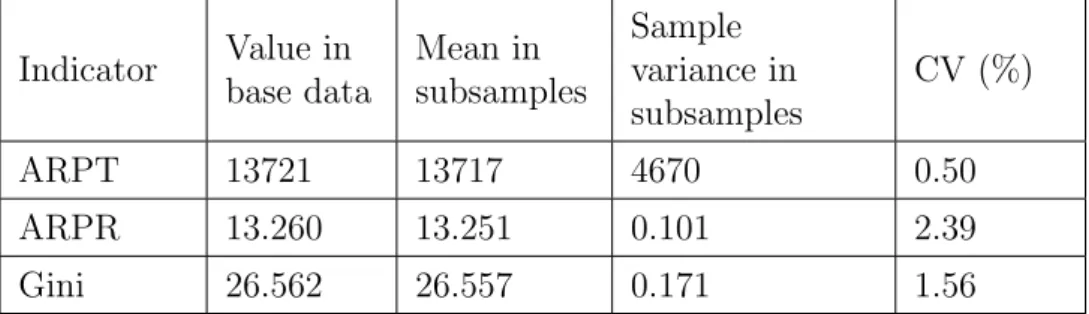
Table 1 contains statistics for the three poverty and inequality indicators as calculated from the 1,000 subsamples. We can see that the means of the values in the samples are very close to the real values calculated from the base data set, as is expected. The variances are relatively small with coefficients of variation being under 3% for all of the indicators.

Table 1: Sample statistics for the three indicators of interest

Indicator Value in base data Mean in subsamples Sample variance in subsamples CV (%) ARPT 13721 13717 4670 0.50 ARPR 13.260 13.251 0.101 2.39 Gini 26.562 26.557 0.171 1.56

Tables 2 and 3 contain statistics for the linearization and bootstrap variance estimates calculated from the 1,000 subsamples. From Table 2 it can be seen that on average the variance estimates obtained by both methods are about the same or slightly higher than the empirical variances shown in Table 1 for all of the three indicators. However, the medians for the variance estimates for the Gini coefficient differ noticeably from the means, being significantly lower than the empirical variance.

(40)

In the case of the Gini coefficient there is almost no difference between the two methods, but for the ARPT and the ARPR the estimates obtained by linearization have a markedly lower standard deviation than the bootstrap estimates. This difference is also apparent from Table 3 that shows that the linearization estimates have a lower relative root mean square error and coefficient of variation for the ARPT and the ARPR.

Table 2: Basic statistics for the variance estimators

Indicator Variance

estimator Mean Median

Standard deviation ARPT Linearization 5254 5248 234 Bootstrap 5273 5225 799 ARPR Linearization 0.100 0.100 0.003 Bootstrap 0.108 0.106 0.012 Gini Linearization 0.177 0.120 0.173 Bootstrap 0.179 0.124 0.174

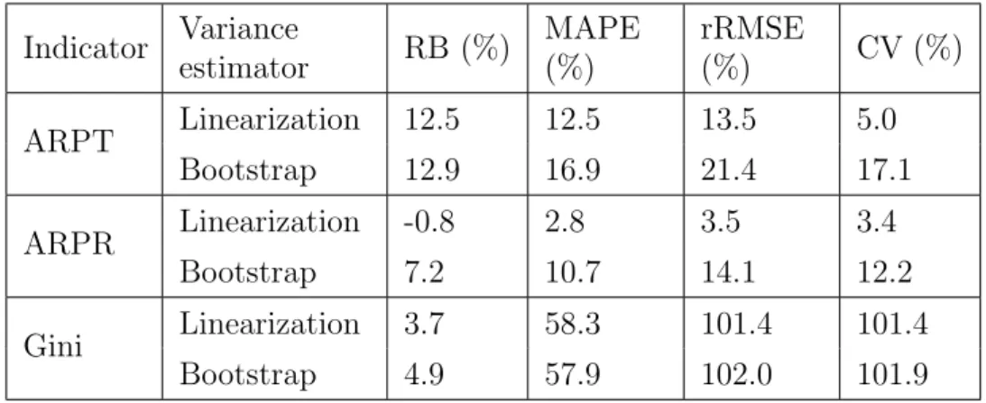
Table 3: Relative statistics for the variance estimators

Indicator Variance estimator RB (%) MAPE (%) rRMSE (%) CV (%) ARPT Linearization 12.5 12.5 13.5 5.0 Bootstrap 12.9 16.9 21.4 17.1 ARPR Linearization -0.8 2.8 3.5 3.4 Bootstrap 7.2 10.7 14.1 12.2 Gini Linearization 3.7 58.3 101.4 101.4 Bootstrap 4.9 57.9 102.0 101.9

(41)

Out of the three indicators of interest, the variance of the ARPR seems to be the easiest to estimate, with the linearization method in particular giving very accurate and precise estimates. The variance estimates for the Gini coefficient, on the other hand, have a very large variance in both cases with coefficients of variation of over 100%. The positive bias in estimating the variance of the ARPT is also relatively large with both methods.

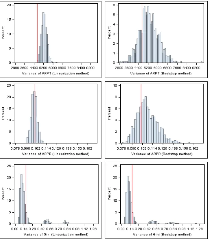
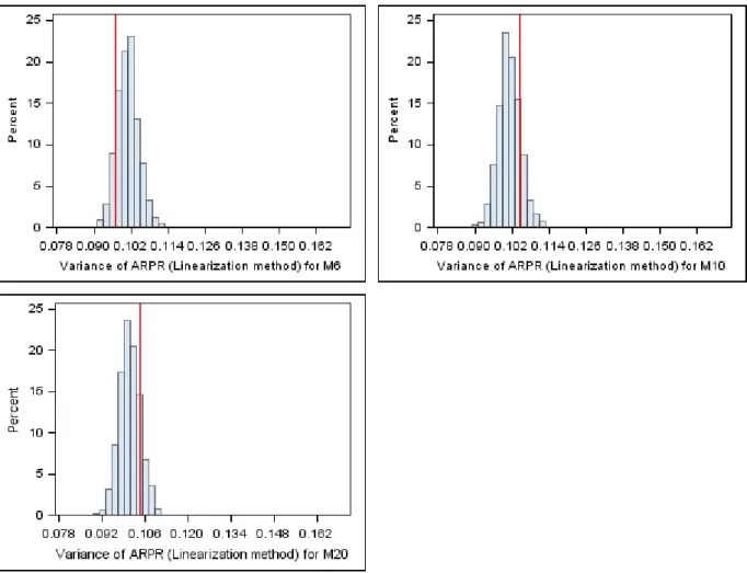
Histograms for the distributions of variance estimates are presented in Figure 3 and are reproduced in the Appendix in greater detail. The red lines are the empirical Monte Carlo variances for the corresponding indicators. For the ARPT and the ARPR it is clear that the bootstrap variance estimates are more widely distributed than the linearization variance estimates, meaning that the linearization approach gives better results. The positive bias in the variance estimates of the ARPT that was noted before is also apparent from the histograms.

The distribution of the estimates for the variance of the Gini coefficient is clearly asymmetrical for both approaches, with the bulk of the estimates falling short of the empirical Monte Carlo variance and with a few very high estimates.

(42)

Figure 3: The distribution of the linearization and bootstrap variance estimates for the three indicators. The red line is the empirical Monte Carlo variance.

(43)

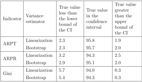
Table 4: Coverage of the 1000 confidence intervals constructed with estimated variances Indicator Variance estimator True value less than the lower bound of the CI True value in the confidence interval True value greater than the upper bound of the CI ARPT Linearization 2.3 95.8 1.9 Bootstrap 2.3 95.7 2.0 ARPR Linearization 3.2 94.3 2.5 Bootstrap 2.9 95.1 2.0 Gini Linearization 5.7 94.0 0.3 Bootstrap 5.4 94.3 0.3

Table 4 gives the coverage of the 95% confidence intervals constructed with the different estimated variances. In the ideal case we would like to see 95% of the confidence intervals contain the true parameter value, with 2.5% of them being too low and another 2.5% being too high. The confidence intervals for the ARPT and the ARPR perform quite well in this regard, but for the Gini coefficient it is much more likely than we would like that the lower bound of the confidence interval is higher than the true parameter value. However, the coverage of the confidence intervals is still about 95%.

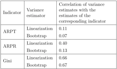
This anomaly in the confidence intervals is caused by the correlation between the estimate for the Gini coefficient and its variance estimate shown in Table 5. The high correlation means that in those subsamples where the Gini coefficient is estimated as being high, its variance estimate is also high and the resulting confidence interval is likely to cover the real value. Likewise, the subsamples that give low estimates for the Gini coefficient also give low variance estimates and the resulting confidence interval is less likely to cover the real value. The same phenomenon can also be seen to a lesser extent with the ARPT and the ARPR.

I assumed the notable outliers in Gini coefficient variance estimates were due to some high outlier incomes in the base data set that had a

Uncertainty in microsimulation : Assessing sampling variability in inequality and poverty indicators through variance estimation