Robust hedging in incomplete markets

(1)

Robust hedging in incomplete markets

Citation for published version (APA):

Shen, S., Pelsser, A., & Schotman, P. (2019). Robust hedging in incomplete markets. Journal of Pension

Economics & Finance, 18(3), 473-493. https://doi.org/10.1017/S1474747218000069

Document status and date: Published: 01/07/2019 DOI:

10.1017/S1474747218000069

Document Version:

Publisher's PDF, also known as Version of record Document license:

Taverne

Please check the document version of this publication:

• A submitted manuscript is the version of the article upon submission and before peer-review. There can be important differences between the submitted version and the official published version of record. People interested in the research are advised to contact the author for the final version of the publication, or visit the DOI to the publisher's website.

• The final author version and the galley proof are versions of the publication after peer review.

• The final published version features the final layout of the paper including the volume, issue and page numbers.

Link to publication

General rights

Copyright and moral rights for the publications made accessible in the public portal are retained by the authors and/or other copyright owners and it is a condition of accessing publications that users recognise and abide by the legal requirements associated with these rights.

• Users may download and print one copy of any publication from the public portal for the purpose of private study or research. • You may not further distribute the material or use it for any profit-making activity or commercial gain

• You may freely distribute the URL identifying the publication in the public portal.

If the publication is distributed under the terms of Article 25fa of the Dutch Copyright Act, indicated by the “Taverne” license above, please follow below link for the End User Agreement:

www.umlib.nl/taverne-license Take down policy

If you believe that this document breaches copyright please contact us at:

repository@maastrichtuniversity.nl

providing details and we will investigate your claim.

(2)

Robust hedging in incomplete markets

SALLY SHEN

Global Risk Institute, 55 University Avenue, Toronto, ON M5J 2H7, Canada and Network for Studies on Pensions, Aging and Retirement

(e-mail:sshen@globalriskinstitute.org) ANTOON PELSSERANDPETER SCHOTMAN

Network for Studies on Pensions, Aging and Retirement and Department of Finance, Maastricht University, PO BOX 616, 6200 MD Maastricht, The Netherlands

Abstract

We considered a pension fund that needs to hedge uncertain long-term liabilities. We modeled the pension fund as a robust investor facing an incomplete market and fearing model uncertainty for the evolution of its liabilities. The robust agent is assumed to minimize the shortfall between the assets and liabilities under an endogenous worst-case scenario by means of solving a min–max robust optimization problem. When the funding ratio is low, robustness reduces the demand for risky assets. However, cherishing the hope of covering the liabilities, a substantial risk exposure is still optimal. A longer investment horizon or a higher funding ratio weakens the investor’s fear of model misspeciﬁcation. If the expected equity return is overestimated, the initial capital requirement for hedging can be decreased by following the robust strategy.

JEL CODES:G11, G13

Keywords: Model uncertainty, robust optimization, incomplete market, dynamic hedging, expected shortfall.

1 Introduction

After the 2008 global financial crisis, the performance of US pension funds has remained depressed. The poor solvency situation has been driven by a declining discount rate and also a fall in equity prices. Since 2012, funding ratios (asset values divided by projected benefit obligations) of the top 100 largest US corporate defi ned-benefit pension plans have not rebounded. More importantly, projected future funding ratios show a wide range of uncertainty for the next 2 years.1_{This raises the question of} how to price and hedge downside risks when confronted with fragile beliefs about the likelihood of different funding ratio scenarios.

1 _{Based on the data obtained from Milliman Pension Fund Index http://us.milliman.com/p}_ﬁ_{/us.milliman.} com for the Milliman 100 funding index ratio from the beginning of 2012 to July 2017 and projections from August 2017 to 2018.

doi:10.1017/S1474747218000069 First published online 16 March 2018

https://www.cambridge.org/core

. Universiteit Maastricht

, on

21 Oct 2020 at 10:46:54

, subject to the Cambridge Core terms of use, available at

https://www.cambridge.org/core/terms

(3)

Pricing and hedging pension or insurance liabilities faces two problems. First, the market is incomplete. Liability risks are typically not–or not actively – traded in thefinancial market. According to EIOPA (2011)2_{, the two largest components of} liability risks are market risk and life risk, which account for 67.4% and 23.7% of the diversified Basic Solvency Capital Requirement (SCR), respectively. However, these risks are not fully traded. Interest rate risk, one of the dominant market risks, is only partially traded in thefinancial market. Pension funds and insurance compan-ies are often confronted with ultra-long-term commitments with maturitcompan-ies of more than 50 years. However, the longest dated government bonds even in developed mar-kets such as the US, UK, and Canada are up to 30 years. In developing marmar-kets (such as Asia, Eastern Europe, and South America), long-term government bonds with maturities more than 10 years barely exist.

Life risk faces more serious market incompleteness problem, because mortality-linked securities in general have very low liquidity. For instance, longevity risk, the risk that insurers might live longer than anticipated, is the most important component of life risk. Turner (2006) shows that, in 2005, 2460 billion liabilities are associated with longevity risk in the UK. However, longevity risk had never been securitized until early 2000s. In the past decade, a limited number of mortality-linked products such as the longevity bond (see Blake and Burrows (2001)) have been proposed, while only a very small amount (<1%3_{) of longevity risk can be hedged.}

The second problem concerns model parameter uncertainty in hedging liability risks. On the liability side of the balance sheet, longevity has been improving unpre-cedentedly in the past few decades in an unpredictable way (see, e.g. Benjamin and Soliman, 1993; McDonald et al., 2006). An inaccurate mortality estimation makes pricing and hedging liability risks much more difﬁcult and less reliable. Early work by Lee and Carter (1992) has been considered as the nucleus of modeling the dynam-ics of the mortality rate. Several plausible extensions of the Lee–Carter model, such as an incorporation of heterogeneous cell level (Liet al., 2009), age-dependent factors (Cairns et al., 2006), and structural changes (Coelho and Nunes, 2011; Van Berkum et al., 2016), introduce substantial uncertainty on the trend in longevity and hence in the growth in liabilities.

On the other side of the balance sheet, the expected asset return is notoriously difﬁ -cult to estimate from historical data. Merton (1980) argues that it is difﬁcult to esti-mate expected returns from time series of realized stock return data. The standard deviation of the historical average return isσ/√T whereσis the standard deviation of annual returns and T is the number of years. For example, if T= 100 and

σ=16%, then the standard error of the equity premium is 1.6%, which leads to an approximate 95% conﬁdence interval span of 6.3%(+1.96×1.6%). Although the interval shrinks with the square root of the sample size for estimation, it is difﬁcult to maintain the same data generating process throughout the entire period. The investor is therefore exposed to estimation error in the expected asset returns.

2

EIOPA (2011) is short for European Insurance and Occupational Pension Authority (2011). See https:// eiopa.europa.eu/Publications/Reports/QIS5_Report_Final.pdfReport on the ﬁfth quantitative impact study (QIS5) for Solvency II.

3 _{See Blake and Burrows (}₂₀₀₁_).

, on

21 Oct 2020 at 10:46:54

(4)

Doubts about the accuracy of the model makes an agent treat it as an approxima-tion of an unknown true model. She wants her decision rules to work well over a set of models in the neighborhood of the approximating model. Our aim is to develop a hedging strategy for an agent who faces uncertainty about the expected return on the assets as well as uncertainty about the expected growth in liabilities. We adopted the robust control theory to deal with the fear of model uncertainty. The agent who worries about model misspeciﬁcation looks for a prudent policy that is resilient to fra-gile beliefs about the likelihood of the state variables. Such decision rules are called robust policies. We introduced a robust hedging strategy along the lines of Hansen and Sargent (2007) to hedge undiversiﬁable downside risks.

The robust optimal hedging strategy that we propose takes both downside risks as well as market incompleteness into account for an agent who fears parameter uncer-tainty. The robust agent is assumed to minimize the shortfall between assets and liabilities under a statistically plausible worst-case scenario by means of solving a min–max robust optimization problem. The robust model includes three crucial ele-ments. The first is downside risk, which we define as expected shortfall. In a static model, the expected shortfall between the assets and the liabilities can be valued as the payoff of an exchange option, which swaps the optimal value of the asset for the price of the liabilities. The second element is incomplete markets. We introduced two uncorrelated risk drivers in our model, one hedgeable and the other not hedge-able. The unhedgeable risk captures the incompleteness of the market. The asset mar-ket is exposed to hedgeable risk only, but the liability side is exposed to both types of risk. The third element is parameter misspecification. Following Anderson et al.

(2003) and Maenhout (2004), we introduced drift distortions on the Brownian motions to represent parameter misspeciﬁcation. These drift distortions perturb the true data generation process of approximate models. Economically, an additional drift on the Brownian motion can be understood as the unobservable market price of risk, which relates to Cochrane and Saa-Requejo (2000)’s concept of Good Deal Bounds (GDB). Technically, drift distortions measure the discrepancies between alter-native probability distributions. A closely related idea appears in Cvitanić and Karatzas (1999), but in their model, liabilities only depend on the value of market instruments.

We solved the robust hedging problem in both a static and a dynamic environment. In both cases, the robust policy is more conservative than the naive policy. This result is in line with Brennan (1998). When the funding ratio is low, agents will increase the risk exposure to the stock market so as to gamble their way out of trouble (see also Ang et al., 2013). The more the investor invests in the risky asset, the more she becomes exposed to estimation uncertainty. The robust agent is particularly afraid of a downside shock with the risky assets and hence she will put less wealth in the stock market compared with the agent who disregards the estimation uncertainty. We also found that for both the robust as well as the non-robust policy, the risky por-tion of the portfolio decreases with the hedging horizon when the funding ratio is low, andvice versawhen the funding ratio is high. The impact of the preference for robust-ness depends on the hedging horizon as well as the funding ratio.

, on

21 Oct 2020 at 10:46:54

(5)

More importantly, we evaluated the robust policy by means of comparing its expected loss with the non-robust policy. The loss function is deﬁned as the difference between the cost of hedging conditional on the estimated expected return and the true minimum cost. The beneﬁts of a robust policy are twofold. First, the robust policy is less sensitive to the estimated parameters. Second, the robust policy has a lower hedg-ing cost than a naive policy, under a range of alternative parameter values.

One strong assumption in this paper is that the investors only fear a subclass of model misspeciﬁcation, namely the drift parameters of the state variables instead of the general model uncertainty problem. Similar to Maenhout (2004), we reduced the general model uncertainty problem to a ﬁrst-moment parameter uncertainty problem.

Another strong assumption in our work is that the investors do not engage in any learning. Brennan (1998) incorporates learning with parameter uncertainty and ﬁnds that after learning, high-risk-averse investors are more conservative with their invest-ment, but low-risk-averse investors allocate more wealth on risky assets. Wang (2009) incorporates income growth rate uncertainty with Bayesian learning for a consumption-saving and optimal portfolio choice problem and ﬁnds that learning induces additional precautionary saving.

Numerous studies deal with asset allocation problem for pension plans. Seminal work by Sharpe and Tint (1990) develops a surplus management approach in which funds care about assets minus liabilities. Detemple and Rindisbacher (2008) extend this framework to a dynamic setting. Anget al.(2013) add an additional pen-alty function at the mean-variance framework of Sharpe and Tint (1990). The penalty function, which is the shortfall between the asset and liabilities, is the same as our objective function, to which we add model uncertainty.

A related study on model uncertainty by Garlappiet al.(2006) considers a mean-variance portfolio choice of a robust investor who has imperfect information on the expected return. They use multi-prior approach advocated by Gilboa and Schmeidler (1989), and they alsoﬁnd that allowing for parameter uncertainty reduces the portfolio weights on risky assets over time. Luo (2016) considers both model uncertainty and state uncertainty under decision-making. State uncertainty refers to incomplete information about the true value of the state due to sluggishness of the market. In this paper, we do not deal with state uncertainty, but the likelihood over the state variables.

2 Model

We considered a continuous-time incomplete market with a finite trading horizon [0,T]. The risk is modeled by a filtered probability space (Ω,F,P), on which are defined two uncorrelated risk factors, a hedgeable risk W1t and an unhedgeable

riskW2t. BothW1tandW2tare univariate standard Brownian motions and we

con-sidered{Ft:t[[0,T]}as the completion of theﬁltration generated byW1tandW2t.

A hedgeable risk means we can replicate the payoff of this kind of risk perfectly. The payoff for an unhedgeable risk is not replicable because it is not traded.

, on

21 Oct 2020 at 10:46:54

(6)

2.1 Asset and liability model

On the asset side, we have a risk-free money-market accountBt, which earns a

deter-ministic risk-free rate of interestr, sodBt=rBtdt. We also have a stock market. The

stock price follows a geometric Brownian motion process dSt=μStdt+σStdW1t. The agent can only invest in the money-market account and the stock market. Denote the value of the assets at timetbyAt. The investor puts an amountwtAtin

the stock market at time t. The remaining part of the assets (1−wt)At is put into

the money-market account. The asset diffusion process follows as

dAt = (r+wt(μ−r))Atdt+wtσAtdW1t, (1) wherewtis the possibly time-varying hedging strategy. We do not set a constraint on

wt, therefore short positions are allowed.

The liability is exposed to both hedgeable riskW1tand unhedgeable riskW2t. We

assumed that the diffusion process of the liability Lt follows an exogenously given

geometric Brownian motion with constant drift term and constant volatility,

dLt=a Ltdt+b Lt ρdW1t+ 1−ρ2 dW2t , (2)

whereais the drift of the liability andbis its volatility. The non-traded risk driver,

dW2t, represents the incomplete part of the market. We introduced a correlation

par-ameterρ∈[−1, 1] between asset risk and liability risk. It controls the risk exposure to

W2tof the liability. Ifρ= ±1, then the non-traded riskW2tdisappears from the

liabil-ity side. The liabilliabil-ity in this case can be perfectly hedged by a replicating portfolio. We are interested in the case whenρis strictly between−1 and 1.

2.2 Robust asset and liability model

We used the Hansen and Sargent’s (2007) framework to integrate the preference for robustness to the asset-liability models (1) and (2). With a preference for robustness, the agent treats (1) and (2) as an approximate model for the unknown true state evo-lution ofAtandLt. We limited the parameter uncertainty to the drift termsμanda

only, and assumed that the volatilitiesσ and bare known. The approximate model only provides an estimated value of the drift terms, but the growth rate of liabilities and the expected return are imprecisely estimated and subject to estimation error. However, the constant volatility parameterσcan potentially be estimated using high-frequency observations, and is therefore not subject to parameter estimation error.

In the Hansen and Sargent’s framework, the robust model contains an unknown drift term on the Brownian motion. In our case, the Brownian motions dW1tand

dW2t in (1) and (2) are replaced by dW1t+λ1tdt and dW2t+λ2tdt. The two drift

terms λ1tandλ2tare deﬁned as two perturbation time-series processes that quantify

the misspeciﬁcation of the underlying model. The values of λ1t and λ2t shift the

mean distribution of the asset and the liability diffusion process by a unit of wtσλ1t

andbρλ1t+b

1−ρ2

λ2t, respectively. Hence, they specify a set of alternative measures referring to different speciﬁcations of the stochastic process known as a Girsanov ker-nel. The misspeciﬁed expected return also generates an error in the market price of

, on

21 Oct 2020 at 10:46:54

(7)

risk. The perturbed evolution of the state variables is given by: dAt= (r+wt(μ−r))Atdt+wtσAt(dW1t+λ1tdt), (3a) dLt=a Ltdt+b Lt ρ(dW1t+λ1tdt) + 1−ρ2 dW2t+λ2tdt ( ) . (3b) The perturbation of the model is bounded by an uncertainty set S. The larger the uncertainty setS, the more pessimistic the agent is about the accuracy of the under-lying model. To describe the uncertainty set, we introduced some additional notation. Letδbe the vector of the estimated drift terms,

δ= μ_a

and letδ0be the true drift. Thenδ−δ0is the estimation error,

δ−δ0= σ 0 bρ b1−ρ2 λ1t λ2t =Γλt.

The estimation errorδ−δ0is asymptotically normal with mean zero and covariance matrix (Σ/N), whereNis the length of a (hypothetical) sample used for estimation and

Σ=ΓΓ′₌ σ2 bρσ bρσ b2

.

We obtained the uncertainty set based on the property that (δ−δ0)′(Σ/N)−1(δ−δ0) is aχ2distribution with two degrees of freedom,χ2(2). Denoting the critical value atα signiﬁcance level as CV_α, we then have a probability of 1−αthat

δ−δ0

( )′_Σ−1 _δ₋_δ 0

( ) ≤κ2_, ₍₄₎

whereκ2= (CV_α/N). Equation (4) provides a natural boundary of the perturbation parameters. Simplifying (4) further, we get

Γλt

( )′_ΓΓ′ −1 Γλt

( ) =λ′

tλt≤κ2. Hence our uncertainty set is as follows,

S= λ1t,λ2t|λ21t+λ22t≤κ2

. (5)

Our uncertainty set has a circular shape inλtspace centered by zero. Given the

esti-matesδa credibility region for the true value,δ0can be constructed as

δ0[{δ+Γλt|S}. (6)

The true drift termδ0is constrained by an ellipsoid uncertainty set centered byδand it can be at any point within this set. The size of the uncertainty set depends on the sign-iﬁcance levelαand the hypothetical sample sizeN. If the agent has inﬁnite observa-tions, then the uncertainty set shrinks to the point estimateδ.

Our stylized uncertainty set is related to the GDB proposed by Cochrane and Saa-Requejo (2000). Equation (4) can be understood as the GDB constraint in which we put a limit on the unobservable part of the market price of risks,λ1tand λ2t. The uncertainty set we proposed differs from the GDB in the way in which our

uncertainty set is derived from the econometric estimation error. The uncertainty

, on

21 Oct 2020 at 10:46:54

(8)

set parameter κ depends only on the statistical quantities, α and N. However, the GDB method is inspired by an economic belief that the total market price of risk in an incomplete market has to have limits.

2.3 Robust optimization problem

Utility is deﬁned as a function of the terminal value forATandLTat the terminal date

T. The optimal hedging strategy maximizes the utility functionE[U(AT,LT)|Ft]. As a benchmark, we deﬁned the naive policywnaas the hedging strategy that does not

con-sider model misspeciﬁcation.

The uncertainty averse agent looks for a robust hedging policy that works well over a set of models. The robust hedging policy is deﬁned as

max wt _λ1tmin,λ2t[S

E[U A( T,LT)|Ft]. (7)

The max–min optimization problem is a two-player zero-sum game, see Anderson

et al.(2003). This is a sequential game between the decision-maker and a malevolent nature. Player 1, the robust agent moves ﬁrst by choosing investment decisions to maximize the utility function at time t, and then player 2 (the imaginary nature) picks the worst state of nature for player 1 by making an instantaneous choice of

λ1t and λ2t, given player 1’s choice. In other words, the agent is maximizing while

nature is minimizing.

3 Static robust optimization

In the following two sections, we will show how to solve the robust optimization prob-lem and how the robust solution differs from the naive one, and also how we can beneﬁt from the robust decision. We started with the relatively simple static case, where both agent and nature only make decisions now att= 0 without rebalancing until the terminal dateT. The static case is technically easy to solve, but still provides us with some intuition about the robust policy. However, the static solution may not be optimal. With a dynamic solution bothwtandλ1t,λ2tare time-series processes.

Given the information at timeT, our hedging strategy is deﬁned over the hedging error LT−AT at a predetermined timeT. Our utility function takes the form of the

shortfall risk U A( T,LT) = −[LT−AT]+, which speciﬁes the downside risk on the liability shortfall. The lower the shortfall risk, the higher the agent’s utility will be. The naive optimization problem is given by

min

wt E[(LT−AT)

+_] ₍₈₎

and the robust optimization is min

wt _λ1maxt,λ2t[S

E[(LT−AT)+]. (9)

In the static case, the order of the two players is interchangeable. According to the saddle-point existence Theorem mentioned in Delbaen (2002) and Rockafellar (1976), the optimal solution of (9) is a saddle point, since both control variables

, on

21 Oct 2020 at 10:46:54

(9)

are constrained by a convex set and the value function is bilinear. Hence (9) and its dual problem max

λ1t,λ2t min

wt E[(LT −AT)

+_]_{have the same optimal solution.}

3.1 Static solution

To facilitate calculation, let

μS =μ+σλ1, (10a) μA=r+w(μS−r), (10b) μL=a+bρλ1+b 1−ρ2 λ2, (10c)

represent the drift terms of the stock market, the asset and the liability, respectively. Note thatμSdepends onλ1;μAdepends on bothwandλ1; andμLdepends onλ1andλ2. In the static case, our criterion functionE[(LT−AT)+] is very similar to the value of

an‘exchange option’, which exchanges one asset for another at timeT. This type of option has been valued in Margrabe (1978). The problem in our case is more compli-cated, because we are in an incomplete market, which means the equivalent martin-gale is not unique, or in other words, the so-called risk-neutral ℚ measure is not unique, but depending onλ1andλ2.

There are many ways to solve this static criterion function. We used the change of probability measure technique. The analytical solution of our objective function under the static case is given by

E (LT−AT)+ =LΦ(−d2) −AΦ(−d1) =L Φ(−d2) −CΦ(−d1) , (11) where L=L0exp μLT , A=A0exp(μAT), C=C0exp μA−μL T , and d1= lnC+σ 2 C 2 T σC T √ , d2=d1−σC T √ ,

whereC0= (A0/L0) is the current funding ratio. The functionΦis the standard normal distribution function. If the funding ratio is less than one, the fund is facing a solvency risk. For givenλ1andλ2, the optional hedge disregarding the preference for robustness is the solution of theﬁrst-order condition for maximizingEL[(1−CT)+] with respect

tow, ∂ Φ(−d2) −CΦ(−d1) ∂w = −Φ(−d1)C μ−r T+Cϕ( )d1 T √ wσ2−bρσ σC = 0, (12) where functionϕdenotes the standard normal density function. Note that−Φ(−d1) is the δ of the Black–Scholes (BS) put-option that is always less than zero, and

, on

21 Oct 2020 at 10:46:54

(10)

Cϕ( )d1

T √

denotes theνof the BS option that is always positive. Therefore, we see from (12) that the optimal w strikes a balance between the ‘δ effect’ that reduces the value of the option and the ‘ν effect’ that increases the value of the option. There is a special case when μ=rwhere the ‘δeffect’disappears and the optimalw

is then given by the minimum variance solutionw= (bρ/σ).

3.2 Static robust portfolio choice

Based on the analytical solution (11), we solved the static robust optimization prob-lem numerically. As a benchmark scenario, we assumedμ= 0.04,σ= 0.16,r= 0,a= 0,

b= 0.1,ρ= 0.5. We assumed that the stock returnμis higher than the liability return

a. As we discussed in Section 2.2, the uncertainty set parameterκdepends on the sign-ificance levelαand the sample sizeN. Hence, it isfixed and state variable independ-ent. For a significance level α= 0.05, the correspondingχ2 value with 2 degrees of freedom is 5.99. The choice of κ is also based on an implicit assumption that the risk premium (μS−r/σ) is always positive, which means (μ−r/σ) +λ1> 0. Given the uncertainty set S, the absolute value of λ1is bounded with |λ1|∈[−κ, κ], hence κ has to satisfy the condition thatκ≤((μ−r)/σ) = 0.25 in order to guarantee a positive risk premium. Therefore, we set κ= 0.25 for the benchmark scenario. Alternatively, using the significance level, the sample size Nhas to be larger than 96 years so as to satisfy this implicit assumption.

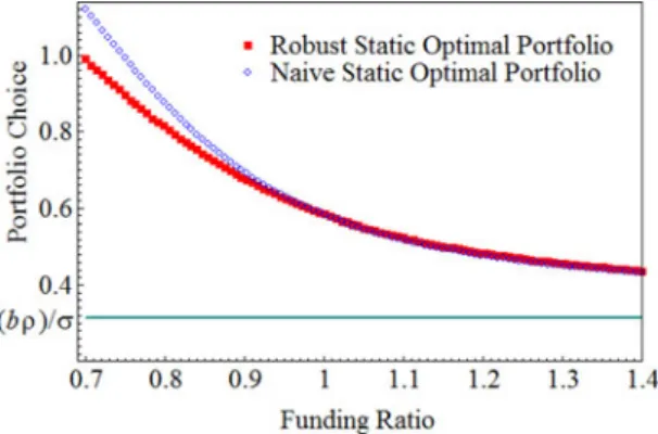
InFigure 1, we show the static optimal portfolio choice at timet= 0 as the function of the current funding ratio, C0. When there is underfunding, the robust and naive policies differ. Both take substantial risk betting on the chance to meet the liability, but the robust portfolio is more conservative than the naive one. For example, if the current funding ratio equals 80%, then the robust policy will reduce the risky asset exposure by approximately 6% relative to the naive policy. The robustness effect diminishes ifC0goes up. The two curves converge to the minimum-variance hedging ratio ((bρ)/σ) = 0.3125 ifC0is sufficiently large. The resulting volatility becomesb(1−ρ2), which is the unhedgeable part of the liability risk. Also, this position neutralizes theλ1 effect such that the misspecification of asset return does not influence the performance of hedges. Therefore, the robust hedges are not always more conservative than naive hedges. If the fund is already balanced – or even overfunded with C0≥1 – the two policies are almost identical.

The decision of nature is displayed inFigure 2. We showedλ1andλ2as a function of the present funding ratioC0. To facilitate the comparison, we put the two pertur-bations in one graph. We found that λ1is negative at any funding ratio level but is close to zero when C0 is high; λ2 is always positive and converges to κ. We also found that the optimal choice of λ1 and λ2 is always on the circle λ12+λ22=κ2,

which means the worst-case scenario is always at the boundary of the uncertainty set.

Figure 2shows that a negativeλ1and a positiveλ2lead to the worst-case scenario. This is because the agent is afraid that the true expected asset return is lower than the estimated value, and the true liability return is higher than the estimated result. The resulting negativeλ1represents the fear of an overestimated asset return. Hence, the absolute value of λ1is increasing with the exposure to the stock market, w. We

, on

21 Oct 2020 at 10:46:54

(11)

know fromFigure 1that risk exposure and the funding ratio are negatively related. The lower the funding ratio, the higher the risk exposure will be and therefore the more negative the value ofλ1will be. In contrast, if the funding ratio is sufﬁciently high, both the λ1 penalty as well as the weight in the risky asset are smaller. The penalty term λ1 also plays a role in the liability return. A negative λ1 can beneﬁt the agent by reducing the expected liability return. To capitalize on the fear of an increase in the liability return, nature chooses a positiveλ2 so as to compensate for the negative effect fromλ1and to increase the liability growth, making the liabil-ity more costly.

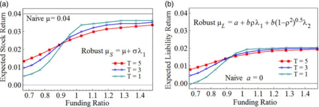
We further examined how the perturbation terms impact the expected returns.

Figure 3displays both the naive and robust mean rates of the stock return and the liability return as functions ofC0. Without the preference for robustness, both drift terms are constant. However, if the investor is aware of the model misspeciﬁcation, the perturbed expected stock return is dragged down by |σλ1| due to the negative impact of λ1. Despite the mixed sign of λ1 and λ2, the worst-case liability drift is pushed up by|bρλ1+b

1−ρ2

λ2|since the positive effect of λ2dominates the drift distortion. In general, the robust policy differs from the naive one in the sense that the robust agent requires an additional guarantee on top of the naive contract in order to neutralize the estimation error. In other words, the robust policy needs more capital to hedge downside risks.

Figure 1. Static optimal portfolio choice. Thisﬁgure compares the robust and naive static optimal hedging policies. The investor makes an investment decision at time t= 0 with given current funding ratioC0 so as to minimize the expected shortfall at

time periodT. The naive policy relies completely on the estimation parameters. The robust policy takes the parameter uncertainty into consideration and insures against the worst-case scenario. The horizontal axis depicts the present funding ratio. The results are based on the benchmark estimation parameters μ= 0.04, σ= 0.16, r= 0, a= 0, b= 0.1, ρ= 0.5, κ= 0.25, andT= 5. https://www.cambridge.org/core . Universiteit Maastricht , on 21 Oct 2020 at 10:46:54

(12)

3.3 Policy evaluation

The robust policy is less sensitive to the parameter misspecification. In this section, we will show how and when the agent can benefit from the robust policy. LetQ(w,δ) be the cost of hedging following a particular policyw, whereδis the assumed value of the drift parameters. In our case, the cost of hedging is defined by

Q w( ,δ) =E (LT−AT)+|w,δ

. (13)

The optimal hedging policy has a costq(δ) =min

w Q w( ,δ)for given δ. Letδ0be the true value of δ, and denote q(δ0) as the minimum hedging cost when the investor implements the associated optimal hedging policy w0 under the true value δ0. Any other alternative hedging policies wa(wa=w0)have higher expected shortfall.

Deﬁne the loss function K(wa|δ0) as the difference between the cost of hedging

fol-lowing a suboptimal policywaand the true minimum cost. The‘cost of hedging’here

is deﬁned as the initial wealth required to obtain a particular level of expected short-fall, denotedQ(wa,δ0), which gives the loss function

K w( a|δ0) =Q w( a,δ0) −q(δ0). (14)

If δ≠δ0, the agent is facing estimation error, thereforewa≠w0andK(wa|δ0) > 0. The agent does not know the true value of the drift termsδ0. Given the estimated drift termsδ, she can choose between two alternative hedging policies, a robust policy

wroband a naive policywna. At the benchmark scenario when the present funding ratio

C0=80%, the solutions arewrob= 0.81 andwna= 0.87. When C0=90%, we found

that wrob= 0.67 and wna= 0.69. The robust policy will perform better than the

Figure 2. Static optimal perturbations λ1 and λ2. This ﬁgure depicts the optimal λ1 and λ2 as functions of the

present funding ratio C0 under the benchmark scenario

with μ= 0.04, σ= 0.16, r= 0, a= 0, b= 0.1, ρ= 0.5, κ= 0.25, and T= 5. Nature makes decisions of λ1 and λ2 at

time 0 under the constraint λ2₁+λ2₂≤κ2_{so as to maximize}

the expected shortfall at periodT.

, on

21 Oct 2020 at 10:46:54

(13)

naive policy, if

K w( rob|δ0),K w( na|δ0). (15)

We displayed the loss indifference curves inFigure 4when the present funding ratio is 80% and 90%. Thex-axis andy-axis represent the true value of liability returna0 and asset returnμ0, respectively. The point [a= 0,μ= 0.04] represents the estimated expected return δ. We also displayed the ellipsoid uncertainty set of the true drift termδ0in theﬁgure.

WhenK(wrob|δ0) =K(wna|δ0), the two policies require the same amount of wealth to

hedge. In the region below the curve for both scenarios (whenC0=80%and 90%), the

robust policy requires less initial wealth than the naive policy to hedge a certain amount of expected shortfall. We call this area the robust policy’s‘beneﬁcial region’. Hence, we can conclude that when the true drift termδ0is overestimated, the robust policy performs better.

This beneficial region is positively related to the present funding ratioC0. Since the additional cost of hedging by following a robust policy increases asC0decreases, a lowerC0leads to a smaller beneficial region. When liabilities are covered, the differ-ence between a robust and a naive policy is subtle and the robust investor’s beneficial region should also be larger.

3.4 Sensitivity analysis

The correlation parameterρ, representing the completeness of the market, plays an important role in the model. Ifρ= ±1, andλ1=λ2= 0, then the market becomes com-plete and the unhedgeable risk driver W2 does not play a role. In this section, we investigated how sensitive the optimal hedges are with respect to a change ofρ.

InFigure 5, we show an extreme case whenρ= 1. The non-traded risk driverW2 disappears from the liability diffusion process, and the perturbation parameter λ2 does not play a role either. Nature can only control λ1 to maximize the expected

Figure 3. Mean rate of stock and liability return with and without the preference for robustness. This ﬁgure displays the expected stock and liability returns before and after considering parameter uncertainty as functions of the present funding ratio. Panel 3a comparing the robust stock drift μS=μ+σλ1 with the naive drift term μS=μ. Panel 3b

comparing the robust liability drift term μL=a+bρλ1+b

1−ρ2

λ2 with the naive one

μL=aunder the benchmark scenario.

, on

21 Oct 2020 at 10:46:54

(14)

shortfall at periodT. The naive agent considers this as a complete market. However, the robust agent still faces another source of incompleteness, caused by model misspeciﬁcation.

With a low funding ratio, the robust policy deviates from the naive one much more severely compared with the benchmark case. When the asset risk and the liability risk are perfectly correlated, nature will choose a more negativeλ1so as to maximize the expected shortfall. Although a negativeλ1reduces the expected liability return as well, the liability drift term is less sensitive to the change of λ1 than the expected asset return, since σ>b. As a result, the robust investor’s fear of an overestimated asset return is stronger than the benchmark level.

In the case of overfunding, the two policies are identical. The hedging error vola-tility becomesσ2

C= wσ−bρ

2

. The investor can fully replicate the liability by follow-ing a δ-neutral strategy w= ((bρ)/σ) =62% if she has sufﬁcient assets. In that case, robustness does not play a role because theδhedge neutralizes theλ1effect.

InFigure 6, we show the two hedging policies as a function of correlation param-eter ρ. We displayed two scenarios, one when C0=80% and the other when C0=90%. The relation between the optimal portfolios and ρ is not monotone but

is hump shaped. This is because the volatility of the value functionσCis a quadratic

function ofρ.

The optimal portfolio initially increases withρfor both policies because the liability is more exposed to the tradable risk driverW1. Therefore, the risky portfolio has to increase as well, in order to hedge the traded liability risk. The optimal portfolio reaches the peak whereρmaximizes the total volatilityσC. After the peak, the risky

Figure 4. Loss function equivalent curves. The ﬁgure plots the indifference curve of the loss whenK(wrob|δ0) =K(wna|δ0).

y-axis is the true value of the expected stock returnμ0and

x-axis is the true value of the liability drifta0. The estimated

value isμ= 0.04 and a= 0. The solid-dot indifference curve represents the case when C0=80% and the open-dot curve

is the when C0=90%. In the region below the curve, the

robust policy outperforms the naive policy, and in the region above, it is the other way around.

, on

21 Oct 2020 at 10:46:54

(15)

portfolio goes down withρ, because after the peak, any higher level of correlation will reduceσC. FromFigure 6, we can also see that the difference between the two policies

under the lower funding ratio is wider than under the higherC0.

4 Dynamic robust optimization

In this section, we will extend the problem to a dynamic strategy. The robust investor still aims to minimize the ﬁnal-period expected shortfall under the worst-case scen-ario, but instead of making a static portfolio choice, she is now considering a dynamic optimal portfolio. Nature also can rebalance her choice of (λ1t, λ2t) instantaneously

given the intertemporal decision of wt. We employed dynamic programming to

solve this robust optimization problem.

4.1 Dynamic programming

Deﬁne the indirect utility function V(At, Lt), which follows the min–max expected

utility given by (9). Both the investor and nature have a planing horizon of T. We omited the time subscripttfor notation convenience. Using Feynman–Kaç, we can derive the Hamilton–Jacobi–Bellman equation (henceforth HJB) or partial differen-tial equation (pde) for the investor’s min–max problem:

0=min w max_λ1,λ2 Vt+VAA r+w(μ−r) +wσλ1 +VLL a+bρλ1+b 1−ρ2 λ2 +1 2VAAw 2_σ2_A2₊1 2VLLb 2_L2₊_V ALbρwσAL− 1 2ν λ 2 1+λ22−κ2 , ( 16)

Figure 5. Sensitivity analysis withρ= 1. Theﬁgure depicts the optimal portfolio choice when ρ= 1. The remaining parameters stay at the benchmark level. The solid-dot line represents the robust policy and the empty-dotted curve is the naive policy. The naive agent considers such an economy a complete market, since the non-tradable risk driverW2is gone. However, the robust agent still stays in

the incomplete market, because the model misspeciﬁcation (λ1=0λ2=0) is also considered as another source of

market incompleteness.

, on

21 Oct 2020 at 10:46:54

(16)

where the partial derivative with respect to x is denoted as Vx. We formed a

Lagrangian function with multiplierνover the boundary condition:λ2₁+λ2₂≤κ2.4 By solving a linear system of equations based on the ﬁrst-order condition of (16) with respect to the strategy variables w, λ1, andλ2, we have

w∗ = − μ−r VAAν σ2 _V AAA2ν+VA2A2 −VALALbρσν+VLVAALbρσ σ2 _V AAA2ν+UA2A2 , (17a) λ∗1= − μ−r V2 AA2σ σ2 _V AAA2ν+V_A2A2 −bρ VALALVAA−VLLVAAA2 VAAA2ν+V_A2A2 , (17b) λ∗2= VLLb 1−ρ2 ν . (17c)

This is a partial solution. The Lagrange multiplierν, as well asVA,VAA, still need to

be solved numerically.

The sign of the optimalλ2must be positive since it increases the expected liability return but does not inﬂuence the pension asset. The sign ofλ1is ambiguous. A positive

λ1not only increases the liability but also the asset, but the net effect depends on the value of other input variables.

Figure 6. Sensitivity analysis with respect to ρ. The ﬁgure plots the optimal naive and robust hedging policies as a function of correlation parameterρ. We show two pairs of comparison: one with the present funding ratioC0of 80%,

and the other with C0=90%. The solid-dot curves

represent the robust policy and the empty-dot curves are the naive policy.

4

The Lagrangian multiplierνrelates to the time-consistent per-period constraint (6), which is different from the setup of Andersonet al. (2003). In Andersonet al. (2003), the last term of the HJB equation is replaced by a relative entropy function, 1/2θ λ2₁+λ2₂ which penalizes drift distortions. Although the two HJB equations look similar,θimplicitly imposes an aggregate-budget style uncertainty constraint rather than a per-time step constraint. Hansen and Sargent (2007) employ the detection-error-probability methods to calibrateθ. The detection error probability method performs likelihood ratio tests under the two models based on available data. By linking the relative entropy parameter to a Bayesian model selec-tion funcselec-tion, one can derive the value of the relative entropy.

, on

21 Oct 2020 at 10:46:54

(17)

The solution (17) has an interesting structure. The dynamic optimal investment strategyw* is a trade-off between hedging and speculation. We can see this by con-sidering the extreme case whenν0 and ν→∞.

Forν→0, the discrepancy parametersλ1andλ2have more freedom to choose an arbitrarily large aversion pair of drift for the Brownian motions, or in other words, the agent is extremely pessimistic about the approximation model. Whenν→0, we have

w∗_ν₀= −VLL VAA

bρ

σ . (18)

This is a pure hedging portfolio, where the agent invests an amount in risky assets such that the change in the value function due toL is (as much as possible) offset by a change in value due toa. It is not possible to completely eliminate the volatility of L. This is because the liabilities are exposed both to hedgeable risk W1 and unhedgeable riskW2, but only the hedgeable partW1can be eliminated.

The optimal value forλ∗₁ whenν→0 is given by

λ∗1,ν0 = − μ−r σ − bρ(VALVA−VLVAA)L V2 A , (19)

which contains two terms. Theﬁrst term is the observable market price of risk, which we can see from the BS setup. The second term is more interesting. Since

−bρ(VALVA−VLVAA)L V2 A =σ∂(w ∗ ν0A) ∂A =w ∗ ν0σ+σA ∂w∗_ν₀ ∂A ,

this reﬂects to what extent the agent’s best possible hedging strategy is inﬂuenced by the instantaneous wealth levelAt.

At the other extreme, whenν→∞, bothλ1andλ2shrink to zero, soκ= 0. This cor-responds to the case when the agent faces no model misspeciﬁcation. Hence, we recov-ered the‘classical’Merton’s solution for the optimal portfolio choice:

w∗_ν₁= −μ−r σ2 VA VAAA− VALL VAAA bρ σ . (20)

Theﬁrst term is a speculative portfolio, where the agent invests in the stock market to obtain the optimal trade-off between the observable market price of risk ((μ−r)/σ2) and the local risk aversion−((VA/VAAA)). The second term is the intertemporal

hedg-ing component, but the optimal amount to hedge is now measured in terms of the

‘CAPM-β’. That is, the optimal hedge is the local covariance term bρσdivided by local variance termσ2, i.e. the stock market investment that minimizes locally the (unhedgeable) variance in the portfolio.

4.2 Numerical solution

As we cannot solve the PDE analytically, we will present numerical results for the dynamic optimization problem.

InFigure 7, we show the dynamic robust investment policy as a function of the instantaneous funding ratioCt and hedging horizonT. The optimal weight on the

, on

21 Oct 2020 at 10:46:54

(18)

risky asset depends both on the solvency condition and the investment horizon. If the funding ratio is low, a longer term investor takes less risk than a shorter term investor. In other words, the risk exposure to the stock market decreases with the hedging hori-zon. When underfunded, an investor would take an aggressive risk position, betting on the chance of avoiding a shortfall, exactly as we have seen in the static case. A shorter planning horizon triggers a stronger intention to cover the liabilities, hence leads to a riskier position. However, when overfunded (Ct> 1), the longer the

invest-ment horizon is, the more risk can be taken. The optimal portfolio converges to the hedging ratioδ((bρ)/σ) when the hedging horizonTis close to zero.

Next, we investigated the difference between the robust and the naive dynamic pol-icies. InFigure 8, we present the two investment policies as a function of the instant-aneous funding ratio under two hedging horizons,T= 5 andT= 3. We highlight two ﬁndings from theﬁgure. First, the robust policy is less risky than the naive one as long as the instantaneous funding ratio is lower than 1. Second, the difference between the two policies decreases with the investment horizon. As the risk exposure decreases with hedging horizon, so does the fear of uncertainty. Compared with static hedges (Figure 1), dynamic hedges (Figure 8) take riskier positions under both robust and naive policies.

Figure 9shows the dynamic optimalλ1,λ2as functions of the funding ratio at three different investment horizons. It is still the case that λ1is always negative and λ2 is always positive (see also Figure 2). We now focus on the dynamic effect of the processes.

When underfunded (Ct< 1), the absolute value of λ1 decreases when the hedging horizon increases, since the longer term investor is less exposed to the stock market (seeFigure 7b) than the shorter term investor. Therefore, nature becomes less effective in distorting the asset model when the hedging horizon increases. The optimal value ofλ2increases with the investment horizon so as to offset the diminished effect ofλ1.

Figure 7. Dynamic robust optimal hedging strategy. This ﬁgure displays the robust optimal investment policy as a function of the instantaneous funding ratio Ct with benchmark input parameters under different hedging horizons. Panel 7a plots the robust portfolio choice as a function of the instantaneous funding ratio and the investment horizonT. Panel 7b depicts the solutions when investment horizon isT= 1, 3, 5. Due to technical limitations, our grid searching interval for the risky portfolio w has to be smaller than 1.95, otherwise we will confront a negative probability problem in some trinomial trees.

, on

21 Oct 2020 at 10:46:54

(19)

We moveed on to analyze the dynamic perturbed drift terms displayed in

Figure 10. Panel 10a plots the perturbed expected stock return processμSas a

func-tion of Ct under three different investment horizons. Since μS=μ+σλ1 is a linear function of λ1, it shares common characteristics with λ1 shown in Figure 9. After all, μS increases with hedging horizon when underfunded and vice versa if Ct> 1.

Panel 10b shows the movement ofμL. WhenCtis low, the perturbed expected

liabil-ity return μL increases with T to offset the diminishing distortions from the asset

side.

Figure 8. Dynamic robust and naive optimal hedging strategy as a function of instantaneous funding ratio at selected hedging horizon. In this ﬁgure, we display both robust and naive investment policies as functions of the instantaneous funding ratio. Panel 8a plots the solution whenT= 5. Panel 8b shows the result whenT= 3.

Figure 9. Dynamic optimal perturbation processes. In this

ﬁgure, we show the optimal perturbation processesλ1and

λ2 as functions of the instantaneous funding ratio when

hedging horizon equals toT= 1, 3, 5. The solid lines are the movement ofλ1and λ2when T= 5, the dashed curves

are for the caseT= 3, and the dotted curves are forT= 1. The upper panel with positive perturbations gives the optimal results of λ2. The negative portion of the ﬁgure

gives the optimal solutions ofλ1.

, on

21 Oct 2020 at 10:46:54

(20)

4.3 Dynamic policy evaluation

From the static case, we know that the robust policy performs better when the drift terms are overestimated. In this section, we will investigate the effect of the hedging horizon.

Figure 11displays the policy indifference curve under different hedging horizonsT. The area beneath the indifference curves represents the scenarios that require less ini-tial wealth to hedge a given amount of downside risks by following a robust policy. Different from the static case (Figure 4), the beneﬁcial region of the robust policy in the dynamic setting is smaller than it is in the static case. This means naive dynamic hedging is less sensitive to parameter uncertainty. Additionally, we found that the beneﬁcial region increases with the hedging horizon. Therefore, long-term investors should be more inclined to follow a robust investment strategy than short-term

Figure 10. Dynamic perturbation effect on drift terms. In this ﬁgure, we plot the dynamic movement of the perturbed drift terms as functions of the instantaneous funding ratio when hedging horizon isT= 1, 3, 5. Panel 10a depicts the movement ofμS=μ+σλ1

and panel 10b showsμL=a+bρλ1+b

1−ρ2

λ2.

Figure 11. Dynamic loss function equivalent curve. The ﬁgure shows the policy indifference curve at a function of the true drift terms (μ0,a0) at three different horizons

T= 1, 3, 5. The left panels plots the case when the instantaneous funding ratio equals to 80%, and the right panel is the case when Ct=90%. The robust policy are better off in

the area beneath the indifference curves. The dynamic policies wrob and wna are determined based on the estimated drift terms with valuesμ= 0.04 anda= 0.

, on

21 Oct 2020 at 10:46:54

(21)

investors. The horizon effect is weaker when the instantaneous funding ratio is rela-tively high. As a robustness check, we also conducted sensitivity analysis on ρ in the dynamic hedging environment when the instantaneous funding ratio is low. The hedging portfolios for both policies are positively related to the correlation factorρ and are lower under longer term investment.

5 Conclusion

We analyzed a robust hedging strategy under the condition that the market is incom-plete and the underlying model can be misspecified. We employed and simplified the general model uncertainty problem of Hansen and Sargent (2007) to uncertainty about the drift terms. The robust policy requires an extra cost of capital, or lower liability discount rate, to guarantee against model uncertainty. That is the price to pay for coping with the parameter uncertainty. If the model is truly misspecified, the hedging will be more successful.

From our analysis, we summarize two major characteristics of the robust policy. Weﬁrst found that the robustness effect strongly depends on the instantaneous fund-ing ratio. The preference for robustness only inﬂuences the hedging policy when the funding ratio is low; if the fund’s assets are large enough to cover the liability payoff, then the robust and the naive policies are identical. Second, the robust policy also becomes more valuable for longer investment horizons.

The investor can beneﬁt from the robust policy when the expected return is overes-timated. That means, with a given expected-shortfall hedging target, the robust policy requires less initial wealth to obtain a successful hedge than the naive policy if the true expected stock return is lower than the estimated value.

Acknowledgements

The authors thank two anonymous referees and the editor Clemens Sialm for extremely valuable suggestions and comments. The authors are also grateful for com-ments from Jaap Bos, Alexey Rubtsov, Bertrand Melenberg, Marcel Rindisbacher, Hans Schumacher and Michel Vellekoop. This research isﬁnancially supported by Netspar. All errors are our own.

References

Anderson, E., Hansen, L., and Sargent, T. (2003) A quartet of semigroups for model speciﬁ ca-tion, robustness, prices of risk, and model detection. Journal of the European Economic Association,1(1): 68–123.

Ang, A., Chen, B., and Sundaresan, S. (2013) Liability-driven investment with downside risk. Journal of Portfolio Management,40(1): 71.

Benjamin, B. and Soliman, A. S. (1993) Mortality on the Move: Methods of Mortality Projection. Oxford: Actuarial Education Service.

Blake, D. and Burrows, W. (2001) Survivor bonds: helping to hedge mortality risk.Journal of Risk and Insurance,68: 339–348.

Brennan, M. J. (1998) The role of learning in dynamic portfolio decisions.European Finance Review,1(3): 295–306.

, on

21 Oct 2020 at 10:46:54

(22)

Cairns, A. J., Blake, D., and Dowd, K. (2006) A two-factor model for stochastic mortality with parameter uncertainty: theory and calibration.Journal of Risk and Insurance,73(4): 687–718.

Cochrane, J. H. and Saa-Requejo, J. (2000) Beyond arbitrage: good-deal asset price bounds in incomplete markets.Journal of Political Economy,108(1): 79–119.

Coelho, E. and Nunes, L. C. (2011) Forecasting mortality in the event of a structural change. Journal of the Royal Statistical Society: Series A (Statistics in Society),174(3): 713–736.

Cvitanic, J. and Karatzas, I. (1999) On dynamic measures of risk.́ Finance and Stochastics,3(4): 451–482.

Delbaen, F. (2002) Coherent Risk Measures on General Probability Spaces. Advances in Finance and Stochastics. Berlin, Heidelberg: Springer, pp. 1–37.

Detemple, J. and Rindisbacher, M. (2008) Dynamic asset liability management with tolerance for limited shortfalls.Insurance: Mathematics and Economics,43(3): 281–294.

EIOPA (2011) EIOPA Report on theﬁfth Quantitative Impact Study (QIS5) for Solvency II. EIOPA-TFQIS5-11/001, 14 March 2011. European Insurance and Occupational Pensions Authority.

Garlappi, L., Uppal, R., and Wang, T. (2006) Portfolio selection with parameter and model uncertainty: a multi-prior approach.The Review of Financial Studies,20(1): 41–81. Gilboa, I. and Schmeidler, D. (1989) Max–min expected utility with non-unique prior.Journal

of Mathematical Economics,18(2): 141–153.

Hansen, L. and Sargent, T. (2007)Robustness. Princeton, NJ: Princeton University Press. Lee, R. and Carter, L. (1992) Modeling and forecasting US mortality.Journal of the American

Statistical Association,87(419): 659–671.

Li, J. S.-H., Hardy, M. R., and Tan, K. S. (2009) Uncertainty in mortality forecasting: an exten-sion to the classical Lee-Carter approach.Astin Bulletin,39(1): 137–164.

Luo, Y. (2016) Robustly strategic consumption–portfolio rules with informational frictions. Management Science,63(12): 4158–4174.

Maenhout, P. (2004) Robust portfolio rules and asset pricing.Review of Financial Studies,17

(4): 951.

Margrabe, W. (1978) The value of an option to exchange one asset for another.The Journal of Finance,33(1): 177–186.

McDonald, R., Cassano, M., and Fahlenbrach, R. (2006) Derivatives Markets, Volume 2. Boston: Addison-Wesley.

Merton, R. C. (1980) On estimating the expected return on the market: an exploratory investi-gation.Journal of Financial Economics,8: 323–361.

Rockafellar, R. T. (1976) Monotone operators and the proximal point algorithm. SIAM Journal on Control and Optimization,14(5): 877–898.

Sharpe, W. F. and Tint, L. G. (1990) Liabilities–a new approach. The Journal of Portfolio Management,16(2): 5–10.

Turner, A. (2006) Pensions, risks, and capital markets. Journal of Risk and Insurance,73(4): 559–574.

Van Berkum, F., Antonio, K., and Vellekoop, M. (2016) The impact of multiple structural changes on mortality predictions.Scandinavian Actuarial Journal,2016(7):0 581–603.

Wang, N. (2009) Optimal consumption and asset allocation with unknown income growth. Journal of Monetary Economics,56(4): 524–534.

, on

21 Oct 2020 at 10:46:54