Assessing the mapping of quantum algorithms on superconducting quantum processors

Assessing the mapping of

quantum algorithms

on superconducting

quantum processors

Daniel Moreno Manzano

UPC

and

TU

Assessing the mapping of quantum

algorithms

on superconducting

quantum processors

by

Daniel Moreno Manzano

in partial fulfillment of the requirements for the degree of

Master of Telecommunication Engineering

at the UPC,

Affiliation: Quantum and Computer Architecture Lab

Department of Quantum and Computer Engineer-ing

Faculty of Electrical Engineering, Mathematics and Computer Sciences

Delft University of Technology Project duration: February 5, 2018 – February 8, 2019

Thesis committee: Prof. dr. ir. José Antonio Rubio Sola, Eng.Electrònica, UPC (Supervisor) Prof. dr. ir. Josep Altet Sanahujes, Eng.Electrònica, UPC

Prof. dr. ir. Adolfo Comerón Tejero, Teoria del Senyal i Communica-tions, UPC

Abstract

Quantum computers hold the promise for solving efficiently important problems in computational sciences that are intractable nowadays by exploiting quantum phenomena such are superposition and entanglement. Research in quantum computing is mainly driven by the development of quantum devices and quantum algorithms. Quantum algorithms can be described by quantum circuits, which are hardware agnostic – e.g it is assumed that any arbitrary interaction between qubits is possible. However, real quantum processors have a series of constraints that must be complied to when running a quantum algorithm. Therefore, a mapping process that adapts the quantum circuit to chip’s constraints is required.

The mapping process will, in general, increase the number of gates and/or the circuit depth. As qubits and gates are error prone, it will result in an increment of the failure rate of computation while running the adapted quantum algorithm in a given quantum device. Most of the current mapping models optimize and are assessed based on two metrics: circuit depth (or latency) and number of (movement) operations added; they should be as minimal as possible. However, these metrics are not giving any information about how the mapping process is affecting the reliability of the algorithm. In other words, can still the algorithm produce ‘good’ results after being mapped?

The aim of this thesis is to propose some new mapping metrics that allow to study the impact of the mapping process on the algorithm’s reliability. These are, quantum fidelity, probability of success of the algorithm and quantum volume. They could be used not only to assess the quality of the mapping procedure but also as parameters to be optimized by the mapping.

To this purpose, different quantum algorithms have been mapped into the superconducting quantum pro-cessor, called Surface-17, developed at QuTech.

Acknowledgements

I am very thankful to have had the opportunity of carried out this thesis. This research was made possible by the great support of my supervisors and mentors Carmina G. Almudéver, Lingling Lao and Prof. Koen Bertels. They accepted me besides my poor background on quantum computing and they were patient enough to teach me about it and about research. I also would like to separately thank my supervisor in Barcelona, Antonio Rubio, who offered me and facilitated the opportunity of developing this study.

I appreciated all the help offered by my lab colleagues Hans van Someren, Imran Ashraf, Andreas Papageor-giou, Leon Riesebos and Aritra Sarkar. We had interesting discussions that helped me to elucidate the solu-tions of the problems that appeared through out the research. I also would like to thank Savvas Varsamopou-los, Abid Moueddene, Prof. Koen, Vieri Mattei, Miguel Serrão, Aritra, Leon and Andreas for all the fun and the beers we had together.

In general, I would like to express my gratitude to all the QCE department, specially to Erik de Vries – who had deal with all my demands related with the lab servers –, Joyce van Velzen and Lidwina Tromp – who arranged all the burocracy requirements in TU Delft for me.

Thanks for all your support! –

Agradezco mucho la compañía de mi familia en este tiempo, quienes no han parado de cuidar de mí. Sin ellos mi estancia en Los Países bajos hubiera sido inaguantable. Doy gracias a mi madre y a mi hermana por todas esas videollamadas que me han hecho sentir tan cerca de casa.

Finalmente, quiero agradecer la compañía de todos mis amigos en éste tiempo. Gracias por venir a visitarme y apoyarme también en la distancia. Especialmente a Carlos Robisco, Cristina Puigjaner y Germán Fañanás, quienes me han ayudado mucho a aclararme con mi vocación.

¡Muchas gracias a todos por haberme acompañado en éste tiempo!

Daniel Moreno Manzano Delft, The Netherlands February 2019

List of Acronyms

ALAP As late as possible ALU Arithmetic logic unit ASAP As soon as possible GNFS General number field sieve GPU Graphics processing units NN Nearest neighbor

QEC Quantum error correction SC SuperConducting

Contents

1 Introduction 1

1.1 Motivation . . . 1

1.2 Problem Statement . . . 1

1.3 Structure of the thesis. . . 2

2 Quantum computing and mapping of quantum circuits 3 2.1 Quantum computing . . . 3

2.1.1 Essential elements of quantum computation . . . 3

2.1.2 Quantum Circuits . . . 5

2.1.3 Qubits are faulty. . . 6

2.2 Mapping of quantum circuits. . . 6

2.2.1 Initial placement. . . 6

2.2.2 Routing . . . 6

2.2.3 Scheduling. . . 7

2.2.4 Mapping example . . . 7

2.3 State-of-the-art on the mapping of quantum circuits. . . 10

2.4 Mapping metrics . . . 11

2.4.1 Number of SWAPs . . . 11

2.4.2 Latency . . . 11

2.4.3 Algorithm reliability . . . 11

3 Mapping on superconducting quantum processors 13 3.1 Constraints of the Surface-17 chip . . . 13

3.1.1 Superconducting quantum processor architecture. . . 13

3.1.2 Gate set, gate time and gate fidelity . . . 14

3.1.3 Qubits interaction constraint . . . 16

3.1.4 Frequency constraint . . . 16 3.1.5 Measurement constraint. . . 17 3.2 Mapping model. . . 18 3.2.1 Initial placement. . . 19 3.2.2 Router . . . 19 3.2.3 Scheduler . . . 19

3.3 New Mapping Metrics: algorithm’s reliability . . . 19

3.3.1 Fidelity and Probability of success. . . 19

3.3.2 Quantum Volume . . . 20

4 Benchmarks and analysis framework 23 4.1 Benchmarks. . . 23 4.1.1 Benchmark selection. . . 24 4.2 Analysis framework. . . 24 4.2.1 Compiler (OpenQL) . . . 24 4.2.2 quantumsim. . . 25 4.2.3 Analysis Framework . . . 25 5 Results 29 5.1 Impact of the mapping on the algorithm reliability . . . 29

5.2 Analysis of the mapping metrics . . . 31

6 Conclusions and Future Work 39 6.1 Conclusions. . . 39

6.2 Future work. . . 39 ix

1

Introduction

1.1.

Motivation

The discoveries in quantum physics during the last century opened multiple questions due to the observa-tion of extraordinary behaviours that are far from the classical physics we are used to. The answers of these questions as well as another field’s investigations rely on the simulation of Nature. In order to understand our world we need to simulate instances of it, but the simulation of Nature itself requires a huge computational power that is intractable for classical computers. At the same time, we are witnesses of the Moore’s law halt; we are reaching the limit in transistor sizes. While trying to make them smaller, quantum phenomena appear making impossible a transistor behaviour. During the last century Feynman had the idea of getting advantage of the unexplained but controllable quantum phenomena. He noticed that this quantum phenomena that would stop the development of smaller transistors and, therefore, powerful chips, actually could be used to get much more computational power. He was the first to introduce the idea of building a quantum computer to simulate quantum mechanics in 1982.

Since then, research on quantum computing has been mostly focusing on the development of quantum tech-nologies and quantum algorithms. In order to bridge the gap between them, the Quantum Computer Archi-tecture Lab at Delft University of Technology proposed a full-system stack, an archiArchi-tecture for a quantum computer [1]. As shown in Figure1.1it consists of quantum algorithms that can be expressed expressed by a high-level programming language and then compiled to a series of instructions. In the microarchitecture, those instructions are translated into signals that are sent to operate on the qubits.

As a part of this full-system stack, and when targeting a real quantum processor, quantum algorithms need to be adapted to the constraints of the quantum chip; they need to be mapped.

1.2.

Problem Statement

Quantum algorithms are represented as quantum circuits when the circuit model of computation is adopted. Quantum circuits consist of quantum bits and gates operating on them. This representation (at high-levels of the system stack) is hardware agnostic; that is, it does not take into account the possible constraints of the quantum chip. Therefore, mapping models are required to have a version of the quantum algorithm adapted to the quantum device and that can be executed on it. Note that, one of main constraint in current quantum chips is the reduced connectivity between the qubits that limits their interaction to only nearest- neighbours. The mapping process results in an increase of the number of gates of the circuit and/or the circuit depth (or circuit latency), affecting the reliability of the algorithm. As qubits decohere and gates are error prone, the higher the number of operations or the higher the circuit depth, the higher the probability of having an error during computation. Therefore, mapping models require an optimization process in search of the best circuit version that is executable on a given device and still produces ‘good’ results.

Most of the works done about the mapping task optimize in terms of two parameters, either the number of 1

Figure 1.1: Full stack implementation [2]

added operations in the adapted version of the circuit or the latency added to the circuit. Moreover, these works asses the quality of their mapping algorithms based on one of those two metrics. It is clear that both parameters should be as small as possible. However, these metrics are not complete and do not give nay information on how the mapping affects the algorithm’s reliability.

Given this scenario, the aim of this thesis is to propose different metrics that show how the algorithm’s relia-bility is affected by the mapping process. To this purpose, we will focus on the fidelity and the probarelia-bility of success and how they relate with the quantum volume and other metrics such are number of gates, number of two-qubit gates and circuit depth.

1.3.

Structure of the thesis

This thesis follows the structure described below:

Inchapter 2, a background on the quantum computing field is given. We also explain the insights of the mapping task, as well as current state-of-the-art in this field. Finally, a description of the most used mapping metrics is described.

Inchapter 3, we describe the constrains of the quantum chip that we target to map quantum algorithms on. Constrains that we need to take into account in our mapping model, which we describe afterwards. This chapter concludes with an explanation of the new mapping metrics we will investigate.

Inchapter 4, we explain the process we followed to evaluate the mapping metrics. First, we select a set of quantum algorithms as benchmarks. This benchmarks will be mapped following the constrains of the quan-tum chip and then simulated. This process will be led by the analysis framework we developed and that we describe in detail in this chapter.

Inchapter 5, the results are presented and, finally, inchapter 6, we conclude the thesis and we set the future work for this topic.

2

Quantum computing and mapping of

quantum circuits

In this chapter we offer the background in Quantum Computing required throughout the thesis. First, in sectionQuantum computingwe describe the general rules and the basic elements of a quantum computer. After that, in theMapping of quantum circuitssection we explain what is the process of mapping quantum algorithms, why is required and the basic steps on it. In theState-of-the-art on the mapping of quantum circuitswe talk about the current works and improvements done during the last years about the mapping task. We finish the chapter with a description of the metrics used to measure the quality of the mapping process and that serve as parameters to optimize in the mapping algorithms, in theMapping metricssection.

2.1.

Quantum computing

Quantum computers will be able to solve problems that are intractable for classical computers. Due to the quantum phenomena, quantum computers are able to explore a whole solution space at once. The most famous example is Shor’s quantum algorithm. It is an integer factorization algorithm able to calculate prime numbers in polynomial time, which is exponentially faster than its classical counterpart, General Number Field Sieve (GNFS). In general, quantum computers are a promising technology able to solve problems con-sidered hard in classical computation. In the next sections we will explain the basics of quantum computa-tion.

2.1.1.

Essential elements of quantum computation

Quantum bits (or qubits) and quantum gates are the basic ingredients in quantum computation. As in classi-cal computation with boolean gates and bits, quantum gates operate on the qubits to change their state and return the desired result or calculation.

1. Qubits

A qubit is the basic unit of information in quantum computing. A classical bit can be either0or1. A qubit’s state could be either0or1or both at the same time, what is calledsuperposition. Both, ground or excited states, are represented in the Dirac’s bra-ket notation [3],∣0⟩and∣1⟩respectively. A qubit is described as in a probabilistic state∣ψ⟩=α₀∣0⟩+α1∣1⟩, whereα0,α1∈Care the so-called probability amplitudes.∣α0∣2is the probability of measuring∣0⟩and∣α1∣2is the probability of measuring∣1⟩. In other words, when a qubit is measured, one can get the measurement result ’0’ with probability∣α0∣2 and ’1’ with probability∣α1∣

2

. In addition, the qubit’s state collapses to either∣0⟩or∣1⟩, respectively. As∣α0∣2and∣α1∣2are probabilities, the sum of them should be∣α0∣2+∣α1∣2=1. Therefore a qubit state can be represented as a vector (eq.2.1).

ϕ θ ˆ x ˆ y ˆ z=∣0⟩ −zˆ=∣1⟩ ∣ψ⟩

Figure 2.1: The Bloch sphere

∣ψ⟩=[α0

α1]

(2.1) As soon as the vectors are 2-dimensional, complex and unitary they can also be described in phase notation [3]. Like the complex numbers, although requiring two angles in this case. This notation lead us to an understandable way to visualize the quantum states, theBloch sphere(Fig. 2.1). A sphere of radius one, which z-axis extremes represent the ground and excited states.

The power of quantum computers comes from the combination of several qubits. The quantum state ofnqubits can be represented in bra-ket notation, with a 2n size. For instance, the state of two and

nqubits are represented in the eq. 2.2and2.3, respectively. Another important quantum property is entanglement, which qubits are correlated with each other.

∣ψ⟩=α₀∣00⟩+α1∣01⟩+α2∣10⟩+α3∣11⟩ (2.2)

∣ψ⟩=α₀∣0...0⟩+α1∣0...1⟩+...+αn−1∣1...1⟩ (2.3) 2. Quantum Operations

Quantum operations leverage the power of quantum computers enabling calculations on the qubits. Quantum operations change the state of the qubit. We consider three kind of operations in quantum computing: gates, qubits’ measurements and qubit initialization processes. Quantum gates are repre-sented as square matrices of 2n_×2n, wherenis the number of qubits involved in the operation. This matrices should be unitary respecting the qubit state vector unitary property (∣α0∣2+∣α1∣2=1). Single-qubit operations can be represented as state rotations in the Bloch sphere (Fig. 2.1). For instance, an X gate is a rotation of 180° in x-axis of the Bloch sphere and changes the qubit state from∣0⟩to∣1⟩, or viceversa. An example of the matrix representation of a quantum operation and the way to operate with qubits is shown in eq.2.4.

U∣ψ⟩=[u00 u01 u10 u11][ α0 α1] =[α0u00+α1u01 α0u10+α1u11] (2.4) (a) Single-qubit gates

Single qubit gates operate just on one qubit. As explained before, single-qubit gates can be repre-sented as 21×21square matrices that should be unitary. The symbol and the matrix representation of the most common single-qubit gates can be found in Table2.1.

TheIdentitygate is the idling operation. It is equivalent to no applying any operation for a cycle.

2.1.Quantum computing 5 Table 2.1: Most common single qubit gates

Identity Pauli-X Pauli-Y Pauli-Z Hadamard S gate T gate

I X Y Z H S T [₀1 0₁] [₁0 ₀1] [0_i −₀i] [1₀ 0 −1] 1 √ 2[ 1 1 1 −1] [ 1 0 0 i] [ 1 0 0 eiπ/4]

gate is also a 180° rotation, but over the diagonal axis between the x- and z-axes,(xˆ√+zˆ)

2 . TheSand

Tgates are also rotations over the z-axis but of 90° and 45° respectively.

(b) Two-qubit gates

Two-qubit gates are quantum operations that involve two qubits. In general, the two-qubit gates execute a single-qubit operation over one of the qubits, depending on the state of the other. The qubits that goes through the operation is calledtarget, while the other is called thecontrolqubit. The most common two-qubit gates are represented in Table2.2. TheCNOTgate is a Controlled-NOT operation or, what is the same, a Pauli-x gate that, depending on the state of the control qubit will be executed or not. If the control qubit is∣1⟩, a Pauli-x will be executed onthe target qubit. As the CNOT, theCZgate is a Controlled-Z operation that, in this case, performs a Pauli-z gate in the target qubit when the control qubit is∣1⟩. Finally, theSWAPgate exchanges the state of two qubits. This gate is mostly used for routing purposes as it will be seen in the next sections.

Table 2.2: Most common two-qubit gates

CNOT CZ SWAP ● ● ● × × ⎡⎢⎢⎢ ⎢⎢⎢⎢ ⎢⎢⎢⎢ ⎣ 1 0 0 0 0 1 0 0 0 0 0 1 0 0 1 0 ⎤⎥⎥⎥ ⎥⎥⎥⎥ ⎥⎥⎥⎥ ⎦ ⎡⎢⎢⎢ ⎢⎢⎢⎢ ⎢⎢⎢⎢ ⎣ 1 0 0 0 0 1 0 0 0 0 1 0 0 0 0 ₋1 ⎤⎥⎥⎥ ⎥⎥⎥⎥ ⎥⎥⎥⎥ ⎦ ⎡⎢⎢⎢ ⎢⎢⎢⎢ ⎢⎢⎢⎢ ⎣ 1 0 0 0 0 0 1 0 0 1 0 0 0 0 0 1 ⎤⎥⎥⎥ ⎥⎥⎥⎥ ⎥⎥⎥⎥ ⎦ (c) Universality

Auniversal set of gatesis a set of operations able to generate any other gate by combining them [3]. In classical computation, for example, theORand theANDgates are able to generate any other logic gate. Also comparable with the boolean gates, quantum operations can be decomposed in other set of quantum operations. In quantum computation there are several universal set of gates. The most used one is theClifford+Tset, formed by the Clifford gate set – phase shifts around the three axes, H and CNOT – and the T gate.

2.1.2.

Quantum Circuits

Quantum algorithms can be described by quantum circuits when the circuit model of computation is adopted. As mentioned before, they consist of quantum gates and qubits connected in circuit fashion. As most of the algorithm description models – no matter if classical or quantum –, quantum circuits are hardware agnostic, which is that they are not specified to any quantum device. In Fig.2.2we present an example of a quantum circuit. This circuit represents the quantum equivalent of a Gray encoder of six bit length. It is composed by 6 qubits and CNOT gates.

a b ● c _● d ● e _● f _●

Figure 2.2: Gray encoder quantum circuit.

2.1.3.

Qubits are faulty

Quantum operations are faulty and qubits are not able to hold the desired state for long times, gradually rotating to another state – the qubit decoheres. For instance, in the case of superconducting technologies [4], the chips bear with decoherence times of∼30µsfor qubit relaxation and∼60µsfor qubit dephase. The error rates of single-qubit gates are less than 0.1% taking>20nsto be executed, while two-qubit gates error rate is 0.6% with times of 40nsand measurement error rates around 1% with execution times of∼300ns[4,5]. This creates an undesirable environment to compute the most useful algorithms. Therefore, in order to fight the errors generated by this behaviour, fault-tolerant (FT) and quantum error correction (QEC) mechanisms have been developed during the last years [3].

2.2.

Mapping of quantum circuits

As it was described in theMotivationsection, the mapping step is a critical part of the process to run quan-tum algorithms. Quanquan-tum algorithms can be described by quanquan-tum circuits, that are hardware agnostic and assume any interaction between qubits possible. They assume the qubits are all-to-all connected. However, quantum chips have limitations (seeConstraints of the Surface-17 chips). One of the main constraints is the Nearest Neighbor (NN) constraint. Instead of connected in an all-to-all fashion, the qubits are arranged in a two-dimensional grid in which connectivity between qubits is limited; each qubit connects at most with four neighbours. Then, the circuits need a transformation in order to be executed in real quantum device. This transformation is the so-called mapping process.

The mapping process adapts a quantum circuit representation to the requirements of a real quantum proces-sor. It brings ideal algorithms down to earth, to the limitations of the quantum chips. Therefore, the mapping accounts for the realization of quantum algorithms in quantum chips. In order to do this, the qubit states need to switch places between them – introducing SWAP gates – whenever an interaction between two qubits that are not NN is required. But, as explained in the previous section (Qubits are faulty), quantum gates are faulty and the longer a circuit is, the more errors appear. Then, the extra addition of gates or the circuit depth increment due to the mapping task, causes quantum algorithms to accumulate errors and results in more noisy or even useless results. Therefore, the optimal mapping would be the one that alters the least the origi-nal circuit. In order to address the mapping problem, we split it in three steps:scheduling,initial placement androuting. These steps can be executed several times, or even continuously, and in any order, depending on the mapping approach.

2.2.1.

Initial placement

Throughout this thesis we use the termsvirtualqubitsandphysicalqubitsreferring to the qubits from the circuit that will be mapped to the real qubits of the quantum chip, respectively. The initial placement task is responsible to relate the virtual qubits with the physical ones, trying to find the best arrangement in order to minimize non-NN interactions. As we will see in the example below, an optimal initial placement may help to reduce the number of SWAP gates introduced by the routing step.

2.2.2.

Routing

When two qubits that need to interact – i.e. perform a two-qubit gate – are not NN, they have to be moved or ’routed’ to adjacent positions. The routing process accounts for finding the best path -e.g. shortest path-between two qubits far away in the chip that need to interact. Qubits (quantum states) can be moved from

2.2.Mapping of quantum circuits 7 one position to another by means of SWAP gates. Therefore, it is a decisive step in order to reduce the number of added gates to the circuit and the circuit depth.

2.2.3.

Scheduling

A scheduler organizes the circuit operations through the circuit time, finding whether several operations can be executed in parallel – at the same time – or not. It is possible to schedule in different configurations, for instance As Soon As Possible (ASAP) or As Late As Possible (ALAP), depending on the mapping requirements. In order to schedule the operations, a dependence graph is built. A graph that relates qubits and gates se-quentially. Starting from the qubits, it chains all the gates with them. It is really convenient while mapping, mostly scheduling and finding the parallel operations. The gates that are in the same graph column can run in parallel.

2.2.4.

Mapping example

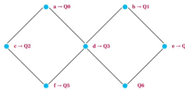
In order to illustrate the mapping steps let us consider the following circuit (see Fig. 2.3(a)) and the device’s chip layout in Fig. 2.3(c), in which circles represent the physical qubits and the edges the connections be-tween them and then possible interactions. We want to map the Gray code circuit to such as chip layout. The mapping flow that we will follow starts with a scheduler, then we set the initial placement, route and, finally, we re-schedule in order to make all the gate additions as parallel as possible. As illustrated in the dependence graph of Fig.2.3(b), there are no parallel gates. No better schedule is possible. Considering the gate times for this device the same ones as the ones described in Tab.3.2, the latency of this circuit is 400ns already.

a b ● c _● d ● e _● f _●

(a) Gray code circuit to map

a b c d e f CNOT b,a CNOT c,b CNOT d,c CNOT e,d CNOT f,e

(b) Dependence graph of the circuit

Q2 Q3 Q4

Q0

Q5

Q1

Q6 (c) Chip layout where to map the example circuit Figure 2.3: Mapping example draft

If we place the qubits based on the required interactions – that is: anext tob,bnext tocand so on – we can find in this case a placement in which all qubits can perform the required two-qubit gates as shown in Figure2.4. Then, with an optimal initial placement, we can observe that the circuit could be the same without adding any gate. No routing would be required.

b→Q2 d→Q3 f→Q4

a→Q0

c→Q5

e→Q1

Q6

Figure 2.4: Chip layout with the qubits in the optimal initial placement

However, if we do a naive initial placement in which, for instance, the virtual qubits (a,b,c . . . ) are mapped to the physical onesQ0,Q1,Q2. . . in alphabetical order (see Fig. ??). We will need to start routing them. c→Q2 d→Q3 e→Q4 a→Q0 f→Q5 b→Q1 Q6

Figure 2.5: Qubit disposition in the chip layout with a naive initial placement

2. Routing

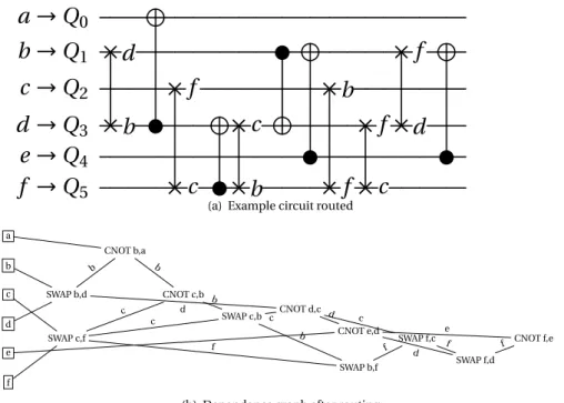
In order to allow the non-NN qubits to interact, we need to move them to adjacent positions by in-serting SWAPs. The mapping brings smartly the qubits close to the next operation qubit as well. For example, it routesbnext toabut also close toc, avoiding a path increment for the next operation. The result can be seen in Fig. 2.6(a). After every SWAP, the interchanged virtual qubits appear to follow easily the mapping. The latency after the routing increases in 1440 ns, 1440₊400=1840 ns.

2.2.Mapping of quantum circuits 9

a

→

Q

₀

b

→

Q

₁

_×

d

_●

_×

f

c

→

Q

₂

_×

f

_×

_b

d

→

Q

₃

_×

b

_●

_×

c

_×

f

_×

d

e

→

Q

₄

_●

_●

f

→

Q

₅

_×

c

_●×

b

_×

f

_×

c

(a) Example circuit routed a b c d e f SWAP b,d SWAP c,f CNOT b,a CNOT c,b SWAP c,b CNOT d,c CNOT e,d SWAP b,f SWAP f,c SWAP f,d CNOT f,e b b c b c d c d f b c f _d f f e

(b) Dependence graph after routing Figure 2.6: Naive initial placement after routing

3. Scheduling

As one could notice in the dependence graph (Fig. 2.6(b)), there are several operations that can be parallelized. Therefore, we can apply a scheduling. In the Fig.2.7the result of an ASAP scheduling is shown, reducing the latency to 1520 ns. Note that the dashed boxes enclose all the parallel operations in a cycle.

a

→

Q

₀

b

→

Q

₁

×

d

_●

×

f

c

→

Q

₂

_×

f

_×

_b

d

→

Q

₃

_×

b

_●

_×

c

_×

f

_×

d

e

→

Q

₄

_●

_●

f

→

Q

₅

_×

c

_●×

b

_×

f

_×

c

Figure 2.7: Naive initial placement routed and re-scheduled

We summarize the results of using a naive and an optimal initial placement in terms of number of gates and latency in Tab.2.3.

Table 2.3: Difference between the naive initial placement and the optimal one in terms of number of operations and latency Optimal approach Naive apprach

# operations 5 11

2.3.

State-of-the-art on the mapping of quantum circuits

Quantum algorithms are meant to leverage the promising power of quantum computers [6]. Commonly de-scribed as quantum circuits, quantum algorithms are hardware agnostic. However, as we have seen they need to be adapted – mapped – to the quantum device limitations. The main constraints in all of them is the lim-ited connectivity between qubits. There is a vast amount of literature on the algorithms – high abstraction level –, neglecting hardware constraints. From ion traps [7] to superconducting qubits [5,8], through quan-tum dots [9,10], each layout has its own requirements and constraints. Although all of them are arranged in a 2D – planar – structure, ion traps technologies are capable to connect the qubits in all-to-all networks while superconducting technologies connections form a grid shaped network where each qubit is connected to a maximum of four neighbors. This grid structure establishes one of the main connectivity limitation in today’s quantum chips, the nearest-neighbour constraint. Also industry’s superconducting chip layouts from IBM [11], Google [12] and Rigetti [13] follow this structural limitations. As for the high abstraction level of the quantum algorithm, a link between the algorithms and the devices is required [1]. As in classical computa-tion, the algorithms should go through a transformation process in order to adapt them to the hosting device. Certainly, the mapping procedure is an important element of this process.

There is a considerable amount of literature on the mapping task. Initial works on this field [14–16] focused primarily on the definition of what they characterized as aschedulerable to parallelize operations and add the required gates to route qubits. They consider general connectivity constraints as the NN one, common for most of the devices – although the works were examining ion-traps as hardware implementations. The proposed techniques by these works examine a dependency graph looking for the best way to organize qubits and operations. The majority of the methods use latency as the metric to minimize, however some of them [17] would minimize in number of SWAP operations. As it will be explained in the next section, to minimize in latency stands for time optimization while minimize in number of SWAP operations means to find the path that introduces the minimal number of SWAP operations. Following a similar reasoning as the first approaches, more complex solutions [18] have been published using Constraint Programming together with temporal planning, optimizing in latency as well. Also, several publications [19,20] outline only the routing sub-task using the number of SWAPS as the metric to minimize.

A recent review of the literature on the mapping topic focused on mapping quantum algorithms on a specific quantum device. In all the cases, taking into account the specific chip connectivity constrain. IBM’s chip have been gaining much attention due to the open online tools that make the chips accessible to everybody. Various approaches to map algorithms for the IBM family of chips have been proposed [21–24]. Zulehner et. al [21] developed a routing algorithm that optimizes in the number of SWAPs building a graph – similarly to previous works – and searching the best route in the chip layout with the A* algorithm. Siraichi et. al [22] work defines a weighted dependence graph where the mapping algorithm is able to find a solution for all the mapping steps, initial placement, scheduling and routing. Also, apart from the works related to the IBM devices, Rigetti’s devices have been approached [25].

Many attempts have been made [26–30] with the purpose of develop a FT mapping able to work at the log-ical – qubit – level. However, due to the high complexity of the QEC techniques, quantum chips with large amounts of qubits are still theory. Current and near-future quantum processors are what Preskill [31] calls Noisy Intermediate-Scale Quantum (NISQ) devices; chips with an amount of 50-100 qubits and without QEC or much simpler encodings. Several studies, for instance [32–34], have been conducted on the mapping algo-rithms required for NISQ devices. Also, the works on device specific solutions [21–25] described before, could be considered part of the NISQ works collection.

Besides latency and the number of operations that serve to analyze the quality of a mapping algorithm, few studies have been published on quantum metrics. In this thesis, we will propose another metrics to evaluate the mapping process. Fidelity has been addressed in order to characterize the error of a quantum circuit based on the qubits state [3,35]. And, recently, Quantum Volume has been defined to assert the capability of a quantum computer [36]. In the next section and in theNew metricssection we offer an overview of the important metrics in this work.

2.4.Mapping metrics 11

2.4.

Mapping metrics

As outlined in the state-of-the-art, the literature considers mainly two metrics to optimize in their mapping algorithms and as an output to evaluate how good the mapping is. These are the addedlatencyand the numberof introducedoperationsafter the mapping procedure. The routing step from the mapping process introduces SWAP gates in the quantum circuit in order to move the qubits around. And latency is the time required to run a quantum circuit in a given quantum device. It depends on the chip cycle time and thedepth of the circuit,Lat enc y=d ept h_×tc ycl e. Depth is the number of cycles the algorithm encloses. Actually, most

of the studies [14–16] assert the latency in terms of circuit depth, avoiding the cycle time specification of any device. As shwon in Fig.2.7, one can see how after some mapping process some SWAP operations have been added as well as the depth of the circuit or latency grows. From five cycles depth in the original circuit to nine cycles.

2.4.1.

Number of SWAPs

As explained before in theMapping of quantum circuitssection, routing means to introduce SWAP operations – or any other operation that allows qubits to be moved. Whenever a two-qubit gate requests two qubits that are far apart, a path in the gridlike chip layout should be given. Each step on this grid would mean a SWAP operation between the vertex qubits of that step. We already know that quantum gates are error prone and that one of the main problems that the mapping task is dealing with is to use the least amount of gates as possible. Although the general mapping problem is to avoid the introduction of error to the original algorithm, that is caused by more sources apart from the number of gates. Nonetheless, the quantum gates is one of the main error sources altogether with the decoherence time. That is the reason why the number of SWAPs is commonly used to assert the quality of a mapper, but it is not enough.

The number of SWAPs does not give any information about how long the circuit is, or how much it will be affected by decoherence. The higher number of SWAPs does not mean the longer the circuit necessarily. The SWAPs can be in parallel, for instance. It could be the case of a short circuit with a long number operation in parallel.

2.4.2.

Latency

Latency is the time required to run a quantum circuit in a given quantum device. The introduction of gates due to the mapping makes the target circuit longer. Or what is the same, the introduction of SWAPs adds several cycles to the depth of the circuit. Therefore, the latency of the circuit increases. For instance, in theMapping example, we can see how the latency grows after the circuit is routed to 1840 ns and then it is reduced to 1520 ns after re-scheduling.

One of the main source of errors in quantum computing is the decoherence, that is the quantum phenomena that makes the qubits loose their state along time. The longer a quantum device is running an algorithm, the more errors would appear. Or what is the same, the longer the circuit, the more erroneous will be the result. The task of the scheduler – one of the three mapping steps – is to look for gates that can be run in parallel. Considering that time is one of the main error sources and that the scheduler task is to make operations simultaneously, one can understand why latency is used in order to assert the quality of a mapping algorithm. Nonetheless, as the number of SWAPs this metric is not giving enough information for that.

The latency of a circuit gives an intuition of how long it is but, it is not sufficient to assess the quality of the mapping. For instance, unlike the number of SWAPs metric, it gives no information about the number of operations a circuit has.

2.4.3.

Algorithm reliability

The ideal mapping would be the one affecting the least as possible the original circuit or, what is the same, introducing the least amount of errors. Clearly, both, latency and number of SWAPs, are direct effects of the mapping procedure that have an impact in the error increase as well. To optimize in any of them stands on correct – but not sufficient – reasoning. Latency optimization assumes that the most important error source comes from the qubit lifetime. And, indeed, time is a main issue in quantum computing. Decoherence time

is not only a maximum qubit lifetime, it is harder and harder to hold a quantum state for use times closer to the decoherence time. On the other hand, to optimize in number of SWAPs stands on the intuition that the gate error is the prominent error in a quantum device. Although intuitively one can think that the more operations are in a circuit, the longer it will be; as seen in theProblem Statementsection, the higher the number of operations does not necessarily mean the longer circuit depth. Several operations can be run in parallel in the same cycle – at the same time. Actually, to minimize in latency is to maximize in parallelism. Therefore, even though related, to optimize in one or the other holds different baselines.

In addition, these metrics are not enough to assess how good the mapping process is. These metrics do not tell you how the algorithm is affected by them. In other words, will my algorithm still produce ‘good’ results after the mapping? They are related with the error rate increase but the relationship is not totally clear. For instance, it could be the case that concatenation of errors introduced by contiguous gates would end up in a correction of the first error. Or, that the busier the qubit is, the less affected by decoherence would be. In this thesis, we propose three new metrics to analyze how the mapping process affects the algorithm re-liability. As we will explain in SectionNew Mapping Metrics: algorithm reliabilitythese metrics are fidelity, probability of success and quantum volume. To perform this analysis we will map several small quantum al-gorithms on the superconducting quantum chip develop at Qutech by DiCarlo’s group [5]. In the next chapter, we will explain the constraints of this chip and the mapping model that we used.

3

Mapping on superconducting quantum

processors

In this chapter we will describe the superconducting quantum processor used in this thesis and its con-straints. Although the work done in this thesis could be apply to any quantum technology, we limit our study to the surface code 17 chip (Surface-17) developed by Leo Di Carlo’s group at QuTech [5]. In addition, we will explain the mapping model and the new metrics proposed in this work.

3.1.

Constraints of the Surface-17 chip

In this section the constraints of the superconducting Surface-17 quantum processor developed at QuTech by Di Carlo’s group are summarized. To operate on this kind of qubits, analogue signals with a specific frequency, amplitude and envelop are sent.

3.1.1.

Superconducting quantum processor architecture

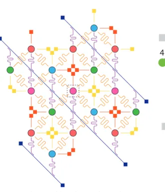
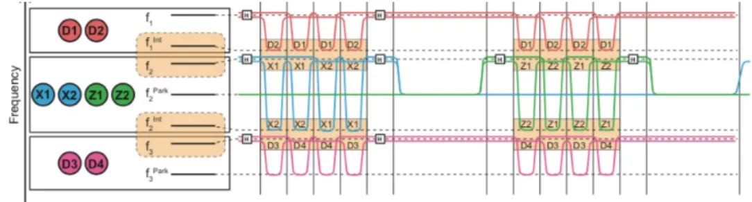
Figure3.1(a)shows a schematic of the layout for the Surface-17 chip where the circles represent the qubits [5] and the different colors the frequency used for qubit microwave control. In order to perform a single-qubit gate microwave pulses are used, whereas flux-pulses (single-qubit specific detuning sequence) are used for two-qubit gates. To this purpose, every qubit has a dedicated flux-control line (yellow) and microwave-drive line (red) to control the qubit frequency and send operating waves, respectively. Several qubits are connected through a readout resonator (in purple) to the feedlines (diagonal blue lines) that are used for measuring them. Note that readout resonators are simultaneously interrogated using frequency-division multiplexing. Finally, only qubits connected by bus resonators (in orange) can interact, this is the nearest-neighbour con-straint. For more details, please read [5].

Figures3.1(b)show a schematic of the topology for the Surface-17 quantum chip. Circles represent thequbits and theedgesrepresent the ’connections’ or possible interactions between them. Numbers are the physical addresses of the qubit. As we just mentioned the different colors represent the frequency for single-qubit microwave control: red forf1, blue and green forf2and pink forf3.

(a) Schematic of the realization of SC-17 chip [5]

0

1

2

3

4

5

6

7

8

9

10

11

12

13

14

15

16

Fe

edline 0

Fe

edline 1

Fe

edline 2

(b) Simpler layout of the SC-17. All the examples will refer to this picture Figure 3.1: SC-17 chip layouts describing its architecture

3.1.2.

Gate set, gate time and gate fidelity

In order to perform universal computation, a whole set of universal gates should be executable in a given device. However, not all kind of gates are supported in real quantum processors. In our case, any kind of single qubit rotation can be performed on the superconducting quantum processor, but gates need to be calibrated before performing any experiment and obviously one cannot calibrate infinite amount of gates. Furthermore, Z rotations do not perform very well on this kind of superconducting qubits. Based on these observations, we will limit single qubit gates to X and Y rotations, in which the most common are_±90 (degrees) and_± 180. Conditional-phase (CZ) gates and measurement in the Z basis are also possible. Therefore, the gates supported (elementary gates) by the superconducting quantum processor are:

• X gate with arbitrary angle rotation. Most common±90 and±180 degrees rotations

• Y gate with arbitrary angle rotation. Most common±90 and±180 degrees rotations

• CZ gate

• Measurement in the Z basis (M_z)

Table3.1shows the gate time and the errors rates for single-qubit gates, CZ gate and measurement [5]. Note that the default basis of measurement will be Z basis unless one specifies.

Table 3.1: The gate time and fidelity of primitive set from experiments. The measurement time includes both measuring and depletion time.

Gate type Gate time Fidelity Single-qubit 20 ns ∼99.97%

CZ 40 ns ∼99.93%

Mz 600 ns ∼99.5%

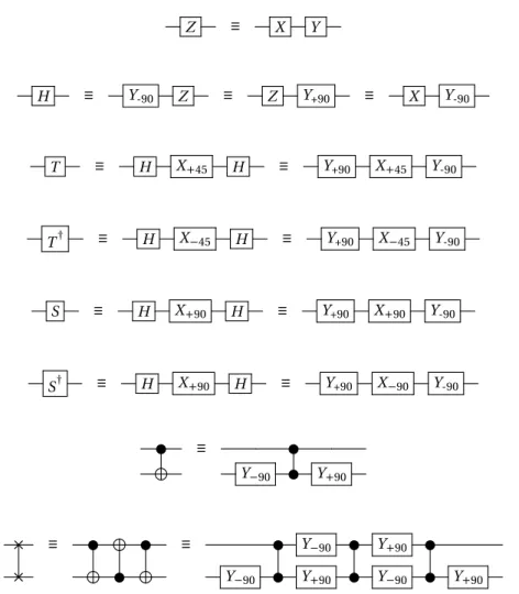
For the mapping process, we assume that arbitrary rotations and multi-qubit gates are first decomposed to the Clifford+T group, {H,T,S,CNOT}. Although this is a universal gate set that is not directly supported by the quantum chip. These gates need to be further decomposed into the elementary gates as shown in Figure3.2.

3.1.Constraints of the Surface-17 chip 15 Z ≡ X Y H ≡ Y-90 Z ≡ Z Y+90 ≡ X Y-90 T ≡ H X₊45 H ≡ Y+90 X+45 Y-90 T† ≡ H X₋45 H ≡ Y+90 X−45 Y-90 S ≡ _H X₊90 H ≡ Y+90 X+90 Y-90 S† ≡ _H X₊₉₀ H ≡ Y₊₉₀ X₋₉₀ Y_-90 ● ≡ _● Y₋90 ● Y+90 × ≡ _{● ●} ≡ _● Y₋90 ● Y+90 ● × ● Y−90 ● Y+90 ● Y−90 ● Y+90

Figure 3.2: Decomposition in the X-Y-Z-CZ set of the Clifford + T gates that are not directly supported in the quantum chip

Their gate time – shown in Table3.2– depends on the gate time of the gates in which is decomposed. We show this gate times, the gate time of the chip allowed gates, in Table3.3.

Table 3.2: The gate time for the universal set {H,S,T,CNOT}.

Gate type Gate time

X 20 ns Y 20 ns Z 40 ns H 40 ns S/Sdag 60 ns T/Tdag 60 ns CNOT 80 ns SWAP 200 ns MZ 600 ns

Table 3.3: The gate time for the universal set allowed in the devices{RX,RY,C Z,MZ}

.

Gate type Gate time

RX(±45,±90) 20 ns RY(±45,±90) 20 ns

CZ 40 ns

In the next sections, the different constraints of the superconducting quantum chip will be explained in detail. Note that we will distinguish two kind of constraints: the ones coming from the quantum chip- e.g. nearest-neighbour interactions- that we callhardware constraintsand the ones from the electronics control setup -e.g. qubits operated by the same AWG- calledelectronics constraints.

3.1.3.

Qubits interaction constraint

In Surface-17 each qubit is connected to a maximum of four qubits, the nearest-neighbours, limiting the possible interactions -e.g. two-qubit gate- between them (hardware constraint). This constraint will make that qubits that need to interact and are not place in neighboring positions will need to be moved to adjacent positions. Quantum states in superconducting technology can be ‘moved’ by using SWAP operations. This constraint implies that in Surface-17 (see Figure3.1(b))

It is possible to do:

1 CZ q[1],q[5] 2 CZ q[8],q[6]

but impossible to do (directly, without any map-ping):

1 CZ q[1],q[2] 2 CZ q[0],q[16]

The code shown here and in the next sections is written in an eQASM fashion. The letters represent the kind of gate operation and the number will refer to the qubit number in the Surface-17 layout (Figure3.1(b)). Also, the character ’|’ represents the operations that can be executed in parallel.

3.1.4.

Frequency constraint

Single-qubit gates

In order to perform single-qubit gates, electromagnetic microwaves are sent. As shown in Figures3.1(b), three or four different frequencies for single-qubit microwave control can be used in Surface-17. In principle, any qubit can be operated individually and then any combination of single-qubit gates can be performed in parallel. However, qubits using the same frequency are controlled by the same Quantum Waveform Generator (QWG) and then they are limiting the possible parallelism of operations.

Table 3.4: Frequency groups for Surface-17 when using 3 different frequencies.

QWG Qubits Frequency Group

0 1, 2, 3, 13, 14, 15 f1

1 7, 8, 9 f3

3.1.Constraints of the Surface-17 chip 17 It is not possible to perform two different single-qubit gates at the same time on qubits using the same fre-quency and operated by the same QWG. For instance in SC-17,

It is possible to do: 1 { X q[1]|X q[7] } 2 8{ X q[6]|Y q[7] } 3 { X q[1]|X q[2]|X q[5]|X q[0] } 4 { Y q[10]|Y q[4] } But not 1 { X q[1]|Y q[2] } 2 { X q[5]|Y q[0] } 3 { X q[10]|Y q[4] } 4 { X q[7]|Y q[9] }

Obviously, it is not possible to perform more than one single-qubit gate on the same qubit at the same time (gate dependency).

Two-qubit gates

In order to perform a two-quibt gate in superconducting qubits, interacting qubits need to be brought to a specific close frequencies [5]. More specifically,C Zf gates are performed between qubits atf

i nt

1 andf2or at

f2i nt andf3as shown in Figure3.3. In addition, the qubits that share a connection with the qubits performing a 2-qubit gate need to be detunned away. This limits the amount of two-qubit gates that can be performed in parallel (hardware constraint).

Figure 3.3: Frequency arrangement and detuning frequencies for the qubits in the unit cell.

As we assume the frequency scheme of Figure3.3we can formulate the following: 1) If a two-qubit gate is being performed between D1 (D2) and X1 (X1 or Z1), D2 (D1) cannot interact with X1 or Z1 (X1) at the same time; 2) In the same way, if a two-qubit gate is being performed between D3 (D4) and X1 or Z2 (X1 or Z1 or X2 or Z2), D4 (D3) cannot interact with X1 or Z1 or X2 or Z2 (X1 or Z2) at the same time. Obviously, if a two-qubit gate is being performed between two qubits, the qubits involved can not perform another single-or two-qubit gate at the same time.

As an example, in Figure3.4, a CZ gate is applied between qubits 11 and 14 (cz (q[11], q[14])). Thus, both qubits need to be tuned to closer frequencies –f1i nt andf2in this case. And, as explained before, in order to not create intereferences between qubits some of them should be detunned away. Specifically, qubits 10 and 16 need to be detunned to f₂par k because they share a connection with the qubits performing the CZ gate. This means that no single-qubit gate can be applied to these qubits that are outside their main frequency (f2). And, also, that they cannot perform another two-qubit gate at the same time with any other qubit from the QWG 0 – the red qubits with main frequencyf1– because it is required to tune them tof2.

Finally, all the qubits that are already in use cannot be used at the same time. Therefore, qubits 11 and 14 in the example cannot be used in any single- or two-qubit gates.

3.1.5.

Measurement constraint

Measuring the qubits is done by using feedlines coupled to several qubits. For example, in the SC-17 chip, the feedline 1 is used to measure qubits 1, 4, 5, 7, 8, 10, 11, 14 and 15. This will lead us to the last limitation, the

measurement constraint(hardware constraint). In this case, the measurement on a qubit cannot start when

another qubit coupled to the same feedline is being measured, but it allows to start measurement on any combination of qubits coupled to the same feedline at the same time. Furthermore, there is no dependency between measurements of any two qubits coupled to different feedlines.

0

1

2

3

4

5

6

7

8

9

10

11

12

13

14

15

16

Not allowed interactions CZ gate Not-allowed qubit for

single-qubit gate

Figure 3.4: Example of a two qubit gate and allowed and not allowed parallel gates in SC-17

In SC-17, it is possible to do

1 measure q[0]|measure q[2] |measure q[3]|measure

q[6]|measure q[9]| measure q[12]

↪

2 measure q[1]|measure q[13]

3 qwait30

4 measure q[3]|measure q[8]

notice that the measurement of qubits 13 and 16 is executed at the same cycle.

On the other hand it is not possible to do

1 measure q[2]

2 measure q[6]

Note that, in order to measure qubit 2 and 6 in different times, the latter instruction should wait 30 cycles for the first one to finish. In other words, this code is missing aqwait 30 instruc-tion.

3.2.

Mapping model

In order to map quantum circuits on the superconducting quantum chip we will use the mapping model developed in our group [30]. A mapping algorithm or mapper is an algorithm able to find a mapping solu-tion given a quantum circuit and a target device. We consider that a mapper is subdivided in three tasks: scheduler, initial placement and routing, as described in theMapping of quantum circuitssection. Our pro-cedure is modular, although the flow is restricted to the one described below. The mapper is fully adaptable to any device constrain. As we will explain, it also offers two different kinds of schedulers and three router possibilities, as well as the option of running or not the initial placement and another options related to the chip constrains. We believe this solution will aid researchers to investigate the best mapping, with different configurations. The mapping model works as follows.

3.3.New Mapping Metrics: algorithm’s reliability 19

3.2.1.

Initial placement

The first step is to map the virtual qubits (the ones of the circuit) to the physical ones (the ones in the quantum chip). Once the mapper knows the qubits required by the algorithm, it will try to find the best initial place-ment for the given circuit, that is, the placeplace-ment that requires less moveplace-ments of qubits. First, it will check the first set of two-qubit gates and their target qubits. If those qubits are not NN, it will initiate an Integer Liner Programming (ILP) algorithm [30] to find the optimal initial placement. This optimal initial placement tries to place the qubits in a way that the minimum number of qubit movements are required.

3.2.2.

Router

The function of the router is to move non-neighbouring qubits to adjacent positions whenever they need to interact. To this purpose, our router inspects all the gates, one by one, looking for non-NN qubits interactions. Whenever the router encounters one, it will calculate several shortest paths – the ones that use the minimal amount of SWAPs – and selects one of them. This path is selected based on the circuit depth, that is, the path that better interleaves with the previous operations. Then, it will insert the SWAP operations (decomposed or not decomposed) required to follow the selected path.

There are three router options, and a different path is selected depending on the router option that was se-lected by the user:

1. basefinds all the shortest paths and selects one of them randomly. The shortest paths are calculated based on the Manhattan distance, counting the number of steps that the qubits will need to move. 2. minextendfinds all the shortest paths as well, but selects the one that will minimally increase the

circuit depth. In this case, only gate dependencies are considered, not chip constraints that limits the parallelism.

3. Theminextendrcapproach is exactly the same as the second one, but taking into account the chip constraints when selecting the path.

3.2.3.

Scheduler

The RC-scheduler will finally schedule the circuit using either an ALAP or an ASAP approach, depending on the user requirements. It will take into account the chip parallelism constraints, as the ones described in3.1. One downside factor regarding this methodology is that the mapper only takes into account one gate every time. It does not look ahead in order to decide the best path for next iterations. Or, what is the same, it does not always find the best mapping solution. This limitation comes from the fact that, the more steps you are looking ahead while mapping, the more computationally complex will the mapper be. We highlight that the mapping problem is an NP problem [22]. Therefore, this method represents a viable solution, although a lot of future work should be done.

3.3.

New Mapping Metrics: algorithm’s reliability

As mentioned in theMapping metricssection in the second chapter, we namemapping metricsto those met-rics used to assert the quality of a mapper and that are also used by the mapper algorithm as a cost function to optimize. In this section, we will present and define some new mapping metrics:fidelity,probability of successandQuantum Volume.

3.3.1.

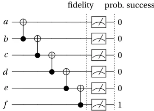
Fidelity and Probability of success

Fidelity and probability of success are two different ways to measure how errors affect the algorithm reliability. Fidelity is measured before measuring the qubits, and it is the difference between the obtained quantum state (affected by errors) and the expected quantum state (the one without errors). Probability of success is obtained after measuring the qubits, and then after collapsing the quantum state. Note that in this case measurement errors are also considered. After running the algorithm several times, it shows how many times

fidelity prob. success a 0 b

●

●

●

_●

_●

Figure 3.5: Example of the fidelity and probability of success calculation in the Gray encoder quantum circuit

a correct result is measured. Therefore, while fidelity is a theoretical metric that can only be calculated in simulations, the probability of success is a hardware metric that can be asserted in experiments in real life.

Fidelity

Fidelity compares two quantum states. Unlike the success of an algorithm, that is a boolean metric – either success or failure –, the fidelity returns a float number between 0 to 1 asserting how different the states are – how far is one state from the other. 0 fidelity would mean that the states are the same – they do not differ – and 1 would mean that states are perpendicularly different. As an analogy, if we consider the quantum states as vectors, the fidelity would be the dot product between them. However, the fidelity between orthogonal states – states that differ in rotations around the x-axis as∣0100⟩,∣0001⟩and∣1111⟩– is also 0. For more information, we refer to [3].

Probability of success

We define probability of success as the probability of having the correct or expected results after running and measuring several times a quantum algorithm. For instance, if the expected result of an algorithm is0100 and the results are either0001or1111we will get a failure. We will only get a success if the algorithm returns 0100. Then, in the previous example, if we get0001,0100and1111as results after running the algorithm three times the resulting probability of success will be1₃.

In our study, we will use both metrics in order to study how the mapping process and then the amount of errors affect the algorithm reliability. Note that as we already mention, the fidelity is calculated before mea-surement and then it does not take into account the meamea-surement errors. It could be the case that a quantum state is erroneous before the measurement and, then, due to the error added from the measurement the erro-neous state would flip and converge into the expected state. At the same time, a correct quantum state could be measured wrongly due to the measurement errors.

It is worth noting that both metrics, the fidelity and probability of success, are obtained by using a quantum computer simulator as we will explain in the next chapter.

3.3.2.

Quantum Volume

Another metric that could be useful for the mapping quality assessment is Quantum Volume [36,37]. Quan-tum Volume is a metric proposed by IBM to depict whether a device is able to run a quanQuan-tum circuit or not. Given the different hardware implementations and technologies in Quantum Computation (superconduct-ing, ion-trap, spin qubits, . . . ), it is often difficult to benchmark the usefulness or power of quantum systems. The aim of Quantum Volume is to quantify the computational power of quantum devices. Consequently we will use it as a metric to measure the runnability of the quantum algorithms on the quantum devices. But, while the device is the target of the Quantum Volume metric, we focus on the circuit. Our goal is to assess how the mapping procedure affects the runnability of a given circuit and to study how the Quantum Volume is related to the fidelity and the probability of success.

The general Quantum Volume formula is defined in eq. 3.1whereN is the number of physical qubits and

3.3.New Mapping Metrics: algorithm’s reliability 21 some device, are correctable and useful. d(N)depends on the number of qubits in the circuit as well as on the error rate of the quantum device.

V_Q=min(N,d(N))2 (3.1)

In our case, we want to relate the Quantum Volume of a device with the circuit. Therefore, we define the algorithms Quantum Volumeand therunnabilityof the quantum circuit on a given device.

As withVQ, we initially derived the algorithm’s Quantum Volume from the general equationVQ(see eq.3.2),

although we will adapt it later.

VQa=min[n,d] 2

(3.2) Note thatdis notd(N)but the real depth of the given algorithm. At the same time,nis the number of qubits required by the algorithm itself.

We are aware that this approach has a limitation regarding the mapping of the quantum circuit. As explained before,VQ is able to take into account the sophistication of the mapping procedure. It is inherited in the

model algorithm. But, in this case, theV_Qaof an algorithm before and after mapping will remain the same.

After mapping an algorithm, the usual effect is an increase in the depth and the number of operations. Rare mapping methods consider the qubit addition in the technique. And, even considering it, n is not often growing too much in comparison withd. In the current NISQ era, the quantum circuits need much less qubits than depth. Therefore, most of the times, the minimum value betweennanddwill ben. As soon asV_Qais taking into account the minimum of them and the mapping procedure affects mostly tod we can conclude that this definition ofVQais not considering the mapping in its results.

A simplified solution for this problem would be theV_Qadefinition as the multiplication betweennandd(see eq. 3.3). Unfortunately, this approach has several drawbacks as well. As Moll et al. point out [36], extreme cases of highnand lowd– or the other way around – lead to inconsistencies of the multiplication metric. But, considering that most of our work is not going to be in any of these extreme cases and that we can avoid those outliers, we define the algorithm’s Quantum Volume as:

VQa=n×d (3.3)

Finally, once the Quantum Volume of an algorithm is stated, we define runnability as the condition for which theVQshould be bigger thanV

a

Q. That is the condition that the computational power of the device should be

bigger than the computational power required by the algorithm.

Runnable if:VQ>VQa whenN≥n (3.4)

For instance, in order to understand this concept, one may imagine the process of checking, whether or not, some cube with a given volume – representing the algorithm – would fit in a box – the device –. If the algorithm’s box volume is smaller than the volume of the device’s box, the algorithm’s box will fit inside. Indeed, one acceptable criticism of this definition is that, asVQ andVQaare finally defined in the previous

sections, it seems that it is not really fair to compare them. But, as soon as the general behaviour of both def-initions ofVQais the same we believe that this definition of runnability is mathematically correct and useful.

4

Benchmarks and analysis framework

In this chapter we describe the benchmarks that will be mapped to the Surface-17 chip and the simulation framework develop for the study of the mapping metrics.

4.1.

Benchmarks

In order to analyze the different metrics to assess the quality of a mapping algorithm, we selected a set of quantum algorithms available in the literature.

I built a list of quantum algorithms coming from different sources. The sources we chose are RevLib [38], ScaffCC [39], some benchmarks from Zulehner’s et al. work [21] and QLib [40] because of the variety of al-gorithms and because they are already decomposed in the Clifford+T set. Note that the language used to describe the algorithm varies from source to source. Although, they all use a QASM-based language, there are small syntax differences. As we will explain in the next section, we will use our own programming languages – OpenQL and cQASM – and compiler. Therefore we had to translate all the selected algorithms from their QASM versions to the OpenQL notation. I developed a parser in order to do that.

I also profiled each benchmark including: the number of qubits of the algorithm, the number of gates, the functionality of the algorithm and different graphs, showing the percentage of the operations types or the degree of parallelism of the algorithm. Most of the benchmarks are classical algorithms adapted to quantum circuits. They are deterministic and then the result is always the same if there are no errors. This is because at the end of the circuit, before measuring the qubits, qubits are in either ground or excited state, but never superposition.

The benchmarks were also classified by their functionality. This is an important step because algorithms that do similar calculations use to have common gates distribution. From all the benchmarks we have, we can distinguish six different classes.

• Quantum Gates: Circuits that are a decomposition of a Quantum Gate

• Search Algorithms

• Worst Cases: Circuits that were really difficult to generate for RevLib

– HWB: is the simplest function with exponential Ordered Binary Decision Diagrams (OBDD) size.

• Encoding Functions: Classical codification functions

• Arithmetic Functions: Functions that perform an arithmetic operation

• Miscellaneous: Mix of different kind of algorithms

We came up with a list of 84 different algorithms – 697 benchmarks taking into account the different versions of the same functionality – that can be found in theqbench Github repo, as well as the previous information

in much more detail. These algorithms cannot only be used for the mapping problem but also for other activities in our group.

4.1.1.

Benchmark selection

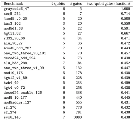
In order to have a small, but representative, set of benchmarks to map, we selected just some of them. This requirement comes by the fact that simulations are long and computationally exhaustive. In order to do that, we studied the different benchmark profiles looking for most illustrative cases. The criteria used for selecting the algorithms used in this work are: i) the number of qubits of the algorithm. It should be less than 17 as we will use the Surface-17 chip; ii) the number of gates. We select benchmarks with a number of gates as spread as possible; iii) different functionality. We try to have the least number of versions of the same algorithm as possible. We only take the same algorithm versions for cases in which the number of qubits and the number of gates show an interesting combination. For example, two similar algorithms in which number of qubits or number of gates are very distinct appear as the first three selected benchmarks in Tab.5.1.

Once we had our requirements we could start the analysis and the selection afterwards. In Tab.5.1we show the final benchmark selection. 43 benchmarks (with qubits numbers from 3 to 17 qubits) were selected after Table 4.1: Restriction summary of the benchmark selection

Criteria: - # qubits < 17

- # gates as spread as possible and in the case of repeated benchmark the minimum number of gates - The less number of the same algorithm versions/classes as possible

- The benchmarks that are repeated and have an interesting combination of No. qubits/No. gates are preferred

applying the previous restrictions to the analysis of the benchmarks described in the next section (see Table

5.1). After simulating the algorithms, few of them returned errors (segmentation fault) due to the high com-putational level they required and some others did not finish the simulation in less than two weeks; so we discarded them.

4.2.

Analysis framework

In this section we introduce the framework used to map the quantum algorithms and analyze the quantum metrics. It is based on two steps: compilationandsimulation. With this purpose we connect two tools, OpenQL [41] and quantumsim [4], and we build a whole framework over them.

4.2.1.

Compiler (OpenQL)

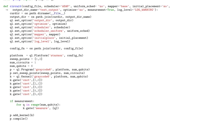
OpenQL is a framework for high-level quantum programming developed by our group to describe quantum algorithms and compile them. The framework can be found as a library in either C++ or Python and, there-fore, the circuits are described over one of these programming languages. It can target real quantum chips as well as different quantum computer simulators such are QX simulator [42] or quantumsim [4].

One of the passes of the compiler is themapperalgorithm developed by our group. It performs the initial placement, schedule the operations and route the qubits taking into account the quantum chip constraints that are described in a JSON file. It is also able to load different compiler configurations like the kind of scheduler, router or initial placement. We will use OpenQL to describe the selected benchmarks and compile them for the SC-17 chip. In Fig. 4.1we show an example of OpenQL code using Python that describes the Gray encoder quantum circuit (Fig.2.2). More insights can be found in thegithub repository.