Quantum phase transitions and quantum transport in low-dimensional topological systems

(1)

QUANTUM PHASE TRANSITIONS AND QUANTUM TRANSPORT IN LOW-DIMENSIONAL TOPOLOGICAL SYSTEMS

by

BARI ¸S PEKERTEN

Submitted to the Graduate School of Engineering and Natural Sciences in partial fulfillment of

the requirements for the degree of Doctor of Philosophy

Sabancı University June 2017

(2)

APPROVED BY

Assoc. Prof. ˙Inanç Adagideli ... (Thesis Supervisor)

Assoc. Prof. Emrah Kalemci ...

Assoc. Prof. ˙Ibrahim Burç Mısırlıo˘glu ...

Assoc. Prof. Özgür Esat Müstecaplıo˘glu ...

Assoc. Prof. Levent Suba¸sı ...

(3)

c

(4)

ABSTRACT

Barı¸s Pekerten Ph.D. Thesis, June 2017

Thesis Supervisor: Assoc. Prof. ˙Inanç Adagideli

Keywords: Mesoscopic and nanoscale systems, topological insulators and superconductors, random matrices, spintronics, quantum thermodynamics

In this thesis, we focus on quantum phase transitions that change the topological index of topological insulators and superconductors, which are states of matter featuring topo-logically protected edge states and insulating bulk, and on transport of charge and spin in topological insulator nanostructures. We consider topological phases in disordered quasi-1D topological superconductors. The Majorana edge states on topologically nontrivial nanowires were previously found to be protected from disorder as long as the localization length is larger than the coherence length, after which the wire transitions to a trivial state. We find that changing disorder can push the system back into a topological state in mul-tichanneled nanowires, creating previously unreported fragmentation of the topological phase diagram. We next discuss arbitrarily-shaped and/or disordered topological super-conductors and their ground state fermion parity. As external parameters are varied, even and odd parity ground states cross, causing quantum phase transitions. We find that the statistics of parity-crossings are universal and described by normal-state properties and determine the shape dependence of the parity crossings. Finally, we consider edge state quantum transport in quantum spin Hall insulators in the presence of nuclear spins. We find that a properly initialized nuclear spin bath can be used as a non-energetic resource to induce charge current in the device, providing power an external load using heat from electrical reservoirs. Resetting the spin-resource requires dissipation of heat in agreement with the Landauer’s principle. Our calculations show that the equivalent energy/power density stored in the device exceeds existing supercapacitors.

(5)

ÖZET

DÜ ¸SÜK BOYUTLU TOPOLOJ˙IK S˙ISTEMLERDE KUANTUM FAZ GEÇ˙I ¸SLER˙I VE KUANTUM TA ¸SINIM

Barı¸s Pekerten Doktora Tezi, Haziran 2017 Tez Danı¸smanı: Doç. Dr. ˙Inanç Adagideli

Anahtar kelimeler:Meso ve nanoölçekli sistemler, topolojik yalıtkan ve üstüniletkenler, rastlantısal matrisler, spintronik, kuantum termodinami˘gi

Bu tezde, maddenin topolojik olarak korunumlu kenar durumları ve yalıtkan yı˘gın içeren bir hali olan topolojik yalıtkan ve üstüniletkenlerin topolojik indisini de˘gi¸stiren kuantum faz geçi¸slerine ve topolojik yalıtkan nanoyapılarda yük ve spin ta¸sınımına odaklanıyoruz. Öncelikle düzensiz, bir boyutlumsu topolojik üstüniletkenlerde topolojik evreleri ele aldık. Daha önceden topolojik açıdan sıradı¸sı evreli bir nanokablodaki Ma-jorana durumlarının yerelle¸sme mesafesinin e¸sevrelilik mesafesini a¸stı˘gı sürece düzen-sizli˘ge kar¸sı korunumlu oldu˘gu bulunmu¸stu; bu düzensizlik seviyesinden sonra kablo, sıradan evreye geçer. Biz ise bundan daha da fazla düzensizli˘gin çok kanallı nanokablo-ları topolojik evreye geri zorladı˘gını ve topolojik evre çizgesini daha önce gösterilme-mi¸s bir ¸sekilde parçaladı˘gını gösterdik. Devamında geli¸sigüzel ¸sekilli ve/veya düzen-siz topolojik üstüniletkenleri ve taban hal fermiyon e¸sli˘gini tartı¸stık. Harici de˘gi¸skenler de˘gi¸stirildikçe tek ve çift pariteli taban durumları kesi¸sir ve kuantum evre geçi¸sine sebep olur. Biz bu parite kesi¸sim istatisti˘ginin evrensel odu˘gunu ve bu istatisti˘gin normal durum özellikleriyle belirlendi˘gini gösterdik. Ayrıca parite kesi¸simlerinin ¸sekil ba˘gımlılı˘gını da ifade ettik. Son olarak çekirdek spinleri varlı˘gında kuantum spin Hall yalıtkanının ke-nar durumunun ta¸sınım özelliklerini ele aldık. Uygun ¸sekilde hazırlanan bir çekirdek spin banyosunun enerjisiz kaynak olarak kullanılıp sistemde bir yük akımı tetiklemek için kul-lanılabilece˘gini ve bu akımın elektrik rezervuarlarının ısısını kullanıp harici bir dirençten güç açı˘ga çıkarabilece˘gini gösterdik. Spin kayna˘gını sıfırlamanın Landauer prensipine uygun olarak ısı yayılımı gerektirdi˘gini gösterdik. Hesaplarımız, sistemde depolanan e¸sde˘ger enerji/güç yo˘gunlu˘gunun halihazırdaki süperkapasitörlerin yo˘gunlu˘gunu a¸stı˘gını göstermektedir.

(6)

ACKNOWLEDGEMENTS

The author of this thesis would like to declare his deep love for and indebtedness to his family, who have been supportive of him throughout thick and thin. The process of obtaining this Ph.D. was no different: There was the thick, and there was the thin; and there his family was, as always.

The author would also like to convey his heartfelt gratitude to his supervisor, Dr. ˙Inanç Adagideli, for the many years he patiently taught and guided the author. The author would also like to communicate his thanks to his co-authors for an excellent research environment.

The author would like to express gratitude to The Science Academy (Bilim Akademisi) Turkey and to Feza Gürsey Center for Physics and Mathematics for the use of their fa-cilities. The author also gratefully acknowledges financial support from the Erdal ˙Inönü chair, from Scientific and Research Council of Turkey (TUBITAK) through their Scien-tist Support Program (B˙IDEB) scholarships, from Lockheed Martin Corporation Research Grant and from COST Action MP1209.

(7)

List of Figures and Tables

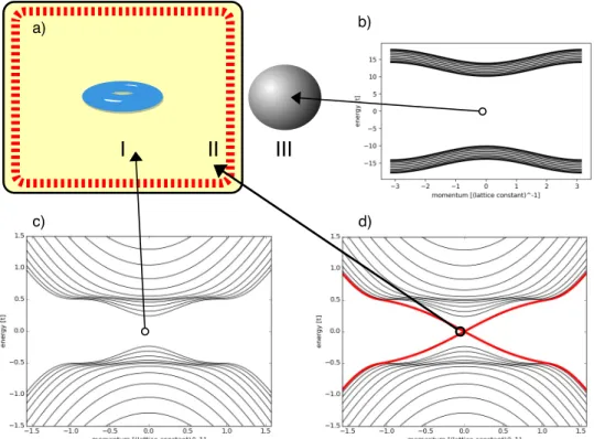
2.1 A schematic picture of a topological insulator in two dimensions. The yel-low shaded structure in (a) is the topologically nontrivial material, with the torus representing the topology of the mapping between its Hamilto-nian and an appropriate Bloch sphere over the Brillouin zone. The similar mapping from vacuum has a trivial topological shape of a sphere. The band structure of the discretized system in the tight binding model is given for the bulk in (c), for the edges in (d) and for the surroundings in (b). The bulk boundary correspondence forces the gap to be closed and a gapless edge state to be formed (the red band in (d) ). . . 5 2.2 A schematic picture of a wavefunction_|ψ(ξ)_i, represented by the arrows,

that depends on some parameter vectorξ. We are interested in what hap-pens to the phase of_|ψ(ξ)_ias the parameter is changed on a closed curve Cξ. . . 7

2.3 A sphere in the d(k)-space, separated into two hemispheres. At each point on this sphere, the eigenkets_|n_iare defined. One of the hemispheres contains a point on which the curl of the_|n_i“vector” is not well defined. Within each hemisphere, _|n_i is smooth along the boundary, but as one goes across a boundary, a discontinuity presents itself in the phase of_|n_i. 11 2.4 The Haldane model, with a staggered onsite energy_±∆, nearest neighbor

t1 and next-nearest neighbort2eiφhopping on a honeycomb lattice. . . 13

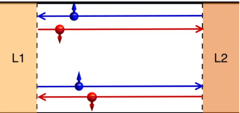
2.5 A quantum spin Hall insulator in 2D, with external attached leads L1 and L2. In this subsection, we usually consider closed systems, but we consider open systems with leads later. At each edge, a spin-polarized current flows: On the bottom edge, spin-down electrons move left and spin up electrons move right. The opposite is true for the top edge. . . 14

(11)

2.6 Example band structure of a _Z2 topological insulator. (a) Band

struc-ture of a HgCdTe wire, using realistic parameters (see Table 2.7) but dis-cretized on a square lattice of side a = lSO/40. The lattice is 20a wide and infinitely long. t = _~2/2ma2 is the hopping parameter. The grey bands are the bulk bands and the red bands are the edge modes. If the Fermi level is held at the dashed line, the system will support topologi-cally protected spin polarized edge modes. (b) Between the two Kramers degenerate points k = 0 and k = π, the Fermi level crosses the edge states an even number of times. Hence, this system is not topologically protected. (c) The Fermi level crosses the edge modes an odd number of times, thus the system is topologically nontrivial. . . 16 2.7 Material parameters for a HgCdTe quantum well for two different

thick-nessesdof the QW. In the second row,M/B >0and the system is in the nontrivial state [32]. . . 16 2.8 A Kitaev chain of N sites. (a) Each fermion on the site can be divided into

a real and an imaginary part, each a Majorana fermion. (b) The Hamil-tonian, when diagonalized, couples Majorana fermions of different sites, leaving a pair uncoupled, each one at a different end. . . 21 2.9 The periodic table of topological insulators, adapted from [34], listed with

respect to their Altland-Zirnbauer classification and the presence or ab-sence of a time reversal (Θ), particle-hole (Ξ) or chiral (Π) symmetry. The right side of the table lists the type of the topological invariant, if any. The table repeats itself from d tod+ 8, in what is called the Bott periodicity [68]. . . 28 2.10 The constraints on theS-matrix depending on the Altland-Zirnbauer class

in 1D. Only topologically nontrivial phases are shown. The first row rep-resents the AZ class, the second row gives the group of the topological phase, the third through fifth rows give the constraint on the S-matrix that the presence of the relevant antiunitary symmetry imposes (0means the system does not have that symmetry). The SR symmetry row is for the presence or absence of the spin rotation symmetry in a given system. The second-to-last row gives all the constraints on the reflection matrix, whereas the last row shows how to obtain the topological quantum num-ber_Qfrom a givenS (indeed,r) matrix. ν(r)is the number of negative eigenvalues ofr. Adapted from [69]. . . 30

(12)

2.11 The wire and its ending considered by Fulgaet al.[69] in their derivation of the topological numbers from the properties of theS-matrix. . . 31 3.1 The multichanneled nanowire of widthW,which is an RSW topological

superconductor with a Gaussian disorder having an average value_hV_i= 0. (a) In the leads, we takeαSO, ∆ andV(x, y) to be zero, making the leads metallic. Our analytical results assume a semi-infinite wire (L _→ ∞), whereas in our numerical full tight-binding calculations we use wires of length L lMFP, ξ, lSO. (b) The form of the wire used to construct the Majorana solutions in section 3.2.1. The part of the wire left of the scattering region is again metallic. . . 35 3.2 µvs. B vs. QD for a five-channel system (compare with Figs. E.4 and

E.3.) The background red-white colors are obtained using a numerical tight-binding simulation withL = 30000aandW = 5a, while the black lines, which represent the topological phase boundaries, are obtained an-alytically using Eq. (3.7). Here,V0 =

p

γ/a2 _{= 0}_.₂_t, _α

SO = 0.02~/ma (lSO = 4.08µm) and∆ = 0.164t, wheret=~2/2ma2 anda= 0.01lSO is the tight-binding lattice spacing. The fragmented nature of the topolog-ical phase diagram seen in (b) cannot be explained in a p-wave picture. See Appendix D for a discussion of corresponding experimental parameters. 41 3.3 µ vs. V0 =

p

γ/a2 _vs. _Q _{for a multichannel RSW wire. The black}

lines, which represent topological phase boundaries, are obtained ana-lytically using Eq. (3.7). The background red-white colors are obtained using tight-binding numerical simulations with L = 60000a. In both cases, W = 4a, αSO = 0.015~/ma, ∆ = 0.20t and B = 0.35t, where t = _~2/2ma2 is the tight-binding hopping parameter and a is the TB lattice spacing. See Appendix D for a discussion of corresponding exper-imental parameters. . . 42

(13)

4.1 A plot of the lowest ten eigenvalues of the disordereds-wave Hamiltonian in Eq. 4.11, discretized on a 1D lattice of 100 sites, plotted as a function of (a)B/t and (b)√B2₋_∆2_{/t, for different values of Hamiltonian}

pa-rameters. In both plots, the black set of curves represents the lowest ten eigenvalues obtained for∆ = 0.5t, α = 0.08ta,µ = 2.0t; the red set is for ∆ = 1.4t, α = 0.04ta, µ = 2.298t; the green set is for ∆ = 1.8t, α = 0.05t, µ = 2.0t; and the blue set is for ∆ = 1.8t, α = 0.1ta, µ= 1.6t. Here,t = _~2/2ma2 is the hopping parameter. In all cases, the disorder strength is the same. Of interest is the statistics of each eigen-value crossing the zero point. (Particle-hole symmetry assures another state will cross zero at the same point; level repulsion does not occur be-cause of this symmetry.) Note that when the same plot in (a) is plotted as a function of√B2₋_∆2_{, all crossings happen at the same points for all}

parameters. . . 49 4.2 Level spacing distributions for localized wire with (a) L `, (b)L_& `

and (c) L _. ` in the p-wave regime. The red lines correspond to the Poisson distribution (Eq.Z4.9), the green line is semi-Poissonian (Eq 4.10 and the red line is Wigner-Dyson (Eq. 4.8). As the system becomes less polarized, an opposite spin comes into the picture ((e) through (f)), the statistics start to involve two independent sequences of crossing spaces even though each sequence is correlated within itself. Thus, the level repulsion disappears, while the large spacing tail remains Gaussian. . . . 50 5.1 The quantum spin Hall insulator with nuclear spins and electron-nuclear

spin flip interaction. (a) The band structure of a typical QSHE nanowire system (using the BHZ model with tight-binding approximation). Red lines represent the edge states. (b) The band structure of the simpli-fied Hamiltonian heff projected to a single edge (dashed blue lines). (c) Schematic description of the QSHE system with the edge currents inter-acting with the nuclear spins in the system, with the diamonds represent-ing nuclear spins. (d) The spin flip interaction with the nuclear spins that form the Maxwell Demon. . . 56

(14)

5.2 (a) QSH based quantum information engine, providing power to loads 1 and 2. Schematic description of (b) the charging and (c) the discharging phase of the QIE. In the charging phase, an applied bias current aligns the nuclear spins. In the discharging phase, flipping nuclear spins drive a current. An applied reverse bias can extract power. . . 59 5.3 P-V graph, calculated using Eq. 5.11, (a) as a function of mean

polariza-tionmwithζ = 1.0and (b) as a function ofζ with full polarization m = 0.5. On the dashed line, P = 0. Power can have negative values forV <0 (V >0)for a given mean polarizationm > 0 (m < 0)(here, e > 0), as an indication of the work extraction phase. . . 60 A.1 The orbits of electrons in a quantum Hall system under an applied

mag-netic field. The closed cyclotron orbits form the Landau levels. At the edges, a chiral state travels in a single direction, determined by the di-rection of the magnetic field B. These “skipping orbits” in this cartoon picture are shown in red. . . 83 A.2 The QHE cylinder used by Laughlin to make his argument. A magnetic

field pierces the sides of the cylinder in a perpendicular fashion. Current is applied around the sides, and a Hall voltage VH is observed. Under

sufficiently strong magnetic fields, the conductanceI/VH is quantized as

a function of magnetic field. . . 84 A.3 qunit cells of sizea_×b, admitting a total ofpflux quantaφ0. Ifpandq

are mutually prime, then this figure depicts a magnetic unit cell. . . 86 A.4 As one goes around the magnetic unit cell containing qlattice unit cells

andpflux quanta (a), the vectorumakespfull revolutions in the complex plane (b). . . 87 A.5 TheT2 torus (a) of the magnetic unit cell in the corresponding Brillouin

zone (b). The Brillouin zone is divided into two parts, HI andHII, the

first of which contains a zero point ofu. . . 88 C.1 ζ_N−1_→_N₊₁/(N + 1)vs. N. . . 93

(15)

E.1 QD as a function of V0 =

p

γ/a2 _and _µ _{for a multichanneled RSW}

wire for different values ofB, obtained analytically using Eq. (3.7). (a), (b) Low magnetic field B _& ∆ limit requires a full RSW model and topological order can survive up to high disorder strengths. (c), (d) The spin-polarized system can be described by a PW model and topologi-cal order is completely destroyed with less disorder. Here, W = 4a, αSO = 0.015~/ma and ∆ = 0.20t where t = ~2/2ma2 and a is the tight-binding lattice spacing. See Appendix D for a discussion of corre-sponding experimental parameters. . . 99 E.2 QDas a function ofV0 =

p

γ/a2 _and_µ_{for a multichanneled wide RSW}

wire, obtained analytically using Eq. (3.7), withW = 77a. Here,αSO = 0.015_~/ma(lSO = 100a),∆ = 0.20tandB = 0.205t with the hopping parametert = _~2/2ma2 = 0.7meV and the lattice spacinga = 60 nm. The blue vertical line atµ= = √B2₋_∆2 _{is the bottom of the second}

spin band. . . 100 E.3 QD as a function ofB andµfor varying disorder strengths for an RSW

TS with Gaussian disorder, analytically calculated using Eq. (3.7) for a four-channel TB system. Subfigure (c) matches the numerical data shown in Fig. E.4. The parameters used areαSO = 0.015~/ma and ∆ = 0.2t, wheret = _~2/2ma2 anda is the lattice spacing. See Appendix D for a discussion of corresponding experimental parameters. . . 101 E.4 QD as a function of B and µ for a four-channel system (compare with

Figs. 3.2 and E.3). The black lines, which represent topological bound-aries, are obtained analytically using Eq. (3.7). The background red-white colors are obtained using tight-binding numerical simulations. The pa-rameters are V0 = 0.2t, ∆ = 0.2t and αSO = 0.015~/ma. See Ap-pendix D for a discussion of corresponding experimental parameters. . . 102 F.1 Qas a function ofpγ/a2 _and_µ_{for a multichanneled PW wire with}

di-mensionsW = 4aandL = 60000a(Lused only in the numerical tight-binding code) and with αSO = 0.01~/ma, where a is the tight-binding lattice spacing. The red-white colors in the background are obtained nu-merically with a tight-binding method whereas the black solid lines are obtained using Eq. (F.2) with Eq. (3.10). . . 104

(16)

Chapter 1 INTRODUCTION

In this thesis, we explore the effects of disorder and scattering in low dimensional topo-logical materials. In particular, we focus on the interplay of the topotopo-logical properties and the transport properties of one or two dimensional topological insulators and supercon-ductors. [1–3]. The main results of this thesis is reported in Chapters 3, 4 and 5.

This thesis is organized as follows: We begin Chapter 2 by reviewing topological properties of the electronic structure of materials in general. We next survey the general properties of the topologically nontrivial systems relevant to this thesis, namely Majo-rana states, 1D and 2D topological superconductors and quantum spin Hall systems. We also provide a brief introduction to the classification scheme of topological materials, i.e. “the tenfold way”. We conclude our survey by reviewing the link between the transport properties and the topological properties of the topological materials relevant to the main results of this thesis.

In Chapter 3, we consider a quasi-1D disordered multichannel s-wave topological superconductor. Such systems are experimentally relevant in producing and detecting bound Majorana states. We show that for disordered nanowires, the closing and opening of a transport gap can also cause topological transitions, even in the presence of finite density of states [1]. We derive analytical expressions for the boundaries of such topo-logical transitions within experimentally relevant parameter regimes. We show that new topological regions show up in the low magnetic field limit, requiring full description of all spin bands. We perform numerical simulations using a tight-binding (TB) approach and find very good agreement with our analytical formulae.

In Chapter 4, we study the statistics of the level-crossings between even and odd fermion parity levels at the Fermi energy as a function of external parameters (such as the magnetic fieldBor the chemical potentialµ) in disordered or chaotic ballistic topological superconductor nanostructures [2]. Such crossings precursor the presence of a Majorana state in these systems in the long wire limit. We obtain formulae for the average parity crossing density. Next, we show that the fluctuations in these systems also follow

(17)

uni-versal statistics. We discuss the shape dependence of the statistics of the parity crossing spacing. We also find that the parity crossing points are described by the normal-state properties of the system.

In Chapter 5, we propose and discuss a method for heat harvesting in a device [3]. Our proposed engine uses the spin-polarized edge currents of a quantum spin Hall device as the working fluid and a coupled (nuclear) spin bath as the Maxwell’s Demon (MD) memory. We show that an initial state of polarized nuclear spins (blank memory) drives an electrical current, thus acting as a memory resource of a MD that converts heat from the environment into electrical work. We also show how a charging-discharging cycle can be achieved and derive formulae for the work and power extraction in each phase of the cycle. We discuss the application of our proposed device as a battery or a supercapacitor.

(18)

Chapter 2 OVERVIEW

In this chapter, we give a background survey of the topological phase and topological insulators in one or two dimensions, as well as a brief outline of earlier results and argu-ments relevant to this thesis. We first review the concept of topological protection of the edge states in section 2.1. We then briefly go over several types of topological insulators and superconductors that are relevant to the rest of this thesis in section 2.2. We finally review the generalized classification of topological materials in arbitrary dimensions, also known as “the tenfold way”, in section 2.3. For completeness, we briefly survey the integer quantum Hall effect in Appendix A.

2.1. Topological Properties of Matter

After the initial surge in the 1980’s following the discovery of the quantum Hall effect (QHE) [4–7], the interest in the field of topological insulators has been renewed in the past decade. In the past, three Nobel prizes in physics were awarded for advances in the understanding of topological insulators and topological insulator materials [4, 6, 8–14]. Many reviews and textbooks on the topic of topological insulators have been published in the intervening years. (For a relatively recent selection as of the time of writing this thesis, see, for example, [15–26, 34].)

The concept of the topological phases of the electronic structure of matter relies on the Gauss-Bonnet theorem (or the Chern-Gauss-Bonnet theorem for generalization tod > 3 dimensions in the relevant parameter space) [7, 22, 23, 27]. The theorem relates the geometric properties and the topological properties of a surface. In particular, it states that the integral of the Gaussian curvature Ω of a closed surface Σ integrated over the surface plus the geodesic curvaturekg of the boundary∂Σintegrated over the boundary

is related to that surface’s Euler characteristic: 2πχ= I Σ Ω.dS+ I ∂Σ kg.ds (2.1)

(19)

The Euler characteristic χ of a surface is χ = V ₋E +F, where v, E and F are the vertices, edges and faces of the surface. This definition is exact for polyhedra, but it may be taken as a limit for smooth surfaces of many polyhedra as the number of faces increase, yieldingχ = 2. It is also related to the genusg of a closed surface via χ = 2(1₋g). (Loosely defined, the genus is the number of handles of the surface; a sphere hasg = 0 whereas a doughnut hasg = 1). In the following paragraphs, we provide the definition of Gaussian curvature as it relates to our topic. We follow the convention of many reviews on topological insulators and simply ignore the boundary term in Eq. 2.1 as we usually do not deal with surfaces having boundaries.

The left hand side (LHS) of Eq. 2.1 is an integer (times2π) and a topological invariant of a given surface, i.e. a smooth deformation (a homotopy) cannot change this character-istic value. The right hand side (RHS) is generally a complicated integral of the curl of a connection, or a flux through a surface, hence naïvely, one would not in general expect it to be an integer.

The topological nature of the materials that are the subject matter of this thesis stems from the Gauss-Bonnet theorem (Chern-Gauss-Bonnet theorem for d > 3dimensions). The Gauss-Bonnet theorem is applied to a certain vector field (the details of which will be discussed below) derived from the Hamiltonian of the system and defined on the Brillouin zone of the materials in question. Then, this vector field is mapped to the Bloch sphere, as explained in subsection 2.1.3. It is the topology of this mapping to which the theorem is applied. We consider a bulk material for which the characteristic of the mapping is different than2, which is the characteristic of the aforementioned map of the vacuum. We consider materials that are bulk insulators, and adiabatic changes to the parameters of the Hamiltonian that do not close the bulk insulating gap. (Superconductors, being quasipar-ticle insulators, are not exempt from this discussion.) Such changes in the material can cause small changes in the properties of the ground state such as its eigenenergy, but it cannot change the Euler characteristic of the map we considered above: The Euler char-acteristic is an integer, hence it cannot change by a small amount. This is the basis for

topological protection.

We next discuss a simple, non-rigorous argument, called the bulk-boundary corre-spondence, on the existence of gapless edge states and their topological protection. The characteristic of the mapping we imagined (but have not yet detailed) of the vacuum is described by a sphere with a genus χ = 2. We consider the material for which the characteristic of the mapping in the bulk is different than2. In this hand-waving argu-ment, we locally define a topological index. As we approach the boundary of the system, the Hamiltonian gradually changes. However, the characteristic cannot change in small

(20)

II III I

a) b)

c) d)

Figure 2.1: A schematic picture of a topological insulator in two dimensions. The yellow shaded structure in (a) is the topologically nontrivial material, with the torus representing the topology of the mapping between its Hamiltonian and an appropriate Bloch sphere over the Brillouin zone. The similar mapping from vacuum has a trivial topological shape of a sphere. The band structure of the discretized system in the tight binding model is given for the bulk in (c), for the edges in (d) and for the surroundings in (b). The bulk boundary correspondence forces the gap to be closed and a gapless edge state to be formed (the red band in (d) ).

amounts from its bulk value to its vacuum value—it is an integer. So, a drastic change has to happen as the material transitions from the insulating bulk to the insulating vacuum. This drastic change takes the form of the closing of the bulk insulating gap and reopening it, resulting in a topologically protectededge state. The fundamental difference between the topological edge states and other edge states such as the whispering gallery modes

(see, for example, References [28, 29]) is the presence of topological protection of such edge states (see Figure 2.1).

We now detail the concepts that were very briefly introduced in the previous para-graphs. We first describe in detail the RHS of Eq. 2.1. We introduce the concepts of

Berry phase and Berry connection and define Gaussian curvature in terms of the Berry connection within the concept of topological band theory. We then introduceChern num-bers. We conclude by discussing concrete examples.

2.1.1. Berry Phase and Berry Curvature

In this subsection, we briefly review the Berry phase (or the geometric phase) [30]. In topological insulators, the Berry phase is the phase gained by an eigenfunction of the

(21)

Hamiltonian as some parameter of the Hamiltonian is adiabatically changed. If this change happens over time, the Berry phase is given by the total phase gain minus the dynamical phase, derived from the (adiabatic) time evolution of the system [7, 30]. (For a detailed introduction, we refer the reader to [15, 16, 22, 23, 34].)

Berry considers a Hamiltonian withnparameters that depend on time, represented by thendimensional vectorξ(t). He further considers an adiabatic change of said Hamilto-nian through changing its parameters in time, obeying the Schrödinger equation:

H(ξ(t))_|ψ(ξ(t), t)_i=i_~∂t|ψ(ξ(t), t)i, (2.2)

with eigenstates and eigenenergies at any instant given by _|nξ(t)_i and En(ξ(t)). For

simplicity, the spectrum is assumed discrete. Berry considers the overall phase change on a wavefunction, initially prepared in an eigenstate, as a function of time as the parameters ξadiabatically change: |ψ(ξ(t), t)_i= exp −i ~ Z t 0 dt0En(ξ(t0)) eiγnt_|_n₍_ξ₍_t₎₎_i_. _(2.3)

Distinguishing the dynamical phase (the first factor in the above equation) from the geo-metric phase(which is now called the Berry phase) and substituting this into the Schrödinger equation, Berry obtains:

∂tγn(t) = ihn(ξ(t))|∇ξn(ξ(t))i ·∂tξ(t). (2.4)

Berry then considers the path in the parameter space to be a closed curveC which the system traverses in timeT, finding thegeometrical phase changeas

γn(C) =i I C A(ξ)_·dξ =i I C hn(ξ)_|∇ξn(ξ)i ·dξ. (2.5) where A(ξ) = _hn(ξ)_|∇ξn(ξ)i (2.6)

is the Berry connection. With the assumption that _hψ(ξ(t), t)_|ψ(ξ(t), t)_i = 1 for all ξ, we note that_∇ξhn(ξ)|n(ξ)i = 0 ⇒ hn(ξ)|∇ξ|n(ξ)i

∗

= _{− h}n(ξ)_|∇ξ|n(ξ)i, proving that

A(ξ)is purely imaginary and hence the Berry phase is real. Hence, we write: γC =−Im

I

C

hn(ξ)_|∇ξ|n(ξ)i. (2.7)

(22)

gauge-Calculations

B. Pekerten1,⇤

1_{Faculty of Engineering and Natural Sciences, Sabancı University, Orhanlı - Tuzla, 34956, Turkey}

(Dated: June 22, 2017) This is where I dump various calculations.

FIG. 1. The left (1) and right (2) leads, with the fictitious lead 3.

Magnetic subspace lead. Consider a fictitious lead, au Whitney (PRB87, 115404, 2013) that represents the nu-clear spin space, attached to the bottom edge. WLOG let this edge have rightgoing (Lead 1 to 2) spin-up electrons. Let Lead 3 be the fictitious nuclear spin lead.

T3_"1_" =N_# 0(1 f1_#(✏)) T2_"1_" = (1 N_# 0)(1 f1_#(✏)) T1"3" =T3"1" T3#2# =N" 0(1 f2"(✏)) T1_#2_# = (1 N_" 0)(1 f2_"(✏)) T2_#3_# =T3_"2_" T3"3# = ₁ _NN# 0 "N # 0 T3#3" = ₁ _NN" 0 "N # 0 T3"3" = ₁ _N1 "N # 0 T3#3# = ₁ _N1 "N # 0 (1)

All other Tij’s are 0.

For the multiplicity and entropy change speed in the nuclear spin lead:

⌦N,N_" = N! N_"!N_#! (2) ˙ SN,N_" kB = log ⌦N,N" ⇠N˙_" logN# N_" (3) ˙ SN,N_" N kB ⇠ ˙ mlog1 2m 1 + 2m (4)

The above equation uses Stirling’s approximation, i.e. it

assumes N_", N_# 1. This would be true even if _|m_{| ⇠}

0.5 because N_", N_# ⇠N(0.5 m) andN is large.

⇠1 (5) ⇠2 (6) ⇠N (7) ⇠ (8) |⇠1i (9) |⇠2i (10) |⇠ni (11)

Calculations

B. Pekerten1,⇤

1_{Faculty of Engineering and Natural Sciences, Sabancı University, Orhanlı - Tuzla, 34956, Turkey} (Dated: June 22, 2017)

This is where I dump various calculations.

T3"1"=N# 0(1 f1#(✏)) T2"1"= (1 N# 0)(1 f1#(✏)) T1"3"=T3"1" T3#2#=N" 0(1 f2"(✏)) T1#2#= (1 N" 0)(1 f2"(✏)) T2#3#=T3"2" T3"3#= N_# 0 1 N_"N _# 0 T3#3"= N_" 0 1 N_"N _# 0 T3"3"= 1 1 N_"N _# 0 T3#3#= 1 1 N"N # 0 (1)

All otherTij’s are 0.

⌦N,N" = N! N"!N#! (2) ˙ SN,N_" kB = log ⌦N,N_" ⇠N˙_" logN# N_" (3) ˙ SN,N_" N kB ⇠ ˙ mlog1 2m 1 + 2m (4)

The above equation uses Stirling’s approximation, i.e. it assumesN_", N_# 1. This would be true even if _|m_{| ⇠}

0.5 becauseN", N#⇠N(0.5 m) and N is large.

⇠1 (5) ⇠2 (6) ⇠N (7) ⇠ (8) |⇠1i (9) |⇠2i (10) |⇠ni (11) Calculations B. Pekerten1,⇤

T3"1"=N# 0(1 f1#(✏)) T2"1"= (1 N# 0)(1 f1#(✏)) T1"3"=T3"1" T3#2#=N" 0(1 f2"(✏)) T1#2#= (1 N" 0)(1 f2"(✏)) T2#3#=T3"2" T3"3#= ₁ _NN# 0 "N # 0 T3#3"= ₁ _NN" 0 "N # 0 T3"3"= ₁ _N1 "N # 0 T3#3#= 1 1 N"N # 0 (1) All otherTij’s are 0.

⌦N,N_"= N! N"!N#! (2) ˙ SN,N" kB = log ⌦N,N" ⇠N˙" logN_N# " (3) ˙ SN,N" N kB ⇠ ˙ mlog1 2m 1 + 2m (4) The above equation uses Stirling’s approximation, i.e. it assumesN", N# 1. This would be true even if |m| ⇠

0.5 becauseN", N#⇠N(0.5 m) andN is large.

⇠1 (5) ⇠2 (6) ⇠N (7) ⇠ (8) |⇠1i (9) |⇠2i (10) |⇠ni (11)

Calculations

B. Pekerten

1,⇤

1

_{Faculty of Engineering and Natural Sciences, Sabancı University, Orhanlı - Tuzla, 34956, Turkey}

(Dated: June 22, 2017)

This is where I dump various calculations.

FIG. 1. The left (1) and right (2) leads, with the fictitious

lead 3.

Magnetic subspace lead.

Consider a fictitious lead, au

Whitney (PRB87, 115404, 2013) that represents the

nu-clear spin space, attached to the bottom edge. WLOG let

this edge have rightgoing (Lead 1 to 2) spin-up electrons.

Let Lead 3 be the fictitious nuclear spin lead.

T

₃_"₁_"

=

N

_# ₀

(1

f

₁_#

(

✏

))

)(1

T

₃_"₃_"

=

1

1 N

_"

N

_#

0

T

3_#3_#

=

1

1 N

_"

N

_#

0

(1)

All other

T

_ij

’s are 0.

For the multiplicity and entropy change speed in the

nuclear spin lead:

⌦

_N,N_"

=

N

!

N

_"

!

N

_#

!

(2)

˙

S

N,N_"

k

_B

= log ⌦

N,N"

⇠

N

˙

_"

log

N

#

N

_"

(3)

˙

S

N,N_"

N k

B

⇠

˙

m

log

1

⇠

2

i

(10)

|

⇠

_n

_i

(11)

Calculations B. Pekerten1,⇤

1_{Faculty of Engineering and Natural Sciences, Sabancı University, Orhanlı - Tuzla, 34956, Turkey} (Dated: June 22, 2017)

This is where I dump various calculations.

T3"1" =N# 0(1 f1#(✏)) T2"1" = (1 N# 0)(1 f1#(✏)) T1"3" =T3"1" T3#2# =N" 0(1 f2"(✏)) T1#2# = (1 N" 0)(1 f2"(✏)) T2#3# =T3"2" T3"3# = ₁ _NN# 0 "N# 0 T3#3" = ₁ _NN" 0 "N# 0 T3"3" = 1 1 N_"N_# 0 T3#3# = 1 1 N"N# 0 (1)

⌦N,N" = N! N"!N#! (2) ˙ SN,N" kB = log ⌦N,N" ⇠N˙" logN# N" (3) ˙ SN,N" N kB ⇠ ˙ mlog1 2m 1 + 2m (4)

The above equation uses Stirling’s approximation, i.e. it assumesN_", N_# 1. This would be true even if _|m_{| ⇠} 0.5 because N_", N_#_⇠N(0.5 m) andN is large.

⇠1 (5) ⇠2 (6) ⇠N (7) ⇠ (8) | (⇠1)i (9) | (⇠2)i (10) | (⇠n)_i (11) Calculations B. Pekerten1,⇤

T3"1" =N# 0(1 f1#(✏)) T2"1" = (1 N# 0)(1 f1#(✏)) T1"3" =T3"1" T3#2# =N" 0(1 f2"(✏)) T1#2# = (1 N" 0)(1 f2"(✏)) T2#3# =T3"2" T3"3# = N_# 0 1 N_"N _# 0 T3#3" = N_" 0 1 N_"N _# 0 T3"3" = 1 1 N_"N _# 0 T3#3# = 1 1 N_"N # 0 (1)

All other Tij’s are 0.

⌦N,N" = N! N_"!N_#! (2) ˙ SN,N" kB = log ⌦N,N" ⇠N˙_" logN# N_" (3) ˙ SN,N" N kB ⇠ ˙ mlog1 2m 1 + 2m (4)

The above equation uses Stirling’s approximation, i.e. it assumes N_", N_# 1. This would be true even if |m| ⇠

0.5 becauseN_", N_#_⇠N(0.5 m) andN is large.

⇠1 (5) ⇠2 (6) ⇠N (7) ⇠ (8) | (⇠1)i (9) | (⇠2)i (10) | (⇠n)i (11) Calculations B. Pekerten1,⇤

T3"1" =N# 0(1 f1#(✏)) T2"1" = (1 N# 0)(1 f1#(✏)) T1"3" =T3"1" T3#2# =N" 0(1 f2"(✏)) T1#2# = (1 N" 0)(1 f2"(✏)) T2#3# =T3"2" T3"3# = N_# 0 1 N_"N # 0 T3#3" = ₁ _NN" 0 "N # 0 T3"3" = ₁ _N1 "N # 0 T3#3# = 1 1 N_"N # 0 (1)

⌦N,N"= N! N_"!N_#! (2) ˙ SN,N" kB = log ⌦N,N" ⇠N˙_" logN# N_" (3) ˙ SN,N" N kB ⇠ ˙ mlog1 2m 1 + 2m (4)

The above equation uses Stirling’s approximation, i.e. it assumesN_", N_# 1. This would be true even if _|m_{| ⇠} 0.5 becauseN_", N_#⇠N(0.5 m) andN is large.

⇠1 (5) ⇠2 (6) ⇠N (7) ⇠ (8) | (⇠1)i (9) | (⇠2)i (10) | (⇠n)i (11)

Calculations

B. Pekerten

1,⇤ 1

Faculty of Engineering and Natural Sciences, Sabancı University, Orhanlı - Tuzla, 34956, Turkey

(Dated: June 22, 2017)

This is where I dump various calculations.

FIG. 1. The left (1) and right (2) leads, with the fictitious

lead 3.

Magnetic subspace lead.

Consider a fictitious lead, au

Whitney (PRB87, 115404, 2013) that represents the

nu-clear spin space, attached to the bottom edge. WLOG let

this edge have rightgoing (Lead 1 to 2) spin-up electrons.

Let Lead 3 be the fictitious nuclear spin lead.

T

3"1"

=

N

# 0

(1

f

1#

(

✏

))

)(1

T

3_"3_"

=

1

1 N

_"

N

_#

0

T

3_#3_#

=

1

1 N

_"

N

_#

0

(1)

All other

T

ij

’s are 0.

For the multiplicity and entropy change speed in the

nuclear spin lead:

⌦

N,N_"

=

N

!

N

_"

!

N

_#

!

(2)

˙

S

N,N_"

k

B

= log ⌦

N,N_"

⇠

N

˙

_"

log

N

#

N

_"

(3)

˙

S

N,N"

N k

B

⇠

˙

m

log

1

i

(11)

C

⇠

(12)

Figure 2.2: A schematic picture of a wavefunction_|ψ(ξ)_i, represented by the arrows, that depends on some parameter vector ξ. We are interested in what happens to the phase of

|ψ(ξ)_ias the parameter is changed on a closed curve_Cξ.

independent quantity: Considering the integral as a Riemann sum of successive points ξi on the curve C and discretizing ∇ξ as a difference operator, we would have terms

like_{· · ·}+_hn(ξi)|n(ξi+1)i+hn(ξi+1)|n(ξi+2)i+· · · in the aforementioned Riemann sum

(see Figure 2.2). A local arbitrary gauge applied to the eigenket_|n(ξi+1)i, for example,

would drop out of this sum. In subsection 2.1.2, we give a manifestly gauge-independent formulation for the Berry phase, thus proving its gauge independence.

We note that a a gauge transformation on all _|ψ0(ξ)i → eiζ(ξ)|ψ0(ξ)i, where ζ(ξ)

is a smooth real function on _C, can only change the Berry phase by an integer multiple of 2π: The connection transforms as _A(ξ) _{→ A}(ξ)_{− ∇}ξζ(ξ), leading to a change of

∆_A =ζ(ξ(t=T))₋ζ(ξ(t= 0))of the connection. On a closed path, as the Berry phase is gauge independent,ζ(ξ(t =T))₋ζ(ξ(t = 0)) = 2πnwithn _∈_Z. (This is consistent with the Berry phase being gauge-independent: Unless the Berry phase happens to be an integer factor of2π(which it is not in general), it cannot be “gauged away” by an arbitrary gauge transformation.)

In the following three cases, the Berry phaseγC is nonzero: ∇ × Ais non-vanishing

on a surfaceΣ in which _C = ∂Σ , or the curve C is on a surface which is not simply connected, or _A is not singly defined. (Here, we assumed ξ is three-dimensional; we briefly mention the generalization ton-dimensions below.) We focus on the former case and write, using Stokes’ theorem,

γ = I

∂Σ

(23)

= Z

Σ

Ω(ξ).dS, (2.8)

whereΩ(ξ) _{≡ ∇}ξA(ξ) =ih∇ξψ0(ξ)| × |∇ξψ0(ξ)iis theBerry curvature. We note that

the Berry phase described in Eq. 2.8 using Berry curvature remains meaningful on even closed surfaces (such as a torus or sphere) in which the boundary is an empty set; in this setting,Ωis sometimes called the Berry flux density.

We finally mention that the Berry curvature has a simple generalization to n dimen-sions as the antisymmetric tensor Ωαβ = −2Imh∂αψ0(ξ)| × |∂βψ0(ξ)i where α, β are

indices for the dimensions ofξ. To recover the definition ofΩin Eq. 2.8, we note that

Ωi =ijkΩjk in three dimensions. Sometimes,Ω, or its multidimensional generalization Vα = αβγΩβγ, is called the Berry field, and the name Berry curvature is reserved for

Ωαβ. With this generalization, the Berry phase is written as the integral over the 2-form

γ = 1 2

Z

Σ

dξα_∧dξβΩαβ(ξ). (2.9)

2.1.2. Gauge-Independent Formulation of the Berry Phase

We now derive a formulation of the Berry phase that is manifestly gauge independent [23, 30]. We start with the definition of the Berry curvature expressed in Eq. 2.8:

In the first term above,_h∂ξjn(ξ)|n(ξ)iis purely imaginary and hence the first term is

real. We therefore ignore it, as it does not contribute to the Berry phase (see Eq. 2.7). We also use the following identity

hm(ξ)_{| ∇}ξ (H(ξ)|n(ξ)i) =En(ξ)hm(ξ)|∇ξn(ξ)i+ (∇xiEm(ξ))hm(ξ)|n(ξ)i

=En(ξ)hm(ξ)|∇ξn(ξ)i

=_hm(ξ)_|(_∇ξH(ξ))|n(ξ)i+Em(ξ)hm(ξ)|∇ξn(ξ)i, (2.11)

wherem₆=n, i.e._hm(ξ)_|nξ)_i= 0. We thus have hm(ξ)_|∇ξn(ξ)i= h

m(ξ)_|(_∇ξH(ξ))|n(ξ)i

(24)

2.1.3. Degeneracies, Winding Number and Chern Number

We now follow the References [23, 30] and relate the Berry phase and Berry curvature to the times a certain mapping of the Hamiltonian travels around a degeneracy point as the parameters of the Hamiltonian are smoothly changed. Consider the case of the curve_C in theξ-space passing through a degeneracy pointξ∗at which pointEn(ξ∗) = E0(ξ∗)for

somen ₆= 0. This makes the denominator in Eq. 2.15 zero. We now focus on the Berry curvature for points near such a degeneracy point.

We assume that atξ =ξ∗, we haveEn(ξ∗) =Em(ξ∗)for somemin Eq. 2.15. Without

loss of generality, we setEn(ξ∗) = 0and choose the origin atξ∗. Near this point, the sum

in Eq. 2.13 is dominated by a single term with a small denominator, so only two levels are relevant in the expression of the Berry phase. We limit ourselves to these two levels which we now call_|+_iand_|−i, withE+ ≥E−. We expand the effective two level Hamiltonian

to linear order inξ₋ξ∗, yieldingH(ξ) _∼ H(ξ∗) + (ξ₋ξ∗)_{· ∇}ξH(ξ∗). We obtain, for

|n_{i → |}+_i,

Ω+(ξ) = Imh

+(ξ)_|(_∇ξH(ξ∗))| −(ξ)i × h−(ξ)|(∇ξH(ξ∗))|+ (ξ)i

(E+−E−)2

. (2.14)

The most generic two-level Hamiltonian for a crystal is H =(k)σ0+

1

2d(k)·σ (2.15)

Here, k is a vector in the Brillouin zone taking on the role of the parameter ξ, and

d(k) is a 3D vector, whose details are given by the effective two-level Hamiltonian in question. For simplicity, from now on, we will consider the case of d(k) = k. (We note that this Hamiltonian is encountered in many systems, such as graphene, Bo-goliubov quasiparticles, spin-1/2 particles in a magnetic field, spin-orbit coupled sys-tems, the Haldane model, quantum spin Hall effect, and many others.) As the term only changes the eigenvalues and not the eigenvectors, it cannot affect the Berry con-nection or the Berry curvature; hence we ignore it in our calculation. We also write

(25)

(_|d(k)_|, θ, φ) in the space where d is defined. While this parametrization of d(k) is well defined everywhere except at the degeneracy point, the corresponding eigenstates expressed in this parametrization are not. (We note that at the degeneracy, i.e. at_|d_|= 0, the direction of thed vector and thhe polar coordinate parametrization ofd is not well defined; it depends on from where one approaches the degeneracy.) These eigenstates, corresponding to eigenenergies_∓1/2_|d_|, are:

|−,ki= sinθ/2e−iφ,₋cosθ/2T ,

|+,ki= cosθ/2e−iφ,sinθ/2T . (2.16) In the above parametrization, _|−,k_i is not well defined at the southern pole. A gauge transformation can only move the problematic pole on the sphere, hence the singularity cannot be avoided.

Going back to Eq. 2.14, we see that_∇kH =σ/2. After some algebra, we obtain

Ω+(d) = d

2_|d_|3. (2.17)

TheΩobtained here is similar to the field of a Dirac monopole. The Berry phase, given by a line integral around a closed curveC close to this monopole (i.e. degeneracy point), isγ±(C) =∓Ω˜/2withΩ˜ being the solid angle subtended by the curve from the vantage

point of the degeneracy.

We now relate the Berry phase to the winding number. In order to do that, we consider a system withdz = 0. Then, the vector is in the equator plane. If the vector d winds

around this degeneracyn times in counterclockwise direction and m times in the other, we getγ±(C) = ∓(n −m) ˜Ω/2, where ∓(n−m)is called the winding number. The

phase factor eiγ± _{does not depend on which surface one chooses the curve to be on, as}

this phase factor can change by an integer number of complete solid angles (by4π every time the surface crosses the degeneracy). For completely real Hamiltonians,γ±(C) = π

if the curve encircles the degeneracy for a single winding andγ±(C) = 0if it does not.

We next briefly outline the connection between the Berry phase, a geometrical prop-erty, to the Chern number, a topological invariant [7, 19, 30]. We motivate the result using systems that are relevant to this thesis. (A general proof, and the proof behind the iden-tification of the Chern number with the Euler characteristic as shown in Eq. 2.1 remains beyond the scope of this work.)

We consider the unit sphereS2_with_|_d₍_k₎_|_{= 1}_{as our surface}_Σ_{for the demonstration}

(26)

5 x= 0 x= L/2 x=L/2 = +1 = 1 |k,"i | k,#i " # (62) nL ",# nR_",# |n(k)i (63)

Figure 2.3: A sphere in thed(k)-space, separated into two hemispheres. At each point on this sphere, the eigenkets_|n_iare defined. One of the hemispheres contains a point on which the curl of the|n_i“vector” is not well defined. Within each hemisphere,|n_iis smooth along the boundary, but as one goes across a boundary, a discontinuity presents itself in the phase of_|n_i.

is the Brillouin zone.) When the Berry phase is nontrivial over a simply connected and closed surface, i.e. when the Berry curvature can be written as the nonzero curl of the Berry connection, the connection_A(k)cannot be single-valued overS2 _{[7, 23, 27, 30].}

In the case of the sphere forΣ, one requires at least two different pieces of the surface of the sphere with their own definitions ofθ =πpoint, as each piece will have a point where A(ξ)is not single-valued. For concreteness, we set said pieces to be the north and south hemispheres. We then have

Z S2 ΩdS= Z S2 + ΩdS+ Z S2 − ΩdS (2.18) withS2

± corresponding to the north (south) hemispheres (see Figure 2.3). As the normal

directions have oppositez-directions, we also have, using Stokes’ theorem,ˆ Z S±2 ΩdS=_± I ∂S2A (ξ)dξ (2.19)

with ∂S2 being the equator circle. We therefore have the total Berry phase (times 2π) equal to the divergence of the integrals of the Berry connection over the equator circle, one in the northern hemisphere patch and one in the southern hemisphere patch. However, the wavefunction is defined over all of the sphere, which means the Berry connection itself can only differ by a gauge as one approaches the equator from both sides. The Berry phase itself over the equator, i.e. the integral of the connections, is gauge independent modulo 2π. This means calculating it over the same path with different gauge choices can result

(27)

only in a difference of2πnwithn_∈_Z. This concludes the argument that 1 2π Z S2 ΩdS=n (2.20)

is an integer. This integernis called theChern number. The Chern number is a topolog-ical invariant of the Hamiltonian and the parameter space in question.

2.2. Topological Insulators and Superconductors

In this section, we expose the topological structure underlying the quantum spin Hall effect (QSHE). We use the quantum spin Hall insulator as a main component for an im-plementation for the Maxwell’s demon information engine in chapter 5 of this thesis. We also describe the underlying topological reason for the presence of Majorana fermions and Majorana states and topological superconductors in 1D or 2D, which are the sub-jects of chapters 3 and 4. We also consider the quantum Hall effect and its topological foundations in Appendix A.

2.2.1. The Haldane Model

In this section, we very briefly introduce the Haldane model [13] (see Figure 2.4). It has been devised by Haldane as a means to break time reversal symmetry locally without applying a magnetic field, essentially creating a quantum Hall insulator without a macro-scopic magnetic field [15, 23, 34]. The model comprises of a 2D honeycomb lattice, with opposite on-site energies _±∆for the two sites in the unit cell, a nearest neighbor hop-ping t1 and a next-nearest neighbor hopping t2e±iφ, with t1,2 ∈ R. In the limit where

the flux parameterφ vanishes, the model describes a two-atom hexagonal lattice such as boron nitride; in the limit where∆ = 0, it reduces to a model for graphene. The effective one-particle Bloch Hamiltonian projected to the near-zero energy bands has the form:

H(k) = _~vFk·σ+m(k)σz (2.21)

wherekis in the two-dimensional Brillouin zone of the honeycomb lattice. In the case of nonzero constant mass, this is simply a massive Dirac Hamiltonian. Even in the presence of weakly broken inversion symmetry, yielding a small but nonzero mass, the mass at

Kand K0 _{points must be equal due to the time reversal symmetry. This massive Dirac}

Hamiltonian describes an ordinary insulator. However, in the case of nonzero_|∆_|and with ∆alternating its sign with the symmetry of the lattice as described above, the inversion symmetry requires the masses atKandK0

points to be equal in magnitude but opposite in sign.

(28)

(31)

Figure 2.4:The Haldane model, with a staggered onsite energy±∆, nearest neighbort1and

next-nearest neighbort2eiφhopping on a honeycomb lattice.

We apply the results of subsection 2.1.3 to this Hamiltonian. The degeneracy, as before, is at thek= 0, m = 0point. Whenm = 0, the vectord(k)of Eq. 2.15 is given byd(k) = (2_~vFkx,2~vFky,2m(kx, ky)). For simplicity, we rescale our energy units so

that _|d_| = 1. At m = 0, the vector is in the equator in the Bloch sphere. The Chern number takes the form

n = 1 4π

Z

d2k(∂kxd×∂kyd).d, (2.22)

which counts the times d winds around the _|d| = 0 point in the Bloch sphere as we integrate the system over the Brillouin zone, as discussed before. However, for a mass term slightly positive and then taken to zero, the Hamiltonian winds counterclockwise and for the opposite case, clockwise. In the case ofm₆= 0,dxanddy can be zero without

hitting the degeneracy point. This happens at the(kx, ky) = (0,0)point in the Brillouin

zone. Askx andky are taken to zero, the vectord points to the north or the south pole,

depending on the sign of the mass term. We thus see that which poled points to at the (kx, ky) = (0,0)point and which directiondwinds around the degeneracy point whenk

is varied over the Brillouin zone as the mass is taken to zero are related.Therefore, in the integral over the Brillouin zone in Eq. 2.22, counting how many times the vector visits the north or south pole gives us the Chern number modulo4π. Hence, each Dirac point contributes, _±e2_/₂_h _{to the Hall conductance (see Eq. A.10) with the sign given by the}

sign of the mass. In the case where both Dirac points have the same mass, these add up to zero. In the case where they have opposite mass, which corresponds to the quantum Hall

(29)

L1

L2

Figure 2.5:A quantum spin Hall insulator in 2D, with external attached leads L1 and L2. In this subsection, we usually consider closed systems, but we consider open systems with leads later. At each edge, a spin-polarized current flows: On the bottom edge, spin-down electrons move left and spin up electrons move right. The opposite is true for the top edge.

state, the total Chern number is1, yielding a Hall conductance ofe2_/h.

2.2.2. _Z2Topological Insulators

In this subsection, we briefly overview the theory of topological insulators in one or two dimensions that have a_Z2 topological invariant, such as the quantum spin Hall insulators

(see, for example, References [15, 22, 23, 34] for a detailed introduction).

The Hall conductivity is odd under time reversal (TR)_T: The direction of the mag-netic field changes, and the sign of Hall voltage changes. Also, the direction of the edge current flow also changes under time reversal. This means that the topologically non-trivial states described above can only occur if the time reversal symmetry is broken. There is a different class of topological insulators, which we explore in this subsection (see Figure 2.5), in which the time reversal symmetry is not broken. However, time re-versal symmetry implies that for each edge state traveling in one direction, another must also be present that is traveling in the other direction. These states must be topologically protected, hence scattering from one state to the other must somehow be forbidden. We thus would need another quantum number that distinguishes these states. In practice, this extra quantum number is the spin of the electrons. At a given edge lying in the left-right direction, spin-up electrons always travel (say) to the right and spin down electrons to the left. In literature, these edge states are sometimes calledhelicaledge states as opposed to the chiral edge states of the quantum Hall insulator. The TKNN invariants for such Hamiltonians are identically zero, as the Chern number corresponding to the “clockwise Hall insulator” (edge states having a group velocity in clockwise direction) is exactly the opposite of that of the “counterclockwise Hall insulator” (edge states having a group velocity in counterclockwise direction), resulting in zero net Hall conductance.

(30)

Consider a Bloch Hamiltonian that is invariant under_T. We then have

θ_H(k)θ−1 =_H(₋k) (2.23)

We now define an equivalence relation on the set of Hamiltonians satisfying the above condition, such that two Hamiltonians are considered to be equivalent if they can be adia-batically deformed into each other without closing the bulk band gap. There are two such equivalence classes, represented by a topological invariantν = 1orν = 0(orν = _±1, depending on the definition); hence the name_Z2 topological insulator [31]. One way to

observe that there are only two equivalence classes is to consider the band structure of such a system within the insulating bandgap (see Figure 2.6). We only need to consider half of the Brillouin zone (say,0_≤ k _≤ π/afor a 1D system, whereais the lattice con-stant) as TRS ensures that one half is the mirror symmetric of the other. In the bulk of the system, between the conduction and valence bands, there is a band gap. Within that gap, depending on the properties of the Hamiltonian, there can be edge states. If there are such states, they are present for every possible value ofk. We also note that, at the Kramers degenerate points (k = 0 andk = π/a) for the simple example in Figure 2.6, an even number of such states should intersect; for simplicity, we assume they intersect pairwise. If the pair emerging from one point atk = 0intersect at the same point atk =π/a, then these can be moved adiabatically out of the insulating bandgap by pushing them up or down. If, however, different pairs connect at different points, these edge states cannot be eliminated by moving them up or down, and they have to connect the conduction band to the valence band taken together. An equivalent method in 1D or quasi-1D systems to distinguish these two types of states is to see whether these states in one half of the band structure intersect the Fermi level an odd or an even number of times. We therefore relate the numberN of pairs of edge modes intersecting the Fermi level over the whole Brillouin zone to the change∆νin the topological invariantν asN = ∆ν mod 2.

There are other methods to construct the topological invariant of a_Z2 topological

in-sulator. One described by Fu and Kane [33] starts by forming the matrix Wmn(k) =

hum(k)|Θ|un(−k)i whereum are the Bloch wavefunctions. This matrix is unitary.

Be-cause the operatorΘis antiunitary withΘ2 ₌₋₁_{, we get}_w

nm(k) =−wmn(−k). At the

special points wherekand₋kcoincide (for example, the four pointsΛa∈ {Γ, X, X0, M}

for a square lattice), the matrix w is antisymmetric. Choosing a continuous representa-tion of um within the Brillouin zone which allows for a global branch cut choice for

p

det[w(Λa)], we define a “signum” function on the Pfaffian of w, and we define ν

through(₋1)ν = Q

aPf[w(Λa)]/

p

det[w(Λa)], with the Z2 topological invariant given

Quantum phase transitions and quantum transport in low-dimensional topological systems

Contents

List of Figures and Tables

Chapter 1

INTRODUCTION

Chapter 2

OVERVIEW

gauge-Calculations

Calculations

Calculations

B. Pekerten

Faculty of Engineering and Natural Sciences, Sabancı University, Orhanlı - Tuzla, 34956, Turkey

(Dated: June 22, 2017)

This is where I dump various calculations.

FIG. 1. The left (1) and right (2) leads, with the fictitious

lead 3.

Magnetic subspace lead.

Consider a fictitious lead, au

Whitney (PRB87, 115404, 2013) that represents the

nu-clear spin space, attached to the bottom edge. WLOG let

this edge have rightgoing (Lead 1 to 2) spin-up electrons.

Let Lead 3 be the fictitious nuclear spin lead.

T

=

N

(1

f

(

✏

))

T

= (1

N

)(1

f

(

✏

))

T

=

T

T

=

N

(1

f

(

✏

))

T

= (1

N

)(1

f

(

✏

))

T

=

T

T

=

N

1

N

N

#

T

=

N

1

N

N

#

T

=

1

1

N

N

_{Faculty of Engineering and Natural Sciences, Sabancı University, Orhanlı - Tuzla, 34956, Turkey}

_#

_#

_#

_#

_|

_{| ⇠}

_⇠