Solving Parity Games: Explicit vs Symbolic
Antonio Di Stasio1, Aniello Murano1, Moshe Y. Vardi21
Universit`a di Napoli “Federico II”,2Rice University
Abstract. In this paper we provide a broad investigation of the symbolic approach for solving Parity Games. Specifically, we implement in a fresh tool, calledSymPGSolver, four symbolic algorithms to solve Parity Games and compare their performances to the corresponding explicit versions for different classes of games. By means of benchmarks, we show that for random games, even for constrained random games, explicit algorithms actually perform better than symbolic algorithms. The situation changes, however, for structured games, where symbolic algorithms seem to have the advantage. This suggests that when evaluating algorithms for parity-game solving, it would be useful to have real benchmarks and not only random benchmarks, as the common practice has been.
1
Introduction
Parity games (PGs) [11, 24] are abstract games with a key role in automata theory and formal verification [8, 9, 18, 20]. In a nutshell, PGs are two-player infinite-round turn-based games played on directed graphs whose nodes are labeled with priorities. Players take turns moving a token along the graph’s edges, starting from an initial node. Thus a play induces an infinite path and Player 0 wins the play if the smallest priority visited infinitely often is even. Solving a PG amounts checking whether Player 0 can force such a winning play. A variety of algorithms to solve PGs have been proposed aiming to tighten the asymptotic complexity of the problem, as well as to work well in practice. Well known are Recursive (RE) [24], small-progress measures (SPM) [13], and APT[17, 21], the latter being originated to deal with the emptiness of parity automata. Notably, all these algorithms are explicit, that is, they are formulated in terms of the underlying game graphs. Due to the exponential growth of finite-state systems, and, consequently, of the corresponding game graphs, the state-explosion problem limits the scalability of these algorithms in practice.
Symbolic algorithms are an efficient way to deal with extremely large graphs. They avoid explicit access to graphs by using a set of predefined operations that manipulate Binary Decision Diagrams (BDDs) [3] representing these graphs. This enables handling large graphs succinctly, and, in general, it makes symbolic algorithms scale better than explicit ones. For example, in hardware model checking symbolic algorithms enable going from millions of states to 1020 states
and more [4, 19]. In contrast, in the context of PG solvers, symbolic algorithms have been only marginally explored. In this direction we just mention a symbolic implementation ofRE[2, 15], which, however, has been done for different purposes
and no benchmark comparison with the explicit version has been carried out. Other works close to this topic and worth mentioning are [5, 7], where a symbolic version ofSPMhas been theoretically studied but not implemented.
In this work we provide the first broad investigation of the symbolic approach for solving PGs. We implement four symbolic algorithms and compare their performances to the corresponding explicit versions for different classes of PGs. Specifically, we implement in a new tool, called SymPGSolver, the symbolic ver-sions ofRE,APT, and two variants ofSPM. The tool also allows to generate random games, as well as compare the performance of different symbolic algorithms.
The main result we obtain from our comparisons is that for random games, and even for constrained random games (see Section 4), explicit algorithms actually perform better than symbolic ones, most likely because BDDs do not offer any compression for random sets. The situation changes, however, for structured games, where symbolic algorithms sometimes outperform explicit algorithms. This is similar to what has been observed in the context of model checking [10]. We take this as an important development because it suggests a methodological weakness in this field of investigation, due to the excessive reliance on random benchmarks. We believe that, in evaluating algorithms for PG solving, it would be useful to have real benchmarks and not only random benchmarks, as the common practice has been. This would lead to a deeper understanding of the relative merits of PG solving algorithms, both explicit and symbolic.
2
Explicit and Symbolic Parity Games
Explicit Parity Games. A Parity Game (PG, for short) is a tupleG ,hP, P,Mv,pi, where P and P are two finite disjoint sets of nodes for Player 0 and Player 1, respectively, with P = P∪P,Mv ⊆P×P is the binary relation of moves, andp: P→Nis the priority function. ByMv(q),{q0∈P : (q, q0)∈Mv}
we denote the set of nodes to which the token can be moved, starting fromq. AplayoverGis an infinite sequenceπ=qq. . .∈Pωof nodes that agree with Mv,i.e., (qi, qi+)∈Mv, for eachi∈N. Byp(π) =p(q)p(q). . .∈Nωwe denote
the priority sequence associated toπ. ByInf(π) andInf(p(π)) we denote the set of nodes and priorities that occur infinitely often inπandp(π), respectively. A playπiswinning for Player 0 if min(Inf(p(π))) is even. A Player 0 (resp.,Player 1) strategy is a function str : P∗P →P (resp., str : P∗P →P) that agrees withMv. Given a nodeq,play(q,str,str) is the unique play starting inq that agrees with bothstrandstr. Player 0wins the gameGfromqif a strategystr exists such that, for all strategiesstr it holds thatplay(q,str,str) is winning for Player 0. Thenqis declaredwinning for Player 0. By Win(G) we denote the set of winning nodes inG for Player 0. Parity games enjoy determinacy meaning that, for every nodeq, either q∈Win(G) orq ∈Win(G) [11]. Also, it holds that if Player 0 has a winning strategy from a nodeq, then she has a memoryless winning strategy from the same node [24]. A strategystr ismemoryless if, for all possible prefixes of plays ρ, ρ, it holds that str(ρ) =str(ρ) iff last node ofρ andρcoincide. Then, one can use str simply defined asstr: P→P.
Symbolic Parity Games. We start with some notation. In the sequel we use symbolsxi for propositions (variables),li for literals,i.e., positive or negative variables,f for a generic Boolean formula,||f||represents the set of interpretations that makes the formulaf true, andλ(f)⊆V for the set of variables inf. Definition 1. Given a PGG,hP,P,Mv,pi, the corresponding symbolic PG (SPG, for short) is the tuple F= (X,XM, fP0, fP1, fMv, ηp) defined as follows:
– X = {x1, . . . , xn}, with n = dlog2(|P|)e, is the set of propositions used
to encode nodes in G, i.e., to each v ∈ P we associate a Boolean formula fv=lv,1∧...∧lv,n wherelv,i is eitherxi orxi. We also associate tov the in-terpretation Xv∈2X, i.e., the subset of variables appearing positively infv. – XM ={x01, ..., x0n}, with n= dlog2(|P|)e, is the set of propositions used to
encode the successor nodes such that X ∩ XM = ∅. We extend to XM the definitions of fv andXv as used in the previous item.
– fPi, for i∈ {0,1}, is a Boolean formula such that ||fPi||=Pi.
– fMv is a Boolean formula over the propositionsX ∪XM such that||fMv||=Mv .
– ηp is the symbolic representation of the priority function p; it is formally
given by the functionηp: 2X →N that associates with each interpretation
Xv a natural number.
To solve an SPG we compute the Boolean formulas fWin over X that is
satisfied by those interpretations that correspond to winning nodes for Player 0. For technical reasons, we also need the definition of symbolic sub-games. Definition 2. Let G,hP,P,Mv,pibe a PG and U ⊆P. ByG \U = (P0\U,
P1\U,Mv\(U×P∪P×U),p|P\U)we denote the PG restricted to nodesP\U. LetfU be a Boolean formula such that||fU||=U andF = (X,XM, fP0, fP1, fMv, ηp)be the corresponding SPG of the PGG. ByFP\U = (X,XM, fP00, f
0
P1, f
0
Mv,
η0p)we denote the SPG of G \U, where: – fP0
i =fPi∧ ¬fU, fori∈ {0,1}, is the Boolean formula for nodes v∈Pi\U;
– fMv0 =fMv∧ ¬(fU∨f0
U), where||fU0||=U andλ(fU0) =XM, is the Boolean formula representing moves restricted to Mv\(U×P∪P×U);
– ηp0 = 2X →Nis the symbolic representation ofp|P\U that associates to the interpretationsXv satisfying the Boolean formulafP∧ ¬fU a natural number.
Fig. 1.A parity game
Example.Consider the PG depicted in Fig. 1. It has P = {q0, q2} (circles) and P = {q1} (squares); Mv is given by arrows; p(q0) = 0, p(q1) = 1 and p(q2) = 2.
The correlating SPGF = (X,XM, fP0, fP1, fMv, ηp) is as follows: X ={x1, x2} andXM = {y1, y2} are the set of
propositions;fP0 = (x1∧x2)∨(x1∧x2) andfP1 = (x1∧x2) are Boolean formulas representing P0and P1, respectively;
fMv = (x1∧y1∧x2∧y2)∨(x1∧y1∧x2∧y2)∨(x1∧y1∧x2∧
y2)∨(x1∧y1∧x2∧y2)∨(x1∧y1∧x2∧y2)∨(x1∧y1∧x2∧y2)
is the Boolean formula for Mv; finally, the function ηp, given by ηp(0,0) = 0,
3
Solving Parity Games: Explicit vs Symbolic Algorithms
3.1 Explicit Algorithms
Small Progress Measures Algorithm (SPM) [12]. The core idea ofSPMis a progress measure based onranking function that, given a gameG withP nodes, assigns to eachv∈P a vector of counters collecting the numbernof times Player 1 can force a play to visit an odd priority until a lower priority is seen. If this value is sufficiently large, then the node is declared winning for Player 1.SPM computes theprogress measure by updating the values of a node according to those associated to its successors,i.e., by computing a least fixed-point for all nodes with respect to the ranking function.
We fix some notation. LetGbe a PG with maximal prioritycandd∈Ncbe a
c-tuple of non-negative integers. By<we denote the usual lexicographic ordering over Nc. For each odd numberi, by n
i we denote the number of nodes inGwith priorityi. Forieven, we set ni= 0. The progress measure domain is defined as MG> =MG∪ {>} withMG = (M0×. . .×Mc−1) andMi = [ni]. The element >is the biggest value such thatm <>for allm∈MG. Ford= (d0, . . . , dc−1)
andl < c, we sethdil= (d0, . . . , dl,0, . . . ,0), i.e., all di>l ind are set to 0. By
inc(d) we denote the smallest tupled0 ∈MG> such thatd < d0. This notion easily extends to tuples in Nl by defining incl(d) withl >0 to be the smallest tuple
d0 ∈ MG> such that d <l d0 iff hdil <hd0il. In particular, for d = >we have incl(d) =d. Otherwise, incl(d) =hdilifl is even and min{y∈MG>|y >ld} ifl is odd. To conclude we introduce aranking function %: P→MG> that associates to each node either ac-tuple inMGor the value>, and a functionLift that defines the increment of a nodev based on its priority and the values of its neighbors. The formal definition ofLift follows.
Lift(%, v)(u) = incp(v)(min{%(w)|(v, w)∈Mv}), ifv∈P0 incp(v)(max{%(w)|(v, w)∈Mv}), ifv∈P1 %(u), otherwise
Lift is monotone and the progress measures over v is the least fixed point of Lif t(·, v). The solution algorithm starts by setting 0 to every node. Then, it applies the lift as long as Lift(%, v)(u)> %(v) for some nodev. Next lemma relates the solution of a PGG with the least fixed point calculation of Lift. Lemma 1 ( [12]).If %is a progress measures function then the set of nodesv with %(v)<>is the set of winning nodes for Player 0.
The APT Algorithm (APT) [21]. APTwas first introduced by Kupferman and Vardi in [17] to solve parity games via emptiness checking of parity automata. It makes use of two special sets of nodes, V and A, called Visiting andAvoiding, respectively. Intuitively, a node is visiting for a player at the stage in which it is clear that, by reaching that node, he can surely induce a winning play. The reasoning is symmetric for the avoiding set. The algorithm, in turns, tries to partition all nodes of the game into these two sets. Some formal details follow.
Given a PGG, anExtended Parity Game, (EPG, for short) is a tuplehP,P, V,A,Mv,piwhere P, P, P = P∪P,Mv, andp are as in PG. Moreover, the sets V,A⊆P are two disjoint sets ofVisiting andAvoiding nodes, respectively. For EPGs we make use of the same notion of play as given for PG. A play π in P ·(P\(V∪A))∗ ·V ·Pω is winning for Player 0, while a play π in P·(P\(V∪A))∗·A·Pω is winning for Player 1. A playπthat never hits either V or A is declared winning for Player 0 iff it satisfies the parity condition,i.e., min(Inf(p(π))) is even, otherwise it is winning for Player 1.
To solve an EPG,APTmakes use of two functions:forcei(X) and Wini(α,V,A). For X⊆P,forcei(X) ={q∈Pi: X∩Mv(q)=6 ∅} ∪ {q∈P1−i: X⊆Mv(q)}is the set of nodes from which Playerican force, in one step, a move to X. The function Wini(α,V,A) denotes the nodes from which Player ihas a strategy that avoids A, and either forces a visit to V or satisfies the parity conditionα. Note that in APTαis given as a finite sequenceα= F·. . .·Fk of sets, where Fj =p−(j), i.e., the set of nodes with priorityj. Formally, Wini(α,V,A) is defined as follows. Ifα=ε, then Wini(α,V,A) =forcei(V). Otherwise, ifα= F·α0, for some set F, then Wini(α,V,A) =µY(P\(Win−i(α0,A∪(F\Y),V∪(F∩Y))), whereµis the least fixed-point operator.
Recursive Zielonka Algorithm (RE) [24]. Introduced by Zielonka,REmakes use of a divide and conquer technique. The core subroutine ofREis theattractor. Intuitively, given a set of nodesU the attractor of U for a Playerirepresents those nodes thatican force the play toward. At each step, the algorithm removes all nodes with the highest priorityp, together with all nodes Playeri=p mod2 can attract to them, and recursively computes the winning sets (W0, W1) for
Player 0 and Player 1, respectively, on the remaining subgame. If Player iwins the subgame, then he also wins the whole starting game. Otherwise if Playeri does not win the subgame, i.e.,W1−iis non empty, the algorithm computes the attractor for Player 1−iofW1−i and recursively solves the subgame.
3.2 Symbolic Algorithms
We now describe symbolic versions of the explicit algorithms listed in Section 3.1. SPG Implementation. An SPG can be implemented using Binary Decision Diagrams (BDDs) and Algebraic Decision Diagrams (ADDs) [1] to represent and manipulate the associated Boolean functions introduced along with its definition. ADDs were introduced to extend BDDs by allowing values from any arbitrary finite domain to be associated with the terminal nodes of the diagram,i.e., an ADD can be seen as a BDD whose leaves may take on values belonging to a set of constants different from 0 and 1. Given an SPGF= (X1,X2, fP0, fP1, fMv, ηp) with maximal priorityc, we use BDDs to represent the Boolean formulasfP0, fP1 and fMv, and an ADD for the function ηp. Moreover, we decompose the functionηp into a sequence of BDDsB=hB0, . . . , Bc−1iwhere eachBi encodes
a specific priority. In the sequel, by BDD (resp., ADD) f, we denote the BDD (resp., ADD) representing the functionf.
Symbolic SPM(SSP) [5]. This is the first symbolic implementation ofSPMwe are aware of, and which we describe with some minor corrections compared to the one in [5]. Lift is encoded by using ADDs and the algorithm computes the progress measure as the least fixed point fG of Lift(f, v) on a ranking function here given by the functionf : P→D, withD=MG∪ {∞,−∞}. The algorithm takes as input an SPGF and returns an ADD representing the least fixed point fG such that the set of winning nodes for Player 0 is{v|fG(v)<∞}, and the set of winning nodes for Player 1 is{v|fG(v) =∞}. See Algorithm 1.
Algorithm 1Symbolic Small Progress Measures 1: procedurePARITY (F)
2: f=→(fP,−∞); 3: repeat
4: fold=f;f=false; 5: for j= 0toc−1 do
6: f=f ORMAXeo(fold, j)ORMINeo(fold, j); 7: untilf=fold
The algorithm calls the procedureMAXeo(resp.,MINeo), which given an ADD f : P→D, the BDDfMv, and 1≤j≤k, returns an ADD that assigns to every
nodev∈P1 (resp.,v ∈P0,), with p(v) =j, the value incj(max{f(v0)|(v, v0)∈
Mv}) (resp., incj(min{f(v0)|(v, v0)∈Mv})).
MINeo(resp.,MAXeo) aims at constructing an ADD that represents the ranking functionfmin(v) = min{f(v0)|(v, v0)∈Mv}(resp.,fmax(v) = max{f(v0)|(v, v0)∈
Mv}). To do this, given an ADDf : P→Dand the BDDfMv, it is generated
an ADD fsuc : (P×P) → D such that fsuc(v, v0) = d if (v, v0) ∈ Mv and f(v0) =d. Then, the ADDf
suc is given in input to the procedureMIN, described in Algorithm 2, that constructs the ADD forfmin. The procedureMAXis defined similarly. Letnbe an ADD node, we refer to the left and right successors ofnas n.landn.r, respectively, and refer to the variable thatnrepresents asn.v. Algorithm 2ProcedureMIN
1: procedureMIN(ADDn)
2: if nis a terminal nodethen
3: returnn
4: if n.vis inX then
5: return (n.vANDMIN(n.r))OR(NOTn.vANDMIN(n.l)) 6: if n.vis inX0
then
7: returnMERGE(MIN(n.r),MIN(n.l)))
The procedureMINcalls the procedureMERGE, reported in Algorithm 3, that gets in input the pointer to the rootsn1 andn2 of two ADDs representing the
functionsf1 andf2, both from some set U ⊆P toD, and merges them to an
Algorithm 3ProcedureMERGE 1: procedureMERGE(ADDn1,ADDn2)
2: if n1 andn2 are a terminal nodesthen 3: return min(n1, n2)
4: if o(n1.v)< o(n2.v) then
5: return (n1.vANDMERGE(n1.r, n2))OR(NOTn1.vANDMERGE(n1.l, n2)) 6: if o(n1.v)> o(n2.v) then
7: return (n2.vANDMERGE(n2.r, n1))OR(NOTn2.vANDMERGE(n2.l, n1)) 8: return (n1.vANDMERGE(n1.r, n2.r))OR(NOTn1.vANDMERGE(n1.l, n2.l))
Set-Based SymbolicSPM(SSP2) [7]. This is a symbolic implementation ofSPM that has been introduced very recently. It allows to use only basic set operations like∪,∩,\,⊆, and one-step predecessor operations for its description. Unlike the implementation described previously, the ranking function is implicitly encoded by using sets of nodes. This allows representing theLift operator just by BDDs.
To encode the ranking function the algorithm defines for each rankr∈MG> the setSrcontaining the nodes with rankror higher. Formally, given the ranking function%: P→MG>, the corresponding sets are defined asSr={v|%(v)≥r}. Conversely, given the family of sets{Sr}r, the corresponding ranking function, say %{Sr}r, is given by %{Sr}r(v) = max{r ∈ M
>
G|v ∈ Sr}. This formulation encodes the ranking function with sets but uses exponential inc many sets.
Space is reduced to a linear number of sets by encoding the value of each coordinate of the rankr, separately. In detail, for each odd priorityi, the algorithm defines the setsC0i, . . . , Cnii. Each setCxi withx∈ {0, . . . , ni}contains the nodes that have xas i-th coordinate of their rank. Therefore, the algorithm has to construct the setSr whenever it needs it.
Let Cprei(X) ={q∈ Pi : X∩Mv(q)=6 ∅} ∪ {q ∈P1−i : X ⊆Mv(q)} the one-step controllable predecessor operator. The algorithm starts initializing the setsSrforr >0 to empty, andS0with the set of all nodes P. The rankrinitially
is set to the second lowest rank inc((0, . . . ,0)). Then, at each iteration the set Sr is updated for the current value ofrby using theLift encoded by theCprei operator. After the update ofSr, it is checked if Sr0 ⊇Sr for allr0 < r,i.e., if the property of theanti-monotonicity is preserved. Anti-monotonicity together with the definition of the setsSr0 allows to decide whether the rank of a nodev can be increased torby only considering one set Sr0. If the anti-monotonicity is preserved, then forr <>the value ofris increased to the next highest rank and forr=>the algorithm terminates. Otherwise the nodes newly added toSrare also added to all sets with r0< rthat do not already contain them; the variable ris then updated to the lowest r0 for which a new node is added to Sr0 in this iteration. Due to lack of space, we omit the algorithm (see [7] for more details). Symbolic versions of RE (SRE) and APT(SAPT). RE and APT can be easily rephrased symbolically by using BDDs to represent the operations they make use of set basic operations like union, intersection, complement, and inclusion; the controllable predecessor operators used to implement the functionforcei inAPT, and the attractor inRE; the symbolic construction of a subgame used inREand implemented following the definition of symbolic subgame reported previously.
4
Experimental Evaluations: Methodology and Results
We now analyze the performance of the introduced symbolic approach to solve PGs and compare with the explicit one. We have implemented the symbolic algorithms described in Section 3.2 in a fresh platform tool, calledSymPGSolver(Symbolic Parity Games Solver). SymPGSolver1 is implemented in C++ and uses the CUDD2package as the underlying BDD and ADD library. The platform provides a collection of tools to randomly generate and solve SPGs, as well as compare the performance of different symbolic algorithms.
We have also compared them withOink, a platform recently developed in C++ by Tom van Dijk [23], which collects the large majority of explicit PGs algorithms introduced in the literature [6, 13, 14, 24].
4.1 Experimental results
In this section we report on some experimental results on evaluating the perfor-mance for the explicit algorithmsRE,APT, andSPM as well as their corresponding symbolic versions SRE, SAPT, SSPandSSP2 [7]. All tests have been run on an Intel Core i7 @2.40GHz, with 16GB of RAM running macOS 10.12. We have used different classes of parity games: random games with linear structures, ladder games, clique games as well as games corresponding to practical model checking problems. Random games are generated by SymPGSolver, while for ladder and clique games we useOink. We have taken 100 different instances for each class of games and used the average time execution. In all tests, we use abortT to denote an aborted execution due to time-out (greater than 200 seconds). On the class of ladder games and in model checking problems the benchmarks have been executed using the variable ordering given by the heuristic WINDOW2 module available in the CUDD package.
Random Games with linear structure. Tabakov and Vardi showed that in the context of automata-theoretic problems, explicit algorithms generally dominate symbolic algorithms, as BDDs do not offer any compression for random sets [22]. We found that the same holds for parity-game solving (we omit details due to lack of space). In [22] it was observed that, in case of random games with linear structures, the symbolic algorithms are the best performing ones. Hence, we have investigated the same class here as well, but with a different outcome.
A random game withlinear structure is built by restricting the transition relation as follows: a nodevi can make a transition to nodevj, where 0≤i, j≤
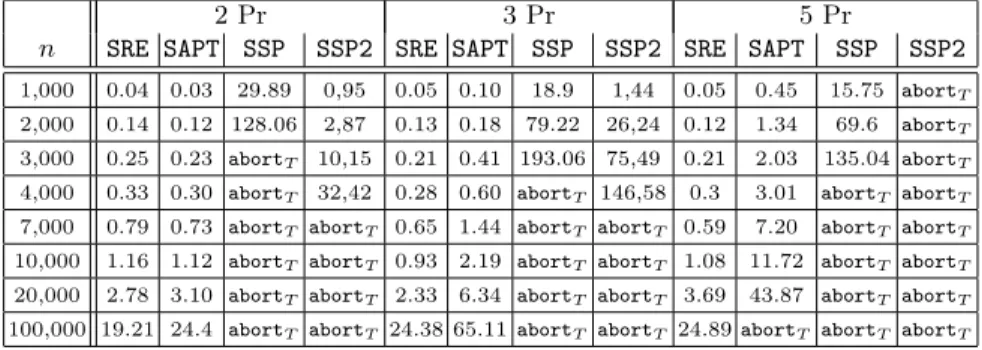
|P| −1, if and only if|i−j| ≤d, where dis named as the distance parameter. Table 1 collects the running time of the symbolic algorithms on random games with linear structures having priorities 2, 3, and 5, and distanced= 25. The results show thatSAPTperforms better than the others in solving games with n≤10,000 nodes and 2 priorities, whileSREis the best performing in all other
1
The tool is available for download from https://github.com/antoniodistasio/sympgsolver 2
2 Pr 3 Pr 5 Pr
n SRE SAPT SSP SSP2 SRE SAPT SSP SSP2 SRE SAPT SSP SSP2
1,000 0.04 0.03 29.89 0,95 0.05 0.10 18.9 1,44 0.05 0.45 15.75 abortT 2,000 0.14 0.12 128.06 2,87 0.13 0.18 79.22 26,24 0.12 1.34 69.6 abortT 3,000 0.25 0.23 abortT 10,15 0.21 0.41 193.06 75,49 0.21 2.03 135.04 abortT 4,000 0.33 0.30 abortT 32,42 0.28 0.60 abortT 146,58 0.3 3.01 abortT abortT 7,000 0.79 0.73 abortT abortT 0.65 1.44 abortT abortT 0.59 7.20 abortT abortT 10,000 1.16 1.12 abortT abortT 0.93 2.19 abortT abortT 1.08 11.72 abortT abortT 20,000 2.78 3.10 abortT abortT 2.33 6.34 abortT abortT 3.69 43.87 abortT abortT 100,000 19.21 24.4 abortT abortT 24.38 65.11abortT abortT 24.89abortT abortT abortT
Table 1.Runtime executions of the symbolic algorithms
cases. Also, they show that SSPandSSP2 have the worst performances in all instances, withSSPovercomingSSP2 of more than 200 seconds on games with 3,000 nodes. In Table 2 we collect the execution time of the explicit algorithms on the same set of games. The results highlight that the explicit algorithms are faster than the symbolic ones in all instances.
2 Pr 3 Pr 5 Pr
n RE APT SPM RE APT SPM RE APT SPM
1,000 0.0008 0.0006 0.0043 0.0008 0.0007 0.0049 0.0008 0.0008 0.0053 2,000 0.0015 0.0012 0.0084 0.0017 0.0016 0.0096 0.0019 0.0029 0.011 3,000 0.0023 0.0017 0.012 0.0025 0.0022 0.014 0.0029 0.0073 0.020 4,000 0.0031 0.0022 0.016 0.0033 0.0028 0.019 0.0035 0.0066 0.027 7,000 0.0051 0.0039 0.025 0.0053 0.0048 0.032 0.0056 0.012 0.039 10,000 0.0065 0.0057 0.035 0.0067 0.0076 0.046 0.0069 0.018 0.051 20,000 0.013 0.011 0.078 0.014 0.021 8.32 0.17 0.019 107.2 100,000 0.094 0.081 0.44 0.099 0.10 1.47 0.10 0.59 80.37
Table 2.Runtime executions of the explicit algorithms
Ladder Games. In a ladder game, every node in Pi has priorityi. In addition, each node v∈P has two successors: one in P0 and one in P1, which form a node
pair. Every pair is connected to the next pair forming a ladder of pairs. Finally, the last pair is connected to the top. The parameterm specifies the number of node pairs. Formally, a ladder game of index m is G = (P0,P1,Mv,p) where
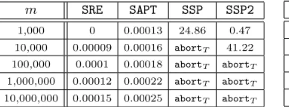
P0={0,2, . . . ,2m−2}, P1={1,3, . . . ,2m−1}, Mv ={(v, w)|w≡2mv+ifor i∈ {1,2}}, andp(v) =v mod2. Tables 3 and 4 report the benchmarks.
The benchmarks indicate thatSREandSAPToutperform their explicit versions, showing an excellent runtime execution even on fairly large instances. Indeed, while RE needs 6.31 seconds for games with index m = 10M, SRE takes just 0.00015 seconds. Benchmarks also show thatSSPandSSP2 have yet the worst performance.
Clique Games. Clique games are fully connected games without self-loops, where P0 (resp., P1) contains the nodes with an even index (resp., odd) and
m SRE SAPT SSP SSP2 1,000 0 0.00013 24.86 0.47 10,000 0.00009 0.00016 abortT 41.22 100,000 0.0001 0.00018 abortT abortT 1,000,000 0.00012 0.00022 abortT abortT 10,000,000 0.00015 0.00025 abortT abortT
Table 3.Runtime executions of the sym-bolic algorithms on ladder games.
m RE APT SPM 1,000 0.0007 0.0006 0.002 10,000 0.006 0.005 0.0017 100,000 0.057 0.054 0.18 1,000,000 0.59 0.56 1.84 10,000,000 6.31 5.02 20.83
Table 4.Runtime executions of the ex-plicit algorithms on ladder games. clique games is the high number of cycles, which may pose difficulties for certain algorithms. Formally, a clique game of index n is G = (P0,P1,Mv,p) where
P0={0,2, . . . , n−2}, P1={1,3, . . . , n−1},Mv ={(v, w)|v6=w}, andp(v) =v.
Benchmarks on clique games are reported in Tables 5 and 6. n SRE SAPT SSP SSP2
2,000 0.007 0.003 5.53 abortT 4,000 0.018 0.008 19.27 abortT 6,000 0.025 0.012 39.72 abortT 8,000 0.037 0.017 76.23 abortT
Table 5.Runtime executions of the sym-bolic algorithms on clique games
n RE APT SPM
2,000 0.021 0.0105 0.0104 4,000 0.082 0.055 0.055 6,000 0.19 0.21 0.22 8,000 0.35 0.59 0.63
Table 6.Runtime executions of the ex-plicit algorithms on clique games
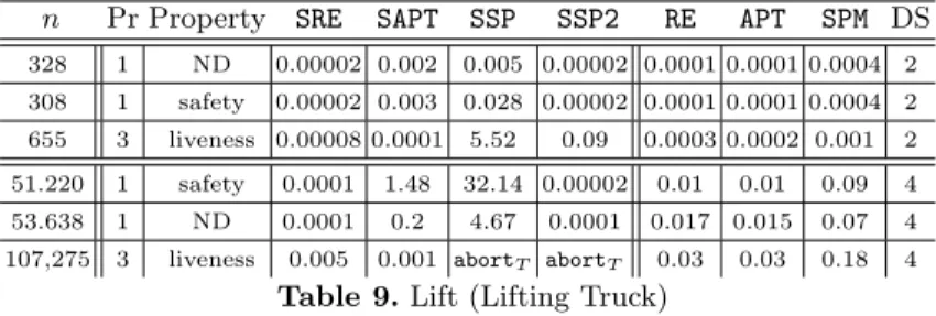
Benchmarks show thatSAPTis the best one among the symbolic algorithms in all instances,SAPTandSREoutperform the explicit ones (as in ladder games), and the symbolic versions ofSPMdo not show good results even on small games. Finally, we evaluate the symbolic and explicit approaches on some practical model checking problems as in [16]. Specifically, we use models coming from: the Sliding Window Protocol (SWP) with window size (WS) of 2 and 4 (WS represents the boundary of the total number of packets to be acknowledged by the receiver), the Onebit Protocol (OP), and the Lifting Truck (Lift). The properties we check on these models concern: absence of deadlock (ND), a message of a certain type (d1) is received infinitely often (IORD1), if there are infinitely many read steps then there are infinitely many write steps (IORW), liveness, and safety. Note that, in all benchmarks, data size (DS) denotes the number of messages.
n Pr Property SRE SAPT SSP SSP2 RE APT SPM WS DS
14,065 3 ND 0.00009 0.00006 3.30 0.0001 0.004 0.004 0.029 2 2 17,810 3 IORD1 0.0003 0.0005 abortT 85.4 0.006 0.006 0.037 2 2 34,673 3 IORW 0.0006 0.0008 164.73 56.44 0.015 0.014 0.053 2 2 2,589,056 3 ND 0.0002 abortT abortT 0.29 1.02 0.93 9.09 4 2 3,487,731 3 IORD1 abortT abortT abortT abortT 1.81 1.4 17.45 4 2 6,823,296 3 IORW 0.3 abortT abortT abortT 3.87 3.13 22.26 4 2
Table 7.SWP (Sliding Window Protocol)
As we can see, by comparing Tables 7, 8, and 9, the experiments indicate more nuanced relationship between the symbolic and explicit approaches. Indeed,
n Pr Property SRE SAPT SSP SSP2 RE APT SPMDS
81,920 3 ND 0.00002 31.69 1.37 0.0016 0.031 0.034 0.22 2 88,833 3 IORD1 0.0027 0.003 abortT abortT 0.036 0.0038 0.27 2 170,752 3 IORW 14.37 98.4 abortT abortT 0.07 0.07 0.47 2 289,297 3 ND 0.0001 154.89 12.3 0.0058 0.13 0.12 1.34 4 308,737 3 IORD1 0.0088 0.009 abortT abortT 0.14 0.13 1.37 4 607,753 3 IORW 43.7 abortT abortT abortT 0.29 0.27 2.06 4
Table 8.OP (Onebit Protocol)
n Pr Property SRE SAPT SSP SSP2 RE APT SPM DS
328 1 ND 0.00002 0.002 0.005 0.00002 0.0001 0.0001 0.0004 2 308 1 safety 0.00002 0.003 0.028 0.00002 0.0001 0.0001 0.0004 2 655 3 liveness 0.00008 0.0001 5.52 0.09 0.0003 0.0002 0.001 2 51.220 1 safety 0.0001 1.48 32.14 0.00002 0.01 0.01 0.09 4 53.638 1 ND 0.0001 0.2 4.67 0.0001 0.017 0.015 0.07 4 107,275 3 liveness 0.005 0.001 abortT abortT 0.03 0.03 0.18 4
Table 9.Lift (Lifting Truck)
they show a different behavior depending on the protocol and the property we are checking. Overall, we note thatSREoutperforms the other symbolic algorithms in all protocols, although the advantage overREis discontinued. Specifically,SRE is the best performing in checking absence of deadlock in all three protocols, but for IORD1 in the SWP protocol withW S= 2, or for IORW in the OP protocol, RE exhibits a significant advantage. Differently, SAPT and SSP2 show better performances on a smaller number of properties. Moreover, the results highlights that SSPexhibits the worst performances in all protocols and properties.
5
Concluding Remarks
In this paper we have compared for the first time the performances of different symbolic and explicit versions of classic algorithms to solve parity games. To this aim we have implemented in a fresh tool, which we have calledSymPGSolver, the symbolic versions of Recursive [24],APT[17, 21], and the small-progress-measures algorithms presented in [5] and [7].
Our analysis started from constrained random games [22]. The results show that on these games the explicit approach is better than the symbolic one, exhibiting a different behavior than the one showed in [22]. To gain a fuller understanding of the performances of the symbolic and the explicit algorithms, we have further tested the two approaches on structured games. Precisely, we have considered ladder games, clique games, as well as game models coming from practical model-checking problems. We have showed several cases in which the symbolic algorithms have the advantage over the explicit ones.
Our empirical study let us to conclude that on comparing explicit and symbolic algorithms for solving parity games, it would be useful to have real scenarios and not only random games, as the common practice has been.
References
1. R. Iris Bahar, E. A. Frohm, C. M. Gaona, G. D. Hachtel, E. Macii, A. Pardo, and F. Somenzi. Algebraic decision diagrams and their applications. Formal Methods
in System Design, pages 171–206, 1997.
2. M. Bakera, S. Edelkamp, P. Kissmann, and C. D. Renner. Solvingµ-calculus parity games by symbolic planning. InMoChArt 2008, pages 15–33, 2008.
3. R. E. Bryant. Graph-based algorithms for boolean function manipulation. IEEE
Trans. Comput., pages 677–691, 1986.
4. J. R. Burch, E. M. Clarke, K. L. McMillan, D. L. Dill, and L. J. Hwang. Symbolic model checking: 10ˆ20 states and beyond. InLICS 1990, pages 428–439, 1990. 5. D. Bustan, O. Kupferman, and M. Y. Vardi. A measured collapse of the modal
µ-calculus alternation hierarchy. InSTACS 2004, pages 522–533, 2004.
6. C. S. Calude, S. Jain, B. Khoussainov, W. Li, and F. Stephan. Deciding parity games in quasipolynomial time. InSTOC 2017, pages 252–263, 2017.
7. K. Chatterjee, W. Dvor´ak, M. Henzinger, and V. Loitzenbauer. Improved set-based symbolic algorithms for parity games. InCSL 2017, pages 18:1–18:21, 2017. 8. E.M. Clarke and E.A. Emerson. Design and Synthesis of Synchronization Skeletons
Using Branching-Time Temporal Logic. InLP 1981, LNCS 131, pages 52–71, 1981. 9. E.M. Clarke, O. Grumberg, and D.A. Peled. Model Checking. MIT Press, 2002. 10. C. Eisner and D. A. Peled. Comparing symbolic and explicit model checking of a
software system. InSPIN 2002, pages 230–239, 2002.
11. E.A. Emerson and C. Jutla. Tree Automata, µ-Calculus and Determinacy. In
FOCS 1991, pages 368–377, 1991.
12. M. Jurdzinski. Deciding the Winner in Parity Games is in UP∩co-Up.Inf. Process.
Lett., 68(3):119–124, 1998.
13. M. Jurdzinski. Small Progress Measures for Solving Parity Games. InSTACS 2000, LNCS 1770, pages 290–301, 2000.
14. M. Jurdzinski and R. Lazic. Succinct progress measures for solving parity games.
InLICS 2017, pages 1–9, 2017.
15. G. Kant and J. van de Pol. Generating and solving symbolic parity games. In
GRAPHITE 2014, pages 2–14, 2014.
16. J.J. A. Keiren. Benchmarks for parity games. InFSEN 2015, pages 127–142, 2015. 17. O. Kupferman and M. Y. Vardi. Weak Alternating Automata and Tree Automata
Emptiness. InSTOC 1998, pages 224–233, 1998.
18. O. Kupferman, M.Y. Vardi, and P. Wolper. An Automata Theoretic Approach to Branching-Time Model Checking. Journal of the ACM, 47(2):312–360, 2000. 19. K. L. McMillan. Symbolic Model Checking. Kluwer Academic Publishers, 1993. 20. J.P. Queille and J. Sifakis. Specification and Verification of Concurrent Programs
in Cesar. InSP 1982, LNCS 137, pages 337–351, 1982.
21. A. Di Stasio, A. Murano, G. Perelli, and M. Y. Vardi. Solving parity games using an automata-based algorithm. InCIAA 2016, pages 64–76, 2016.
22. D. Tabakov. Evaluation of explicit and symbolic automata-theoretic algorithm. Master’s thesis, Rice University, 2005.
23. T. van Dijk. Oink: an implementation and evaluation of modern parity game solvers.
CoRR, 2018.
24. W. Zielonka. Infinite Games on Finitely Coloured Graphs with Applications to Automata on Infinite Trees. Theor. Comput. Sci., 200(1-2):135–183, 1998.