Energy Monitoring of Energy Harvesting Wireless Sensor Networks

(1)

Energy Monitoring of Energy Harvesting Wireless

Sensor Networks

By

Sabir Salah Mahmoud Mogalid

17875

Dissertation submitted in partial fulfilment of the requirements for the

Degree of Study (Hons) (Electrical and Electronics)

FYP II Jan and 2016

Universiti Teknologi PETRONAS

Bandar Seri Iskandar

31750 Tronoh

(2)

I

CERTIFICATION OF APPROVAL

Energy Monitoring of Energy Harvesting Wireless Sensor Networks by

Sabir Salah Mahmoud Mogalid 17875

A project dissertation submitted to the Electrical and Electronics program Universiti Teknologi PETRONAS in partial fulfilment of the requirement for the

BACHELOR OF ENGINEERING (Hons) (ELECTRICAL and ELECTRONICS)

Approved by, _____________________

(Dr. Micheal Drieberg)

UNIVERSITI TEKNOLOGI PETRONAS TRONOH, PERAK

(3)

II

CERTIFICATION OF ORIGINALITY

This is to certify that I am responsible for the work submitted in this project, that the original work is my own except as specified in the references and acknowledgements, and that the original work contained herein have not been undertaken or done by unspecified sources or persons.

__________________________________ SABIR SALAH MAHMOUD MOGALID

(4)

III

ABSTRACT

Understanding the power characteristics of Wireless Sensor Networks is important, as it will help better understand the system and therefore suggesting ways of improving it. A way to monitor the energy consumption of WSNs is needed. The energy consumed by these WSNs tends to be very small and difficult to measure and that is because the consumed current can be relatively small, in microamperes’ range. Besides the relatively small energy, data loggers that used to monitor the energy are costly and it will be very costly to monitor the energy of multiple nodes. In this paper, an energy monitor that is able to measure small energy has been developed to monitor the energy of energy harvesting WSN. The energy harvesting WSN consists of three main components: the mote, the battery and the energy-harvesting module. The circuitry of each one of these three main components has been built to measure their current and voltage. A low cost data logger to sample the voltage and current data has been built that will be able to sample and store the energy profile of all of the three main components. Data have been visualized through a MATLAB graphical user interface.

(5)

IV

ACKNOWLEDGEMENT

This work would not be possible without the blessings of Allah.

This work would not be possible without the enlightened supervision of the esteemed Dr. Micheal Drieberg, by providing his kind assistance and endless support, and by giving his precious feedback.

This work would not be possible without the help of Mr. Muhammad Alif Afiq for helping with the printed circuit board.

This work would not be possible without the coordination of UTP.

(6)

V

LIST OF FIGURES:

Figure 1: Typical WSN deployment [1]. ... 1

Figure 2: Typical Architecture of an energy monitor [3] ... 4

Figure 3: Low side current sensing [4] ... 6

Figure 4: High-side current sensing [4] ... 6

Figure 5: A block diagram of an energy harvesting WSN and the test points ... 12

Figure 6 system solar panel ... 13

Figure 7: Rechargeable battery ... 13

Figure 8: MICAz sensor mote ... 13

Figure 9: INA 210 op-amp [6] ... 15

Figure 10: Swing to V+ and to GND [6] ... 17

Figure 11: Unidirectional Application Schematic [6] ... 17

Figure 12: Bidirectional Application Schematic [6] ... 18

Figure 13: Arduino Mega and Ethernet shield with SD card slot ... 18

Figure 14: the accuracy of the ADC VS the ADC clock frequency ... 19

Figure 15: switch schematic ... 21

Figure 16 : Make-before-break & Break-before-make switches ... 21

Figure 17: Sample of the program ... 23

Figure 18: WSN consisting of two nodes ... 25

Figure 19: energy monitoring schematic ... 26

Figure 20: current profile of MICAz with 2 seconds transmission intervals ... 27

Figure 21: voltage profile of MICAz with 2 seconds transmission intervals ... 27

Figure 22:: current profile of MICAz When the transmission rate is 4 seconds ... 28

Figure 23: voltage profile of MICAz when the transmission rate is 4 seconds ... 28

Figure 24: Mote current profile using the ... 29

Figure 25: current profile of MICAz when the sensor mote is off ... 30

Figure 26: voltage profile of MICAz when the sensor mote is off ... 31

Figure 27: current profile of the solar panel ... 32

Figure 28: Voltage profile of the solar panel ... 32

Figure 29: Analog switch top view ... 33

(9)

VIII

LIST OF TABLES:

Table 1: Advantages and disadvantages of low-side and high-side current sensing ... 7 Table 2: Comparison between the proposed design features and other already-existing energy monitors features ... 14 Table 3: the sampling frequency VS the number of channels ... 19 Table 4: analog switch Function table ... 33

(10)

IX

ABBREVIATIONS AND NOMENCLATURES:

WSN Wireless Sensor Network

ADC Analog to Digital Convertor

SPOT Scalable Power Observation Tool

Op-amp Operational Amplifier

N.C. Normal Closed contact

N.O. Normal Open contact

(11)

1

CHAPTER 1 INTRODUCTION

1.1 Background:

Wireless Sensor Networks (WSNs) are a set of sensor nodes distributed in different locations to monitor and sense the physical and environmental factors such as temperature, pressure and sound, etc. as shown in Figure 1.

Figure 1: Typical WSN deployment [1].

The importance of WSNs is huge and their applications are numerous.Deploying a WSN with temperature and humidity sensors can be used to monitor the weather. The sensor nodes can be placed on different locations. The readings and the collected data can be sent to a central computer for further analysis.Machine monitoring is another application of WSN. The induction motor can be taken as an example of a monitored industrial device where the motor current and vibration signals are monitored for further analysis and post-processing.

WSN consist of multiple detection stations called sensor nodes. Every sensor node consists of a transducer (sensor), a microcomputer and a transceiver. The power of each

(12)

2

sensor node is derived from a non-renewable battery or from an energy harvesting source [2]. The non-renewable batteries need to be replaced from time to time when they get consumed. Replacing non-renewable batteries may be frustrating, cost and time consuming especially when the number of sensor nodes is huge or if they are placed at a far distance, therefore, traditional power sources may not be the best option to use in WSNs. On the other hand, energy harvesting technology has improved rapidly over the past several years. Energy can be harvested from different sources such as light, vibration, flow and motion. The harvested energy can be stored and used to self-power the WSN. This type of WSNs which have the feature of harvesting energy is called energy harvesting wireless sensor networks.

The nodes of WSNs are usually mounted autonomously and they are left for long times. Analyzing and investigating the energy profile of these WSNs will help improving their power-efficiency. The characteristics of the energy profile will help providing an insight and recommendations on how to improve the power consumption of WSNs, that is, before proposing means of improving the power consumption, we need to understand the characteristics and properties of the power consumed from WSNs.

The energy has mainly been assessed by various simulation software. However, the simulation results are not as accurate as the data measured using an actual energy monitor. As a result, a variety of actual energy monitors are available nowadays.

The main focus on this project would be on the energy monitoring part. On this project, an energy monitor for energy harvesting WSNs is to be developed which will help analyze and investigate the power consumption of these WSNs

1.2 Problem statement:

The available energy monitors are very expensive, typically, one unit of an energy monitor costs RM 10,000. The one unit can be used to monitor the performance of only one sensor node, while a typical WSN consists of multiple sensor nodes. Imagine a scenario where a WSNs consists of 10 sensor nodes, this will result in very costly energy monitors to record the energy for 10 sensor nodes with a total cost of RM 100,000.

(13)

3

On the other hand, energy monitors themselves consume energy. It’s unconventional for the energy monitors to consume a big portion of energy which will result on an added cost to the energy monitor.

The project will address the problem of the high power and high cost energy monitors which are used to evaluate and monitor the energy of energy harvesting WSNs.

1.3 Objectives:

The objectives of the project are:

- To develop a low power, reliable and cost effective energy monitor for energy harvesting WSNs.

- To develop a decent graphical user interface for the ease of use and visualization of the collected data.

(14)

4

CHAPTER 2 LITERATURE REVIEW

Testing the power efficiency of a WSN can be frustrating, deploying and installing the equipment to perform power measurements is tedious. Various simulation software are available to predict the energy in WSNs. The simulation software counts the time taken in sending, receiving, and computing, and multiplying that by figures taken from data sheets or isolated (single-node) power measurements. However, as mentioned earlier, the simulation results are not as accurate as the results measured using an actual energy monitor. As a result, a variety of actual energy monitors are available nowadays.

2.1 Typical Architecture of an energy monitor

The typical architecture of actual energy metering circuits consists of a shunt resistor that will be connected to the mote to measure the current. The voltage across the shunt resistor is proportional to the current. The voltage across the shunt resistors and the node’s voltage are connected to amplifiers (if needed) before they get attached to the ADC, the ADC will convert the analog signal into a digital one. The digital signal will be filtered first before multiplying the voltage and current samples, and finally the results will be stored before they get transferred for further analysis and investigation.

(15)

5

2.2 Designing an energy monitor factors:

There are different factors that we need to consider in the designing process. These factors include the dynamic range, the sampling rate, the type of current sensing, the current direction, the current range, perturbation, ease of integration and usability and other factors related to shunt resistor [3], [4].

2.2.1 Dynamic range:

The dynamic range is the rate of largest measurable amount to the smallest measurable amount. In this case, the dynamic range is the rate between the highest current that will be measured during the active mode of the sensor node to the lowest current that will be measured during sleep mode. Normally the design requires a high dynamic range which is in turn translated into an ADC with a high resolution. 10 bits ADC provides 1000:1 dynamic range while 14 bits ADC can provide up to 10,000:1 dynamic range. However, the greater the number of ADC bits, the more expensive it will be.

2.2.2 Sampling rate:

The sampling rate is the number of samples/ second. In this exact case, the sampling rate depends on how fast the current or the voltage signal change, for example if the current signal may change every 0.5 milliseconds, a sampling frequency of 2 KHz is needed to capture these changes. The rate of change of the signal can be obtained from the datasheets of the device under test.

2.2.3 Type of current sensing:

As mentioned earlier, to measure the current, a shunt resistor will be used. The voltage across the shunt resistor is proportional to the current. An op-amp will be used to amplify the voltage, as the voltage from the shunt resistor is relatively small. The shunt resistor can be used in two ways: low-side current sensing and high-side current sensing. Each of these methods has its advantages and disadvantages.

2.2.3.1 Low-side current sensing:

Low side current sensing occurs when the shunt resistor is placed between load or the device under test and the ground as shown in figure 3:

(16)

6

Figure 3: Low side current sensing [4]

The sensed voltage across the shunt resistor will be fed into an op-amp, therefore, this sensed voltage should be in the range of the input common mode voltage of the op-amp, which for low-side current sensing is close to zero.

Since the common mode voltage of the sensed signal is close to zero, a low voltage and inexpensive amplifier can be used. However, the problem with the low-side current sensing is that, it changes the actual ground of the system, system GND = ILOAD * RSHUNT. Many applications cannot tolerate the ground disturbance and therefore this method can’t be used. Another problem with low-side current sensing is that, short-circuit that happens accidently between the load and the ground will go undetected.

2.2.3.2 High-side current sensing:

High-side current sensing occurs when the shunt resistor is placed between the power supply and the load as shown in figure 4:

Figure 4: High-side current sensing [4]

The advantages of the high-side current sensing are that; they allow detecting accidental short-circuit errors. Another major advantage is that; it also eliminates ground

(17)

7

disturbance. However, for high-side current sensing, the common mode voltage of the shunt resistor is close to the supply voltage, therefore the op-amp input common mode range should include the supply voltage.

The following table will summarize the advantages and disadvantages of the two approaches:

High-Side Low-Side

Strength - Can detect load shorts to ground - Eliminates ground disturbance

- Vcm = 0V

- Inexpensive

challenges Vcm = Vsupply - Can’t detect load

shorts to ground - Ground

disturbance, system GND = ILOAD

* Rshunt

Table 1: Advantages and disadvantages of low-side and high-side current sensing

2.2.4 Current direction:

For current sensing, the current can be uni-directional or bi-directional. Some amplifiers allow only uni-directional current measurements while others allow bi-directional current measurements.

2.2.5 Current range implications:

The current range will determine two key specifications:

1- System gain: the product of the amplifier Gain * IMAX is supposed to be less than the maximum voltage of the next component in the chain, which is the controller in this case.

2- Minimum differential voltage from the sensing resistor: the minimum voltage developed across the shunt resistor should be large enough compared to the offset voltage of the op-amp.

(18)

8 2.2.6 Shunt resistor factors:

There are two factors need to be considered when choosing a shunt resistor or a current sensing resistor:

- Minimum current accuracy

- Maximum current power dissipation (size and cost)

It’s a tradeoff between accuracy and the maximum power dissipation during maximum current of the solar panel. The larger the value of the resistor, the greater the voltage developed across it, therefore higher accuracy, that is larger voltages are easier to measure. However, a higher value resistor will result in a higher power dissipation.

The shunt resistor has a maximum value which is determined by the following equation:

Maximum Resistor Value =𝑉𝑜𝑢𝑡/𝑔𝑎𝑖𝑛 (𝑜𝑓 𝑜𝑝−𝑎𝑚𝑝)

𝑚𝑎𝑥𝑖𝑚𝑢𝑚 𝑙𝑜𝑎𝑑 𝑐𝑢𝑟𝑟𝑒𝑛𝑡

The power dissipation caused by the shunt resistor can be calculated as follows:

Power dissipation = R (shunt) * I2_(load)

2.2.7 Perturbation:

The energy meter is supposed not to affect the normal operation of the sensor node. Means of decoupling the node under test and the energy meter are needed.

2.2.8 Ease of integration and usability:

Ease of integration and usability requires the system to be easy to install and easy to use with the WSN.

2. 3 Existing Energy Monitors

Many energy monitors have been developed for the sake of monitoring the energy in WSN. SPOT and PowerBench are examples of energy monitors. The main idea behind the power measurements is by monitoring the current and the voltage of the mote. 2.3.1 SPOT

SPOT is a meter developed to perform micro-power measurements. SPOT is an abbreviation for a Scalable Power Observation Tool. The tool is mainly dedicated for high dynamic range power measurements. The difference in power consumption between the

(19)

9

active state and sleep state is large in terms of order of magnitude which requires a high dynamic range to be able to obtain the power consumption with an accurate resolution. SPOT provides a dynamic range of 10000:1 which is sufficient to obtain the small changes of power consumed by motes. Besides, SPOT provides a high sampling rate up to 5-10 KHz for the power measurements. During the active mode, there are short-duration power spikes that require a high sampling rate. SPOT is efficiently able to capture these short duration power spikes. As other commercially devices available, SPOT uses a shunt resistor connected to the mote for power measurements, the voltage across this resistor is directly proportional to the current through the resistor which is in turn proportional to the power. In Spot, the voltage is assumed to be constant. The voltage and current are multiplied digitally to obtain the power.

To obtain the high dynamic range, a Voltage to Frequency Converter(VFC) has been used in SPOT. Obtaining 10000:1 dynamic range needs at least a 14 bits ADC if a one is to be used. But as mentioned, VFC has been used. The output of the VFC is connected to two counters. The first counter is used to count the power pulses from the VFC which is proportional to the voltage which is in turn proportional to the power. The other counter is used to measure the time, by measuring the number of pulses during a predetermined time, the current with 45,000:1 dynamic range can be obtained. [3]

2.3.2 PowerBench:

PowerBench does not differ much from SPOT. PowerBench uses a shunt resistor to measure the current with a resolution of 30uA. PowerBench uses a 12 bits ADC and a cut-off frequency of 5 KHz which is in turn translated to 10 KHz sampling frequency. The range of current covered by PowerBench is (0-65) mA. In PowerBench, some considerations have been taken into account to avoid some of SPOT disadvantages as they consider it a high-cost energy meter that is not suitable for large scale deployment. Another disadvantage of SPOT is that, the used oscillator and the VFC can be sources of significant noise in the system. To avoid the mentioned disadvantages, PowerBench mainly suggested to use a single-chip successive approximation ADC solution [5].

(20)

10 The following table is to summarize the differences:

Author Title Year Method Demerit

Xiaofan Jiang, Prabal Dutta.

Micro Power Meter for Energy Monitoring of Wireless Sensor Networks at Scale 2003 Actual hardware, using a VFC to monitor current

- Costly for large scale deployment - VFC clock is a source of noise Ivaylo Haratcherev, Gertjan Halkes, et al. PowerBench: A Scalable Testbed Infrastructure for Benchmarking Power Consumption 2008 Actual hardware using a 12 bits ADC to monitor current

(21)

11

CHAPTER 3 METHODOLOGY

As mentioned earlier, an energy monitor for energy harvesting WSNs is to be developed. This section will be focusing on the research methodology and a general overview of the steps that will be taken in order to achieve the objectives. First of all, an extensive literature review must be carried out. The literature review is followed by identifying the specs of the main blocks that will be tested (energy harvester, mote and battery). Next, the main system components is to be used. After the components have been selected, the energy monitor that is to be built. In addition to defining the main building blocks as the micro-controller and the communication protocol that will be used to transfer the data to PC.

Choosing the components

Testing the components to obtain the energy measurements

Developing a graphical user interface for data visualization Defining the system under test

specifications Literature review

(22)

12

3.1 Literature review:

An extensive literate review must be carried out in order to define, identify and analyze the existing techniques of implementing an energy monitor. Comparison between these different techniques is needed in order to determine the best and the most cost effective way of implementing a high dynamic range and high sampling frequency energy monitor.

3.2 Defining the system under test specifications

3.2.1 Test points block diagram:

As mentioned earlier, the system under test is an energy harvesting WSN. The system consists of a solar panel as an energy harvester, and a storage battery to store the energy and finally the mote itself. There are different voltage regulators to regulate the power voltage between these main units. The energy monitor that is to be developed will mainly monitor the energy for three different test points. The first test point is the output energy from the energy harvester, the second test point is at the battery, and finally the third test point is at the mote itself as shown in Figure 5.

(23)

13 3.2.2 Test points specifications:

- Solar Panel: SOLAREX MSX-005 BP SOLAR panel 0.5W 3.3V 150mA

Power Rating 500mW

Power Voltage Max 3.3V Current at P Max 150 mA Open Circuit Voltage 4.6V Short Circuit Current 160mA

- Battery: Nimh rechargeable battery (1.2v) 1500mAh

Nominal voltage 1.2V Rated capacity (mAh) 1500 mAh

- Mote: MICAz

Maximum Current 30 mA Minimum Current 35 uA

Battery 2X AA batteries External Power 2.7 V - 3.3 V

3.3 The system specifications and choosing the components

The architecture of the energy monitor to be built is quite similar to other exiting energy monitors, the main difference will be in the way the current measurements are taken and the main components under test (energy harvester, mote and battery).

3.3.1 The dynamic range of the system

Some of the existing energy monitors use a 14 bits ADC that will provide a 10000:1 dynamic range. However, that will increase the cost of energy monitor, other energy

Figure 6 : system solar panel

Figure 7: Rechargeable battery

(24)

14

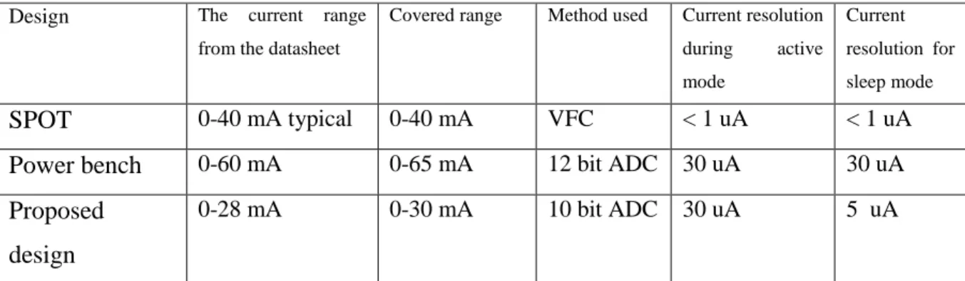
monitor is using a VFC attached to a counter and as mentioned before this will result in a high cost energy monitor, in this project a 10 bits ADC is to be used, two ADC channels will be dedicated for the current measurements for the mote. The first one is to take the current measurements when the node is in active mode, the other channel will take the measurements when the node is in sleep mode. This way, for the active mode, a dynamic range of 1000:1 to explore the active mode current. From the datasheet it’s stated that the active mode current can reach up to 28 mA. The device will be designed in such a way that it will take the measurements in the range of (0-30 mA) distributed over 1000 ADC steps which will result in 30 uA resolution for the active mode. On the other hand, for sleep mode, the current can reach up to 35 uA. The conditioning circuitry is to be designed to cover the range from 0 to 5mA distributed over 1000 ADC steps which will produce 5u current resolution.

Using two channels to measure the current will provide more descriptive current profile for sleep mode and active mode separately.

Design The current range from the datasheet

Covered range Method used Current resolution during active mode Current resolution for sleep mode SPOT 0-40 mA typical 0-40 mA VFC < 1 uA < 1 uA

Power bench 0-60 mA 0-65 mA 12 bit ADC 30 uA 30 uA

Proposed design

0-28 mA 0-30 mA 10 bit ADC 30 uA 5 uA

Table 2: Comparison between the proposed design features and other already-existing energy monitors features 3.3.2 The type of current sensing:

In the case of the energy monitor, ground disturbance may affect the performance of the mote and the rest of the system components. The measurement of the current from the system is very sensitive as well, and therefore, a high side current sensing has been selected.

After we have chosen the type of sensing, there are some other considerations need to be taken into account for the current measurement.

(25)

15 3.3.3 The current direction:

In the case of this specific energy monitor, the current from the solar panel is uni-directional to feed the rest of the system components. The mote current is the same as the solar panel in term of direction; the current will only flow in to the mote allowing it to operate. However, for the battery, the current is bi-directional since the current will go in to charge up the battery and will go out of the battery to feed the mote when needed.

Some amplifiers allow only uni-directional current measurement while others allow bi-directional current measurement.

3.3.4 Shunt resistor calculations:

Before performing shunt resistor calculations, a specific amplifier should be chosen as the gain of the op-amp will be used in calculating the value of the shunt resistor.

Amplifier (INA210) has been chosen as it comes with the following specifications:

- Common mode voltage = -0.3 to 26 V: as we can see the maximum value of the input common mode voltage is 26V which is

relatively high to include the 5V power supply or 3.3V power supply.

- Bidirectional: it can sense bi-directional current as in the case of the battery

- Offset error = 35uV, the offset error is very small and it’s in term of a few micro-volts.

- Gain = 200: the gain of the op-amp is fixed, and it has a value of 200. The internal network and connections of the op-amp provides an accurate gain comparing to the other methods of using resistors to determine the gain of the op-amp. When using resistors, these resistors have error regarding their resistance and therefore that will affect the accuracy of the measurements.

- Price = 0.76 US$: as we can see that the price is low.

From the equation and by using INA210 and an Arduino controller runs at 5V:

Maximum Resistor Value =𝑉𝑜𝑢𝑡/𝑔𝑎𝑖𝑛 (𝑜𝑓 𝑜𝑝−𝑎𝑚𝑝)_{𝑚𝑎𝑥𝑖𝑚𝑢𝑚 𝑙𝑜𝑎𝑑 𝑐𝑢𝑟𝑟𝑒𝑛𝑡}

(26)

16

Component Gain Maximum current

Calculated RMAX value

Available values

solar panel 200 160 mA 0.15 ohm 0.15 ohm

battery 200 160 + 40 mA 0.120 ohm 0.10 ohm Mote (high range) 200 30 mA 0.8 ohm 0.75 ohm Mote (low range) 200 5 mA 4.8 ohm 4.7 ohm

Note: The Vout is the maximum output of the op-amp, a detailed description will be discussed in the op-amp session below.

Note: the charging battery current is assumed to be 160 mA as this is the maximum current that the solar panel can provide, in addition to the 160 mA charging current, the discharging current must be added to calculate the battery maximum current, therefore, a 30 mA will be added to the 160mA. 40 mA has been considered instead of 30 mA to make calculations easier and to help find standard resistors for the bi-directional current measurement. A more detailed information about bi-directional measurement will be discussed in the op-amp section bellow.

3.3.5 Op-amp considerations:

The concept of using an op-amp might seem easy, but to actually use one in the real world that requires a proper understanding of the different characteristics of the op-amp.

3.3.5.1 Powering-up the op-amp implications:

When using an op-amp, the output of the op-amp is bounded by the supply voltages of the op-amp (the rails of the op-amp), the output of the op-amp doesn’t reach the rails of the supply, for example, if 0V and a 5V are used as the supply voltage, the output of the op-amp won’t reach 5V but rather it will swing to a value that is close to the 5V, 4.8V in the case of this specific op-amp (5V-0.2V). The output also won’t swing to reach 0V but rather 0.05V (0+0.05) as explained in figure 10.

Note: the maximum values (V+) – 0.2V and VGND +0.05V have been chosen as they are the worst cases.

The values of the shunt resistors must to be calculated in a way that the maximum current will produce a voltage that is equal or less than the maximum output voltage.

(27)

17

Figure 10: Swing to V+ and to GND [6]

3.3.5.2 Bidirectional op-amp measurements:

Before talking about the bi-directional mechanism, lets first start by the uni-directional schematic.

By refering to figure 11, the differential input is connected to IN- and IN+, the supply voltage is then connected to V+ to power-up the op-amp and its also is connected to the ground through a 0.1 uF bypass capacitor to stablize the supply voltage. The system ground is then connected to GND.

The REF pin is a reference for the output that corresponds to a zero-input conditions (the differential input voltage across IN- and IN+ is zero V).

Figure 11: Unidirectional Application Schematic [6]

In the case of bidirectional application (figure 12), the connections are the same except for REF pin. As mentioned before, the REF correspends to the output when the

differential input is zero, for example if REF is 2.5V, and if the differential input voltage across IN- and IN+ is 0V, then the output will be 2.5V. In bi-directional applications, for positive differential signals, the output will increase above the REF, and if it’s a negative differential signals which indicates a current at the opposite direction, the output will decrease bellow the REF.

(28)

18

Figure 12: Bidirectional Application Schematic [6] 3.3.6 Arduino as a data logging device:

As mentioned earlier, the Arduino will be used as a data logging device to sample the current and the voltage data. Arduino Mega has been chosen as it has a sufficient number of analog channels (7 channels are needed and Mega has 16 channels).

To use the Arduino as a data logging device, a shield with an SD card slot is needed. Data logging shield and Ethernet shield have SD card slots, Ethernet shield has been chosen because of its availability and its low price comparing to Data logging shield.

Figure 13: Arduino Mega and Ethernet shield with SD card slot

The sampling rate depends on the number of channels and the ADC clock, i.e., the frequency at which the ADC will operate. Table 3 shows the sampling frequency based on the number of channels:

(29)

19

Table 3: the sampling frequency VS the number of channels

When increasing the ADC clock, the number of effective ADC bits will reduce,i.e., the accuracy will decrease. Figure 14 describes the relationship between the effective number of bits and the ADC clock frequency.

(30)

20

Note, the ADC frequency is the freequency in which the ADC operates. When the frequency increases, the effective number of ADC bits decreases and this will affect the sampling accuracy and the resolution. So it’s a trade off between the speed and the accuracy, a wise decision should be taken.

In this specific case for the energy monitor, we are going to use 7 channels as follows: 3 voltage channels for the solar panel, the mote and the battery,one channel for each, other 4 channels are to be used to measure the current, one for each of the battery and the solar panel and two for the mote as the mote active mode and the mote sleep mote will be monitored in different channels as mentioned earlier.

For this energy monitor, we need to use the maximum possible sampling frequency with a good acceptable effective number of bits, i.e. resolution. By refering to figure 14, for 7 channels, at 1 MHz ADC clock frequency, the

maximum sampling frequency is 6299 Hz but the effective number of bits drops down to 8.6 instead of 10 and hence less accuracy. At 250 KHz and 500 KHz ADC clock frequency, the sampling rate is 2111 Hz and 3791 Hz respectively. 500 KHz ADC clock frequency will be chosen as its effective number of bits (9.4) doesn’t differ much from the 250KHz one which is 9.5, and at the same time the 500KHz ADC clock offers a higher sampling rate.

3.3.7 Switch considerations:

As mentioned earlier, the active mode and the sleep mode will be monitored separately in two different channels, by refereeing to figure 15, we can see that, the positive terminal of the battery is connected to the positive terminal of both the active mode amp (top amp) and the sleep mode amp (bottom op-amp), while the negative terminal of these two op-amps are connected to the load (the mote) through a single-pole, single-throw (SPDT) switch, the switch

(31)

21

will change the path to the mote and therefore to the ground that is connected to the other end of the mote. The current will only go through one of the two paths. One of the most important factors to choose the switch is that, it’s a

make-before-break-switch i.e. before breaking the connection between the mote and the negative terminal of one of the op-amp, it connects between the mote and the negative terminal of the other op-amp. By implementing this mechanism, we will guarantee the continuity of the measurements.

Figure 16 explains two different types of SPDT switches which are: break-before-make and make-before break switch.

Figure 16 : Make-before-break & Break-before-make switches Figure 15: switch schematic

(32)

22

As we see from figure 16, on the first row, during the switching operation, we can see that both of the N.O. (Normal Open contact) and N.C. (Normal Close contact) are both in a break position as it breaks the N.C. connection before it makes the N.O.

connection and that is what’s called break-before-make switching. While on the second row, we can see during the operation that N.C. and N.O. are connected as it makes the N.O. connection before it breaks the N.C. connection. As we can see in the make-before-break switching, at least there is always one point connected, this way will guarantee the continuity of the measurement.

3.4 Graphical user interface

A MATLAB graphical user interface has been developed to display and visualize the data. By referring to figure 17, to configure and connect the Arduino, the COM port to which the Arduino is connected is to be determined in DAQ COM port text box and then connect DAQ button is to be pressed. Now a connection between Arduino and the PC has been stablished through MATLAB.

The sampling frequency and the sampling time are to be entered by user through

Sampling Frequency Hz text box and Sampling time s text box respectively.

Axes 1 is to display the voltage while Axes 2 is to display the current of the selected channel. 1 channel is to be used at a time from the Channel group box. The user can use WSN channel, Battery channel or Solar Panel channel. Now, the data logger is ready to log data and display it. Log data button is to be pressed.

When log data button is pressed, the Arduino will start sampling the data at high sampling rate and store it in the SD card first before sending it to the PC. After the sampling is done for the pre-specified sampling time, the date is sent to the PC. The reason why the samples are stored in the SD card first before sending them to the PC is the speed, sending the samples directly to the PC is done through the serial port which is very slow and the Arduino will not be able to achieve high sampling rate, but when using the SD card, that will allow the Arduino to sample at high speed as the SD card uses SPI protocol which is much faster comparing to the serial port.

(33)

23

The log will be displayed on the log list box. It will show the count of samples, the name of the file to which the data have been saved information about the current process.

After finishing, or to release the serial port to be used by other applications, disconnect DAQ button is to be pressed.

Timeline for FYP I and Key milestones

No. Details/ Week FYP 1

1 2 3 4 5 6 7 8 9 10 11 12 13 14

1 Selection of the project topic 2 Literature review

3 Submission of Extended Proposal

4 Proposal Defense

5 Determining the system requirements

6 Choosing the components for the building blocks 7 Building the signal

condition circuit

8 Submission of Interim Draft Report

9 Submission of Interim Report

(34)

24

Key milestones for FYP 1:

- Selection of the project topic

- Defining the system under test specification

- Choosing the system components and parts

- Ordering the components

- Submission of Interim Draft Report

Timeline for FYP II and Key milestones

No. Details/ Week FYP 2

1 2 3 4 5 6 7 8 9 10 11 12 13 14

1 Testing and troubleshooting the implemented circuit 2 Submission of Progress

Report

3 Developing graphical user interface

4 Testing and deploying the whole system

6 Pre-SEDEX

7 Submission of Draft Final Report

8 Viva

9 Submission of Project Dissertation (Hard Bound)

Key milestones for FYP 2:

- Connecting the components together and building the energy monitoring circuitry

- Setting up the WSN

- Developing the graphical user interface using MATLAB

- Developing the data logger

- Testing all the parts together and obtaining data

(35)

25

CHAPTER 4 RESULTS AND DISCUSSION

This chapter is going to discuss about the experiment settings and the results obtained. The main component of the energy monitor which is the current sensing amplifier, the Arduino as a data logger and the GUI have been tested with the sensor mote while its transmitting date to the getaway. The Arduino has been used as a data logger to capture the data and the MATLAB GUI to visualize and display the data. The switch which will be used to switch between the active and sleep current modes has also been tested and verified

4.1 .1 The op-amp, Arduino and the GUI test

The WSN in figure 18 has been set as micaZ motes (MPR2400CA) have been programmed, one mote to send data [1] and the other one to receive data [3]. the first mote is the base mote which is connected to the PC through MIB520 interface board [4] through USB, the second node is connected to theMica2 Data Acquisition Board

MDA300CA [2] which has temperature and humidity sensors and other ADC channels, let’s call it the sensor mote.

Figure 18: WSN consisting of two nodes

In this experiment, the sensor mote [1] will send temperature and humidity reading to the PC through the base node [4]. The objective of the experiment is to monitor the energy of the sensor mote while its operating and transmitting the sensor data to the PC.

Sensor mote

(36)

26

The energy monitoring circuitry in figure 19 is used to monitor the sensor mote voltage and current, the Arduino will sample the data and store it to the SD card, and when sampling is done, the Arduino sends the data into the PC and displays it in a MATLAB GUI.

Figure 19: energy monitoring schematic

The overall design of the whole system is intended to be used for 7 channels with a maximum sampling frequency of 3791 Hz, however, in this experiment only two channels were used and therefore the maximum frequency can reach up to 11111 Hz when using 500KHz ADC clock(refer to Table 3). In this experiment, the sampling rate was 5000 Hz.

4.1.2 Results and discussion

When using MICAz WSN, the rate of the data transmission can be set, as the sensor mote can transmit data every second or every 4 seconds and so on. Below are the results for 3 different settings, the first one, the sensor mote transmits data every two seconds,

(37)

27

the second one, the sensor mote transmits data every 4 seconds and the last one when the sensor note is off.

When the transmission rate is two seconds:

Figure 20: current profile of MICAz with 2 seconds transmission intervals

(38)

28

When the transmission rate is 4 seconds:

Figure 22:: current profile of MICAz When the transmission rate is 4 seconds

Figure 23: voltage profile of MICAz when the transmission rate is 4 seconds

By referring to figure 20 and 22, we notice that, the current range is from 0-30 mA, which is the expected current range according to the datasheet [6] , which indicates that, the results are valid and the current monitoring op-amp is working as expected.

Another observation is that; for the 2 seconds transmission rate experiment, a consistent pattern appears every 2 seconds, which is indicated by the black oval in figure 20, and under 4 seconds transmission rate experiment, the same pattern appears every 4 seconds (figure 22). This observation confirms that, the obtained data is the current data and it is a valid date.

(39)

29

In figure 21, 23, the voltage is constant during the whole sampling period as expected as it’s the voltage provided by the battery which will appear to be constant during small periods but decrease slightly over time.

We can also see that the signal is noisy and that is because the signal may contain frequency components that are above the range that the sampling frequency is capable of capturing. In this case, any frequency that is above 2.5 KHz (5 KHz/2) the sampling frequency will not be able to capture and may cause the signal to be noisy. By adding an anti-aliasing filter, better results are expected.

Comparing between the developed data logger and industrial data logger DT80:

The current profile has been obtained using off-the-shelf, already proven data logger called DT80. Figure 24 shows the current profile the mote using DT80 with a sampling rate of 200 Hz:

Figure 24: Mote current profile using the

As we can see from figure 24 and by comparing to figure 22, we can see that both of the current profiles are within the range 0-30mA, and both of them stay constant at 24mA.

(40)

30

Also we can see that both of them go up from 24mA to 27/28mA every two seconds and that is due to the setting of the experiment to send data from the transmitter to the

receiver every 2 seconds.

We can notice that, in figure 22, which has been obtained using the newly developed data logger, there are current spikes going up and down, these current spikes don’t appear in the current profile obtained using DT80 (figure 24), and this might be due to the sampling frequency. The sampling frequency of DT80 is 200 Hz (preferable sampling frequency) while for the newly developed data logger is 5000Hz. Since the sampling frequency in the developed data logger is higher than DT80, that means more samples have been obtained within the same period and DT80 didn’t manage to capture these spikes e.g. the time between samples is greater than the time in which the spikes occur.

When the sensor mote is off:

(41)

31

Figure 26: voltage profile of MICAz when the sensor mote is off

When the sensor mote is off, we can see that the current is zero as expected (figure 25). We can see that the voltage did not change as it is the battery voltage and it is a constant value (figure 25) only will change within long time when they are being consumed.

The solar panel Voltage and current:

In addition to the mote, the solar panel has been tested as well; the voltage and the current profile of the solar panel have been obtained. Figure 27 and 28 shows the current and the voltage profiles respectively.

(42)

32

Figure 27: current profile of the solar panel

Figure 28: Voltage profile of the solar panel

As we can see from figure 27, the current is 40 mA. Since, these readings have been taken around 6:00 pm, the value of the current is reasonable since the rated current of the solar panel is 150 mA.

(43)

33

In figure 28, we can see the obtained voltage is 4.4V, and from the datasheet, the open circuit voltage is 4.6V, as we can see, the difference is not major and it might be because of the intensity of the sun light.

4.2.1 The switch test

The analog SPDT switch has been tested and verified, by refering to figure 29, the GND and V+ are connected to the arduino GND and Arduino 5V respectively to power-up the switch.

Figure 29: Analog switch top view

Two different signals are connected to NC (normally closed contact ) and NO (normally open contact), the first signal is a 5V from arduino connected to NO and the second signal is a 3.3V to NC. the output appears at COM pin which is going to be either the NC signal or the NO signal according to table number 4

Table 4: analog switch Function table

For this switch we have two control signals ENbar and IN. in this experiment EN is always connected to Low and IN changes between High and LOW so when IN is Low, NC to COM will be connected and if IN is High, NO to COM will be connected. The IN pin is controlled by the arduino, the output at COM pin is read using the arduino analog channel itself. In the beginning the IN pin is set to High and after that, the COM output is captured, then the IN pin is set to Low and the COM output are obtained. The

(44)

34

Figure 30: Analog switch results:

we can see that, when IN is High, the COM output was 5V which was connected to the NO pin and when IN is Low, the COM output was 3.3V which was connected to NC pin and that is exactly what is expected.

(45)

35

CHAPTER 5 CONCLUSION AND RECOMMENDATIONS

Monitoring the energy and investigating the power profile of WSN is considered as an exciting topic of research in the field of communication that aims to improve the power consumption of WSNs. However, the available energy monitors are very expensive which makes it difficult to monitor the energy of these WSNs. A low power, low cost and reliable energy monitor is to be developed.

The energy monitor under development has the basic building blocks that already exists in the available energy monitors. The advantage of this energy monitor over the existing ones is that, the system will have a complete picture of energy monitoring for energy harvesting WSN as the system will mainly monitor the energy flow for the solar panel, the battery and the mote, while in the existing energy monitors, they only focus on the mote. In addition, the system is using a relatively cheap micro-controller with 10-bit ADC but with implementing switching mechanism to monitor the sleep-mode small current and the active-mode relatively high current in separate channels, which will allow more accuracy and reliability to look into the system.

All of the components have been ordered. Two main tests have been carried out to test the main components, which are the current monitoring amplifier and the switch. The results are satisfying as the current profile is within the range stated in the datasheet with a consistent pattern of data. A decent graphical user interface has been developed using MATLAB and finally the Arduino with Ethernet shield has been tested and verified as a data logging device.

(46)

36

CHAPTER 6 REFERENCES

[1] R. Müller and M. Duller, "SwissQM," ETH Zürich, [Online]. Available: http://www.swissqm.inf.ethz.ch/.

[2] "techtarget," June 2006. [Online]. Available:

http://searchdatacenter.techtarget.com/definition/sensor-network.

[3] X. Jiang, P. Dutta, D. Culler and I. Stoica, "Micro Power Meter for Energy Monitoring of Wireless Sensor Networks at Scale," California, 2009.

[4] DHarmon, "National Instruments," National Instruments, 23 April 2015. [Online]. Available: https://training.ti.com/getting-started-current-sense-amplifiers-session-2-design-considerations.

[5] I. Haratcherev, G. Halkes, T. Parker, O. Visser and K. Langendoen, "PowerBench: A Scalable Testbed Infrastructure".

[6] Memsic, MICAz.

[7] "Wireless sensor network," April 2014. [Online]. Available: https://en.wikipedia.org/wiki/Wireless_sensor_network.

[8] G. Werner-Allen, P. Swieskowski and M. Welsh, "MoteLab: A Wireless Sensor Network Testbed".

[9] "TechExplorer," [Online]. Available: http://www.techexplorer.net/virtualization-and-cloud-computing/wireless-sensor-networks-184.

[10] TI, INA21x Voltage Output, Low- or High-Side Measurement, Bidirectional,Zero-Drift Series, Current-Shunt Monitors, 2015.