The Nature of Sensory Time Perception – Centralised or Distributed? By
Aysha Motala
A thesis submitted to Cardiff University for the degree of
Doctor of Philosophy
School of Optometry and Vision Sciences, Cardiff University 2019
i Abstract
Using psychophysical methods and human subjects, this work aims to investigate the role of human sensory systems in the perception and passage of time. Specifically, I question the centralised nature of timing and whether a central clock exists to mediate incoming timing signals across the different sensory modalities. The alternative is that our timing mechanisms are embodied within distributed, modality-specific networks, each operating in a dedicated and independent manner. In my first experiment subjects were exposed to a range of rhythms presented to audio, visual and tactile sensory modalities, and were asked to reproduce a test rhythm via a tapping device. Subjects were able to adapt to a range of rhythms; however, the resulting after-effects were only evidenced when the adapting and test sensory modalities matched. My second experiment questioned how we construct sensory rhythms and, using the same method of rhythm adaptation, I used a single empty interval as a test stimulus. Results show that adapting to a given rhythmic rate strongly influences the temporal perception of a single empty interval. This questions the seemingly unique nature of rhythm, suggesting that adaptive distortions in perceived rate of signals within a sequence are, at least in part, a consequence of distortions in the perception of the inter-stimulus interval between the sequence’s component signals. My third experiment focused on more complicated rhythms in the form of anisochrony. I found limited observable after-effects as a result of exposing subjects to patterned rhythms across auditory, visual and tactile sensory modalities. The final experiment demonstrated significant after-effects following exposure to perfectly interleaved auditory and visual rhythms. These results collectively demonstrate mechanisms actively underpinning human perception of time and importantly, present evidence of dynamically distributed mechanisms linked to each sensory modality and processing incoming timing signals in a dedicated manner.
iii Acknowledgements
This thesis and my doctoral experience would not have been the same without the invaluable contributions of several individuals that I would like to take this opportunity to thank.
Firstly, my sincerest gratitude to my primary supervisor, Professor David Whitaker. It is commonly known advice that you should avoid working with your heroes lest they disappoint you. My experience with David has been the complete opposite, and I am in constant awe of his curiosity, excitement and dedication towards the scientific pursuit. To have worked with him so closely and only have my admiration and respect grow not only professionally but also personally, is a testament to David’s character (and my good fortune to have been given the chance to be supervised by him). It is these qualities that have directed my doctoral experience, and made this a dream come true, and for which I will always be indebted to David for. I would also like to thank my collaborators Dr James Heron and Professor Paul McGraw, for their continued inspiration, support and feedback throughout my PhD. I must also thank Dr Neil Roach for introducing me to the field of sensory time perception during my undergraduate years. A project that I initially undertook as a spontaneous and fun challenge has blossomed into one of my greatest passions, and this is something that was only made possible because of Neil’s guidance and patience. I would additionally like to acknowledge my second supervisor, Dr Tony Redmond for his continued moral support. Tony’s insightful guidance and encouragement to pursue all the opportunities offered to me during my PhD, has made an invaluable difference to my experience and for this I am indelibly grateful. There are several people within the School of Optometry & Vision Sciences that have contributed to my progress and experience in Cardiff these past three years. I would particularly like to thank Sue Hobbs and the rest of the admin team for their friendship and maternal support that made Cardiff truly feel like home. I would like to thank my friend Nikki Cassells, for her enduring patience and insight and for endless coffee breaks, despite her own workload and personal commitments. Likewise, my gratitude also goes to Julie Albon for her words of wisdom and for being a continual source of encouragement and inspiration. My special thanks also go to the many undergraduates and participants for my experiments (especially those employing lengthy adaptation periods!). The contributions made by this work and the needle moving forward was only made possible due to their commitment and dedication to science. Additionally, to the many friends within the school who have come and gone along the way, and who have brightened each day.
Finally, I would like to express my deepest gratitude to my family. They have been a limitless source of encouragement, support and dependable good humour. I would like to thank my brother Mohammed, for his always-appropriate words of wisdom and for being able to lighten any situation with his good humour and positive energy. I would especially like to thank my sister Zainab, for the countless hours spent proofreading my abstracts, chapters, and manuscripts and for helping me practice many conference presentations, always without hesitation and with the utmost care and attention to detail, despite her own extensive workload and commitments.
iv
Importantly, I would like to thank my best friend and fiancé, Klodi, for his everlasting patience and understanding. For always knowing how to brighten the darkest day and believing in me, even when I could not do so myself. Lastly, I would like to thank my mother, Gori, whose strength and selflessness has been a continual source of inspiration, and whose determination and resilience has been my greatest example. Ultimately, to whom I owe each and every achievement.
v To my Mother,
vi Publications and Conference Presentations
Selected work in this thesis has been presented in written form in peer-reviewed journals, and also through poster and oral presentations at various national and international meetings. Details on these are provided below:
Journal Articles
Motala, A., Heron, J., McGraw, P. V., Roach, N. W., & Whitaker, D. Rate after-effects fail to transfer cross-modally: Evidence for distributed sensory timing mechanisms. Scientific Reports, 8(1), 924. (2018).
Motala, A. & Caceres, L. Disentangling neural synchronization and sustained neural activity in the processing of auditory temporal patterns. Frontiers in Human Neuroscience, 12, 497. (2018).
Motala, A., Heron, J., McGraw, P. V., Roach, N. W., & Whitaker, D. Sensory Rate Perception – Simply the sum of its parts? (In preparation).
Invited Talks
Motala, A. Sensory Time Perception - Using auditory, tactile and visual rhythms to explore theories of time and temporal processing in humans. University of Giessen, Germany, 2018
Motala, A. Perceiving time across the senses - Using auditory, tactile and visual rhythms to explore theories of time and temporal processing in humans. City University, London, 2018
Motala, A. Starting Out and Enjoying Your PhD. Doctoral Academy, Cardiff University, Wales, 2018.
Conference Presentations
Motala, A. & Whitaker, D. Rate aftereffects fail to transfer cross-modally: Evidence towards distributed timing mechanisms. British Congress of Optometry & Vision Sciences, Ulster University, N. Ireland, 2016
Motala, A. & Whitaker, D. Rate aftereffects fail to transfer cross-modally: Evidence towards distributed timing mechanisms. Applied Vision Association Christmas Meeting, Queen Mary, University of London, London, 2016
Motala, A. & Whitaker, D. Rate aftereffects fail to transfer cross-modally: Evidence towards distributed timing mechanisms. Experimental Psychology Society Timing Workshop, John Moores University, Liverpool, 2017
vii Motala, A. & Whitaker, D. Sensory Clocks - One or Many? Evidence towards distributed timing mechanisms. Speaking of Science Interdisciplinary Conference, Cardiff University, Wales, 2017
Motala, A. & Whitaker, D. Modality Specific Rate Aftereffects: Evidence Towards Distributed Timing Mechanisms, Bristol Young Vision Researcher’s Colloquium, Bath University, Bath, 2017
Motala, A. & Whitaker, D. The rhythm aftereffect – Adapting to sensory rate? British Congress of Optometry &Vision Sciences, Plymouth University, Plymouth, 2017 Motala, A. & Whitaker, D. Modality Specific Rate Aftereffects: Evidence towards Distributed Timing Mechanisms, International Conference of the Timing Research Forum, Strasbourg, France 2017
Motala, A. & Whitaker, D. Visual Rate Perception – More than the sum of its parts? Applied Vision Association Christmas Meeting, Queen Mary, University of London, London, 2017
Motala, A. & Whitaker, D. Sensory Rate Perception – Simply the sum of its parts? International Multisensory Research Forum, University of Toronto, Canada, 2018 Motala, A. & Whitaker, D. Visual Rhythm Perception – Simply the sum of its parts? Bristol Young Vision Researcher’s Colloquium, Bristol University, Bristol, 2018 Motala, A. & Whitaker, D. Adapting to crossmodal rhythms in pursuit of a central timing mechanism. British Congress of Optometry & Vision Sciences, Anglia Ruskin University, Cambridge, 2018
viii Table of Contents
Statements & Declaration ... i
Abstract ...ii
Acknowledgements ...iv
Publications and Conference Presentations ... vii
Table of Contents ...ix
List of Figures ...xv
List of Tables ... xix
List of Abbreviations ... xxi
1. Introduction to Sensory Systems and Perception ... 1
1.1. Visual Perception ... 1
1.2. Auditory Perception ... 7
1.3. Tactile Perception ... 10
1.4. Principles underlying multisensory perception ... 13
1.5. Neural correlates of multisensory integration ... 17
2. Introduction to Time Perception and Timing Models ... 19
2.1. Models of Time Perception ... 19
2.2. Pacemaker-Accumulator Model and Scalar Expectancy Theory ... 21
2.3. Interval Timing Models ... 23
2.4. Oscillatory and Neural Models ... 24
2.4.1. Striatal Beat-Frequency models ... 24
2.4.2. Synfire Chains... 28
2.5. Temporal Channels Model ... 28
ix
2.7. Neural correlates of time perception ... 34
2.8. Sensory Adaptation ... 41
3. Methodology ... 45
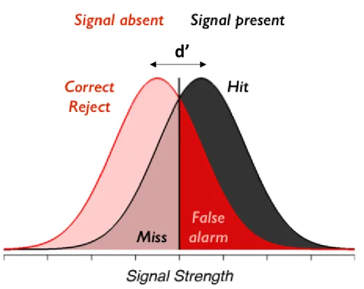
3.1. Signal Detection Theory (SDT) ... 45
3.2. Psychophysical Methods ... 48
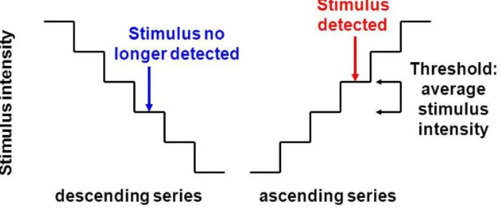
3.2.1. The method of limits ... 48
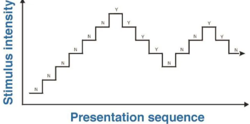
3.2.2. The staircase method ... 49
3.2.3. The method of constant stimuli ... 50
3.3. Psychophysical decision types ... 52
3.4. Psychophysical tasks ... 54
3.4.1. Reaction time tasks ... 54
3.4.2. Simultaneity Judgement tasks ... 54
3.4.3. Temporal Order Judgement tasks ... 56
3.4.4. Temporal Reproduction tasks ... 57
3.4.5. Synchronisation-Continuation tasks ... 58
3.5. Weber’s Law ... 59
3.6. Curve Fitting – The Psychometric Function ... 60
4. Investigating Sensory Timing using Psychophysics ... 65
4.1. The influence of sub and supra-second stimuli on timing ... 65
4.2. Experimental features influencing performance ... 67
4.3. The influence of stimulus presentation order in 2AFC tasks ... 67
x
4.5. The influence of response structure on temporal reproduction ... 69
4.6. Notable considerations for the investigation of duration perception. . 69
4.7. Distinguishing empty and filled intervals ... 70
4.8. Support for centralised timing mechanisms ... 76
4.9. Support for distributed timing mechanisms ... 77
4.10. Neural differences across the senses ... 80
4.11. Timing in clinical populations ... 80
4.12. Other considerations: Samples and their size ... 82
5. Assessing the modality-specificity of the rhythm after-effect ... 86
5.1. Cross-modal influences on rate and duration perception ... 87
5.2. Modality-specific constraints on sub and supra-second duration perception ... 88
5.3. The centralised versus distributed debate... 89
5.4. Methodology ... 91
5.5. Results ... 95
5.6. Discussion ... 109
6. Sensory rate perception – Simply the sum of its parts? ... 118
6.1. The evolutionary basis of rhythm ... 118
6.2. Differences and similarities between duration and rate perception . 119 6.3. Methods ... 123
6.4. Results ... 127
xi 7. Dissociating rhythm and interval discrimination through unimodal temporal
pattern adaptation ... 144
7.1 Interval discrimination and the Multiple Look Model ... 144
7.2. Different types of temporal sequences ... 145
7.3. Neural basis behind anisochrony ... 146
7.4. Temporal irregularity and the senses ... 149
7.5. Factors affecting sequence perception ... 151
7.6. Methods ... 153
7.7. Results... 158
7.8. Discussion ... 167
8. Adapting to cross-modal rhythms in search of a centralised timer ... 172
8.1. Internal representation of cross-modal markers ... 172
8.2. Influence of sensory modalities in empty interval duration discrimination ... 173
8.3. Comparing unimodal versus cross-modal intervals ... 175
8.4. Neurophysiological investigations of cross-modal interval perception ... 176
8.5. Influences of training on cross-modal duration discrimination ... 177
8.6. Methods ... 178
8.7. Results... 184
8.8. Discussion ... 197
xii 9.1. Conclusions ... 211 9.2. Future Work ... 211 10. References ... 215 Appendices Appendix A ... 247
Appendix B: Adjusted p-values for all subjects across all conditions for Experiment 1 in Chapter 5 ... 248
Appendix C: Average amplitudes of effect across all unimodal conditions for each subject for Experiment 1 in Chapter 5 ... 249
Appendix D: Average spread of effect across all unimodal conditions for each subject in Experiment 1 in Chapter 5 ... 250
Appendix E: Holm-Bonferroni-adjusted p-values for all subjects across all conditions for the control experiment in which subjects were unaware of the test modality ... 251
Appendix F: Average amplitudes of effect across both unimodal conditions for each subject from first control experiment in Chapter 5 ... 252
Appendix G: Average spread of effect across both unimodal conditions for each subject from the first control experiment in Chapter 5 ... 253
Appendix H: Table of results from Control Experiment 2 in Chapter 5... 254
Appendix I: Table of results from Experiment 1 in Chapter 6 ... 255
Appendix J: Table of results from Experiment 1 in Chapter 7 ... 256
Appendix K: Table of results from Experiment 2 in Chapter 7 ... 257
xiii Appendix M: Table of results from Experiment 8.3 ... 259
xiv List of Figures
1. Introduction to Sensory Systems and Perception
Figure 1.1 Anatomy of the eye ... 1
Figure 1.2. Schematic demonstration of the human visual pathway ... 2
Figure 1.3. Low and high spatial frequency sine wave gratings ... 4
Figure 1.4. Standard contrast sensitivity function curve ... 5
Figure 1.5. Key structures of the outer, middle and inner human ear ... 7
Figure 1.6. Threshold of normal human hearing plot ... 9
Figure 1.7. Human homunculus ... 13
2. Introduction to Time Perception and Timing Models Figure 2.1. Schematic demonstrating the neural mechanisms of timing ... 23
Figure 2.2. The striatal-beat frequency model ... 25
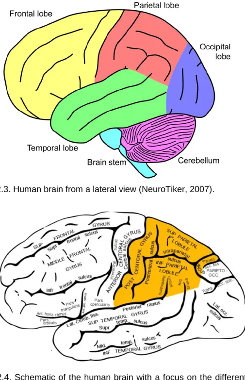
Figure 2.3. Human brain from a lateral view ... 36
Figure 2.4. Schematic of the human brain with a focus on the different structures within the parietal lobe ... 36
Figure 2.5. Example of spatial frequency adaptation ... 42
3. Methodology Figure 3.1. Probability density functions for the signal detection theory ... 46
Figure 3.2. Examples of ascending and descending series in the method of limits ... 49
xv
Figure 3.4. Standard psychometric function ... 51
Figure 3.5. A typical psychometric function as generated from a yes/no detection task ... 53
Figure 3.6. Different stimulus presentation orders in a simultaneity judgement task ... 55
Figure 3.7. A typical simultaneity judgement task ... 56
Figure 3.8. A typical psychometric function ... 60
4. Investigating Sensory Timing using Psychophysics Figure 4.1. The difference between an empty and filled interval of the same temporal length ... 70
5. Assessing the modality-specificity of the rhythm after-effect Figure 5.1. Centralised versus distributed timing mechanism ... 86
Figure 5.2a and 5.2b. Tactor and response disk (respectively) ... 93
Figure 5.3. Schematic simplifying the experimental set-up described ... 94
Figure 5.4. Subject DW’s responses for the unimodal visual condition ... 96
Figure 5.5. Subject DW’s responses for the visuo-tactile cross-modal condition 97 Figure 5.6. All cross-modal and unimodal plots from subject AM ... 99
Figure 5.7. All cross-modal and unimodal plots from subject DW ... 100
Figure 5.8. All cross-modal and unimodal plots from subject YL ... 101
Figure 5.9. Data from the control experiment using the auditory/visual pairing (subject DW) ... 105
Figure 5.10. Data from the control experiment using the auditory/visual pairing (subject AM) ... 106
xvi Figure 5.11. Data from the control experiment using the auditory/visual pairing (subject YL) ... 107 Figure 5.12. Data for all four adapt/test stimulus pairings for subject DW where stimuli were spatially and temporally overlapped ... 110 Figure 5.13. Data for all four adapt/test stimulus pairings for subject AM where stimuli were spatially and temporally overlapped ... 111
6. Sensory rate perception – Simply the sum of its parts?
Figures 6.1a-d. Results from interval reproduction methods after adapting to empty intervals ... 128 Figures 6.2a-d. Results from 2AFC methods after adapting to empty auditory intervals ... 130 Figures 6.3a-f. The after-effect of adapting to different temporal rates
demonstrated through interval reproduction ... 132 Figures 6.4a-f. The after-effect of adapting to different temporal rates
demonstrated through 2AFC ... 134 Figure 6.6. A comparison of temporal rate and single intervals ... 136 Figures 6.7a-f. The after-effect of adapting to different temporal rates
demonstrated through interval reproduction for filled intervals ... 137
7. Dissociating rhythm and interval discrimination through unimodal temporal pattern adaptation
Figure 7.1. An example of local and global anisochrony ... 146 Figure 7.2. Schematic demonstrating an example trial where the subject is
exposed to an anisochronous adapting sequence ... 153 Figure 7.3. Schematic depiction of a temporally regular versus a temporally offset anisochronous sequence ... 155
xvii Figures 7.4a-7.6f. Auditory, tactile and visual baseline pre- and post-adaptation data for all subjects from Experiment 1 ... 159-161 Figures 7.7a-i. Auditory, tactile and visual post-adaptation data for all subjects from Experiment 2 ... 165
8. Adapting to cross-modal rhythms in search of a centralised timer
Figure 8.1. Schematic of the second (interval reproduction) task ... 181 Figures 8.2a-f. Effects of adapting to a 1.5Hz unimodal rhythm through interval reproduction of a 333ms interval ... 186 Figures 8.3a-c. Effects of adapting to a 3Hz audio-visual rhythm demonstrated through interval reproduction of a 500ms empty interval ... 188 Figure 8.4. Comparison of non-co-localised after-effect ... 189 Figures 8.5a-c. After-effect of adapting to a co-localised 3Hz audio-visual rhythm ... 191 Figure 8.6. Comparison of co-localised after-effect ... 192 Figures 8.7a-c. 2AFC cross-modal versus unimodal rhythm matching ... 195-196
xviii List of Tables
5. Assessing the modality-specificity of the rhythm after-effect
Table 5.1. Adjusted p-values for all subjects across all conditions ... 102 Table 5.2. Average amplitudes of effect subject ... 102 Table 5.3. Average spread of effect ... 103 Table 5.4. Holm-Bonferroni-adjusted p-values for all subjects for first control experiment ... 107-108 Table 5.5. Average amplitudes of effect across both unimodal conditions for each subject ... 108 Table 5.6. Average spread of effect across both unimodal conditions for each subject ... 108 Table 5.7. Amplitudes (μ) and spread (σ in log units) of adaptation effect and Holm-Bonferroni-adjusted p-values for each subject for the second control
experiment ... 112
6. Sensory rate perception – Simply the sum of its parts?
Table 6.1. Results from experiment 1 for subjects AM and DW with 95%
confidence intervals ... 131
7. Dissociating rhythm and interval discrimination through unimodal temporal pattern adaptation
Table 7.1. 95% Confidence interval values and standard error values ... 162-163 Table 7.2. 95% Confidence interval values and standard error values ... 166
xix 8. Adapting to cross-modal rhythms in search of a centralised timer
Table 8.1. Paired-samples t-test from Experiment 8.2 ... 189-190 Table 8.2. Paired-samples t-test from Experiment 8.3 ... 193
xx List of Abbreviations
LGN Lateral Geniculate Nucleus
V1 Visual Cortex
MLE Maximum Likelihood Estimation
SBF Striatal Beat-Frequency
tRNS transcranial Random Noise Stimulation IPL Inferior Parietal Lobule
SMG Supra Marginal Gyrus
SMA Supplementary Motor Area
MEG Magnetoencephalography
SDT Signal Detection Theory
2AFC Two-Alternative Forced Choice
SOA Stimulus Onset Asynchrony
PSE Point of Subjective Equality
TOJ Temporal Order Judgement
JND Just Noticeable Difference ITD Inter-aural Time Difference
ERP Event-Related Potential
CRF Clinical Research Facility
A Auditory
T Tactile
V Visual
1 1. Introduction to Sensory Systems and Perception
1.1 Visual Perception
Visual perception is perhaps one of the most important functions humans have evolved through time, and in an increasingly visual society, this system remains fundamental to not only our survival but also our quality of life. The visual system detects and interprets light signals to build a perceptual representation of the physical world. Anatomically, it is mediated through a system consisting of retinal photoreceptor cells, the optic nerve and optic chiasm, lateral geniculate nucleus (LGN), optic radiations, and V1 (also known as the primary visual cortex/striate cortex). Higher levels of the visual system include areas V2, V3, V4 and V5/MT in mammals. The following chapter will elaborate on these structures in more detail.
Figure 1.1. Anatomy of the eye, (Hejtmancik & Nickerson, 2015).
Light enters the eye and is refracted via the cornea (Figure 1.1). On passing through the pupil it is then further refracted by the lens and an inverted image is then projected to the retina. The retina contains a large number of receptor cells called
2 rods and cones (and collectively referred to as photoreceptor cells). Photoreceptors remain crucial to our visual abilities as photoreceptor proteins absorb photons, activating a change in the cell’s membrane potential and stimulating biological processes. This action represents the process of transduction (Goldstein, 2007). Strictly, the retina contains three different types of photoreceptor cells – rods, cones and photosensitive retinal ganglion cells. Rods and cones are understood to directly contribute information to build a representation of the world whereas photosensitive retinal ganglion cells (discovered much more recently) are thought to not directly contribute to vision but support pupillary reflexes and circadian rhythms (Berson, Dunn, & Takao, 2002). Rods are extremely sensitive to light and are therefore the driving photoreceptor in environments with low light levels (as colour vision and the contribution from cones becomes less essential). Cones, on the other hand, require a larger number of photons and therefore significantly brighter light to produce a signal. Their primary role includes responsibility for daytime vision and visual acuity (sharpness of vision as they provide us information on fine detail of our environment). Humans possess three different types of cone cells, each responsible for a different wavelength of light (of short, medium and long wavelengths) and the ability to perceive colour is deduced by evaluating these signals. It is understood that, on average, the human retina possesses 120 million rods and 6 million cones (Osterberg, 1935).
3 Figure 1.2. Schematic demonstration of the human visual pathway (Nieto, 2015). The optic nerve then transmits information about the retinal image to the optic chiasm, a cross-shaped structure (Figure 1.2). Here, information from both eyes is amalgamated and split according to visual field. The corresponding half fields of views are contralaterally sent to those halves of the brain to be processed (so information from the right field of view of both eyes is sent to the left half of the brain and information from the left field of view of both eyes is sent to the right half of the brain to be processed). Both the left and right optic tract (now carrying visual information from contralateral visual fields) continue to the lateral geniculate nucleus (LGN). Neurons in the LGN then transfer the visual image to the occipital lobe and visual cortex where the image is further processed. The primary visual cortex (V1) receives information directly from the LGN and visual information then travels via a cortical hierarchy to higher-processing areas in the cortex.
Areas V1 and V2 are involved in processing basic visual features, as neurons in these regions respond selectively to specific orientation and position, and are believed to process basic information about size and space. Area V3 is involved in shape perception whereas V4 is involved in colour vision. Areas V3 and MT/V5 are involved in motion detection, spatial localisation and hand and eye movements. The complexity of neural responses increases as information passes through the visual hierarchy. For example, where a V1 neuron may selectively respond to a particular orientation, neurons in the visual association cortex may respond selectively to faces. Further specialisation occurs when visual information is split into dorsal and ventral streams (Mishkin & Ungerleider, 1982).The dorsal stream, often referred to as the ‘where’ stream deals with spatial attention. However, this particular area has also been referred to as the ‘how’ stream to demonstrate its influential role in guiding movements towards spatial locations (Goodale & Milner, 1992). Conversely, the ventral stream is known more commonly as the ‘what’ stream as it is involved in acknowledging and categorizing visual input. Whilst substantial documentation exists supporting these two visual streams, there still exists some debate as to how
4 independent they are as there exists a substantial cross-over between the two streams.
Central to our visual abilities are the contrast sensitivity and visual acuity functions. Contrast is specifically the change in luminance over the overall luminance level (∆L/L). Contrast sensitivity is the log of the aforementioned function, and is understood as the detection of minimal luminance levels of an object of visual focus (compared to its respective background) (Figure 1.4) (Amesbury & Schallhorn, 2003).
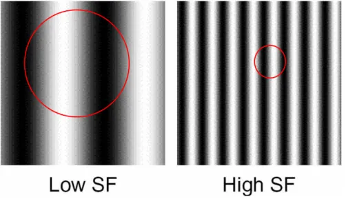
Figure 1.3. Low and high spatial frequency sine wave gratings. (New York University
Website, retrieved 20 September, 2016, from
http://www.cns.nyu.edu/~david/courses/perception/lecturenotes/channels/channel s.html, (Landy, 2006)). A sinusoidal grating consists of light and dark bars, the intensity of which is determined by the sine function in trigonometry. The red circles indicate the centre and surrounding concentric areas (see text for further description).
5 Figure 1.4. Standard contrast sensitivity function curve; visual acuity is a single point on the contrast sensitivity function (Emergent Techniques for Assessment of Visual Performance, National Research Council, 1985; Campbell & Robson, 1968). The red cross represents visual acuity.
Two examples of low and high spatial frequency gratings can be seen in Figure 1.3. Retinal ganglion cells located most centrally in the fovea are known to have the smallest receptive field sizes. Contrastingly, retinal ganglion cells with the largest receptive fields are located in the visual periphery. Receptive field sizes are of incredible importance as they ultimately govern the spatial frequency of visual input. High spatial frequencies (fine detail) stimulate small receptive fields whereas low spatial frequencies (coarse detail) stimulate large receptive fields. Typical receptive fields of retinal ganglion cells consist of two concentric areas (Figure 1.3), known as the centre and surround. These areas perform antagonistically, in simpler terms, light falling on the central area excites the neuron whereas light falling on the surround inhibits the same neuron. When the level of excitation exceeds the level of inhibition, the neuron will cause an action potential to travel down its axon. Figure 1.4 depicts a contrast sensitivity function. The highest visual sensitivity falls between the range of moderate spatial frequencies (around 1-5 cycles/per degree) and thus
6 sensitivity for spatial frequencies above and below this range decreases. The highest spatial frequency visible indicates visual acuity. Visual acuity refers to the sharpness of retinal function in central vision (Hofstetter, Griffin, & Cline, 1997). Simply put, visual acuity describes the ability to see high contrast detail in central vision. One method of measuring visual acuity is using the Snellen chart, where individuals are required to centrally fixate on examples of stylized letters from a fixed distance (known as optotypes). An alternative measure of visual acuity could also present Landolt rings instead of letters. However, a more reliable form of measurement is using logMAR visual acuity charts as these charts typically contain more letters than a Snellen chart. Each row on a logMAR chart contains 5 letters, and each row has a step of 0.1 log units between the next row. The value assigned to each individual letter is 0.02 log units. An individual’s logMAR score is thus the total of each letter correctly read. A 6/6 measurement on a Snellen chart is equivalent to a 0.0 logMAR score (Elliott & Flanagan, 2007). The main advantages of LogMAR charts is that the letter size varies logarithmically between lines so is standardised, as is the letter legibility. Additionally, as the logMAR scoring method accounts for each letter, it allows for more reliable and precise measurements of VA compared to simply deducing a score from each line alone (Bailey, Bullimore, Raasch, & Taylor, 1991).
The visual system is not passive and instead is continually adaptive to changes in sensory information. Accordingly, it adjusts to accommodate for these changes (more commonly known as neural adaptation). Demonstrations of such adaptive mechanisms include motion after-effects, orientation after-effects, and negative afterimages (Barlow & Hill, 1963). The motion after-effect is thought to be a result of motion adaptation; whereby after viewing a moving visual stimulus with stationary eyes, fixating on a stationary image results in the perception of motion in the opposite direction, (with respect to the direction of the initial stimulus presentation). Visual adaptation more specifically occurs as responsiveness to a constant visual stimulus changes over time within sensory systems. Notably, visual adaptation can occur for a variety of visual features, such as orientation, motion and spatial frequency; and is thought to occur to establish coherence of the sensory world, and
7 maintain perceptual constancy (Webster, 2015). Neural adaptation will be expanded upon and explored further in Chapter 2.
1.2 Auditory Perception
The ability to perceive sounds is known as auditory perception. This occurs through a detection of vibrations and changes in pressure of the surrounding medium (for example, air or water, through time).
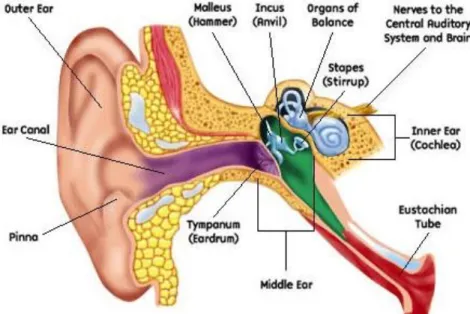
In humans, hearing is performed by the auditory system where vibrations are detected and transduced into nerve impulses by the ear. These nerve impulses are then translated by the temporal lobe and communicated to other areas of the brain. To elaborate on the precise mechanisms underlying hearing and auditory perception, it is essential to understand the three components of the human ear; the outer, middle and inner ear(s) (Figure 1.5).
Figure 1.5. Key structures of the outer, middle and inner human ear. (Hearing Haven
website, retrieved 21 September 2016, from
8 The outer ear corresponds to the visible part of the ear and the ear canal terminating at the ear drum. This part of the ear also includes the pinna – a structure that helps focus sound waves through the ear canal and in the direction of the ear drum. The structure of the ear drum is that of an airtight membrane and therefore, as sounds arrive in this location, they cause the membrane to vibrate. It is also noteworthy to consider that due to the asymmetrical nature of the outer ear, the location the sound is arriving from will dictate how the sound is filtered. The middle ear contains an air-filled chamber within which are three of the smallest bones in the body (known collectively as the ossicles) and individually as the malleus, incus and stapes. These structures help transmit vibrations from the ear drum towards the inner ear. Lastly, the inner ear contains the cochlea, a spiral-shaped, tube-like structure which contains the organ of corti. This incredible receptor organ allows for the translation of auditory signals into action potentials. Specifically, this occurs when vibrations to the structures of the inner ear cause cochlear fluid to displace and create movement of the hair cells at the organ of corti to produce electrochemical signals. In this way, the organ of corti is essential to allow mechanotransduction in the inner ear and thus, allows for the cortical and cognitive understanding of sound.
Information from the cochlea then travels through the auditory nerve towards the cochlear nucleus in the brainstem. These signals are then projected to other areas of the brain, such as the inferior colliculus, which then integrates this sound information with input from other areas of the brain and allows for subconscious reflexes. The inferior colliculus also projects to parts of the thalamus such as, the medial geniculate nucleus where this sound information is further communicated to the primary auditory cortex located in the temporal lobe. The primary auditory cortex also holds Wernicke’s area, an area believed to help interpret the sounds necessary to identify and comprehend spoken words.
As experienced with other senses, the auditory system is not immune to limits; and understandably, there exist some general limitations to human audition. The first of these is in what can actually be heard by humans. Whilst the threshold for detection of frequencies substantially increases with age (meaning lower frequencies can
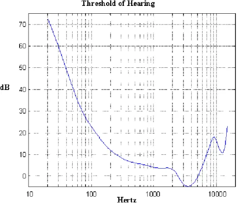
9 often go unheard), most young and healthy adults can detect frequencies between 20-20,000Hz (Figure 1.6). In terms of an absolute threshold of hearing (meaning the lowest energy physically detectable), it has been found that this absolute threshold of detection depends greatly on the frequency of noise being perceived. A comparative analysis conducted in 1979 suggests that the lower limit of perception lies at -5dB rather than 0dB. However, the authors note that whilst this threshold has been documented, it is incredibly rare and for the majority of people the threshold lies between 0 and 5dB (Robinson & Sutton, 1979).
Figure 1.6. Threshold of normal human hearing plot. As auditory perception is influenced by the frequency of signals, the y-axis represents the auditory intensity required for hearing (in decibels), whereas the x-axis represents the frequency of signal presentation (in Hz). From ISO, R. (1987). 226: Normal equal-loudness contours for pure tones and normal threshold of hearing under free field listening conditions. International Organization for Standardization, Geneva.) (Acoustics—
10 Even in individuals whose hearing falls within ‘normal’ clinical thresholds, differences in temporal perception bound to intrinsic individual differences can exhibit themselves. Furthermore, despite neurotypical cochlear neuropathy (Shinn-Cunningham, Varghese, Wang, & Bharadwaj, 2017), differences manifest through physiology and behaviour in individuals with “normal” hearing can present as a result of auditory nerve fibre differences that typically respond to sound (Shinn-Cunningham et al., 2017).
1.3 Tactile Perception
Tactile perception refers to the sense of touch. This ability depends on the somatosensory system – an incredibly complicated network of nerve cells, which respond selectively to particular changes - to both the surface being touched and also the internal state of the body. A collection of nerve cells also known as sensory receptors communicate signals along to the spinal cord where these signals can be processed by other nerve cells and later, sent to the brain for extended processing. Such sensory receptors are found all along the surface of the body even in internal tissue, such as the epithelial tissue, skeletal muscles and the cardiovascular system. Thus, the somatosensory system is composed of both sensory receptors and afferent neurons that send signals towards neurons located in the central nervous system.
Broadly, the somatosensory system is a three-order neuronal system that communicates detected sensations peripherally and, using pathways through the spinal cord, brainstem and thalamic relay nuclei, conveys sensory information to the sensory cortex located in the parietal lobe. Receptors carry sensory impulses through sensory afferents to the dorsal root ganglia, where cell bodies of the first order neurons are located. These then travel through to the spinal cord, either ipsilaterally or contralaterally. The spinal cord contains neurons of the second-order fibres containing information regarding pain, touch and temperature sensations. Fibres for second-order neurons containing information regarding touch, position and vibratory sensations are held within the medulla. These fibres are then conveyed either to the thalamus or the cerebellum. The thalamus is the location of
11 third-order neurons. The thalamic nucleus then transports sensory afferents to cortical sensory areas where this information is organised and analysed in an incredibly sophisticated manner.
Whilst sensory receptors are characterised by their ability to identify changes in their immediate periphery, these receptors are also crucially able to adapt to a variety of stimulus features. Specifically, this means they are able to reduce and control their rate of discharge resulting from continuous or repetitive stimulation. Receptors possessing this quality initially respond maximally as the stimulus is experienced, however as continuous stimulation is experienced, this response begins to fade, resulting in effects of adaptation as experienced in other senses such as vision and audition also. It is important to note here that not every sensory receptor holds the ability to adapt to evolving stimulus features and therefore, nonadaptive sensory receptors actually respond continuously for the duration of the stimulus being responded to.
Further specialisation within the somatosensory system occurs depending on the exact type of touch being experienced, explicitly whether this is fine or crude touch. Fine touch, also known as discriminative touch, allows for the identification of the location of the touch. Crude touch on the other hand, is where identification of touch exists however awareness of the exact location of touch is unavailable. Processing of fine touch typically occurs in the posterior (dorsal) column-medial lemniscus pathway which then sends information regarding the fine touch to the cerebral cortex. Processing of crude touch information on the other hand, occurs in fibres located in the spinothalamic tract. A subject will be able to discriminate fine touch so long as the fibres in the posterior column-medial lemniscus pathway operate as normal. As soon as these fibres are severed or disrupted, whilst the subject will still be able to discriminate touch, they will not be able to gauge the precise location of this touch and therefore, will be reduced to experiencing crude touch only.
A classic task used to investigate thresholds for tactile perception is the two-point discrimination task. This task asses the ability to gauge that two closely placed objects are touching the skin at two different points rather than confusing them for
12 one. The test is usually conducted on a range of areas on the surface of the skin to better understand how densely innervated that particular location of skin is. Whilst this is an incredibly traditional task, it has been criticised on occasions for poor resolution of spatial-tactile acuity. Demonstrations of the task showing low sensitivity and understating sensory deficits or even failing to detect them have all been documented (Van Boven & Johnson, 1994; van Nes et al., 2008). In response to these criticisms, a number of alternative tasks have been implemented to test ‘pure’ spatial-tactile acuity – examples of these include the grating orientation task, the raised letter task and the two-point orientation discrimination task (Craig, 1999; Vega-Bermudez & Johnson, 2001; Tong, Mao, & Goldreich, 2013). As these tasks require the subject to identify the spatial nature of the perceived sensations in an absence of response magnitude clues, for example, identify the exact spacing of the two-points and their orientation rather than simply stating whether they were felt or not, researchers have begun to implement them more often in tactile research (Johnson & Phillips, 1981; Tong et al., 2013).
Wilder Penfield has created a cortical map of body surfaces in the brain (called the ‘homunculus’ depicted below (Figure 1.7)). It is important to note that whilst this map presents an incredibly useful understanding of the representation of bodily areas cortically, it is still susceptible to change and reports of substantial plasticity exist in subjects who have experienced significant injury or stroke (Borsook et al., 1998).
13 Figure 1.7. Human homunculus indicating physical bodily areas and areas they correspond to cortically (Penfield & Rasmussen, 1950).
On a final note, the somatosensory system is not immune to limits of perception either. Sensory neurons are not distributed uniformly amongst the surface of the skin; in other words, some areas such as the fingers are more densely populated with sensory neurons compared to others such as the back. It is due to this feature that discrimination of different tactile sensation is different depending on the area stimulated. For a minority of individuals, deficits in being able to perceive objects through touch also exists. These individuals are unable to categorize objects in a tactile sense, and this deficit is thought to result from damage or lesions to the somatosensory cortex, termed astereognosis.
1.4 Principles underlying multisensory perception
The purpose of sensory systems is to guide adaptive behaviour. Multisensory processing is the function that deals with how sensory modalities interact, combine and influence processing. It is wholly reliant upon abilities of the nervous system to incorporate and integrate information from numerous modalities. Crucially, not only
14 does multisensory integration allow us to have meaningful perceptual experiences but also maintains perceptual constancy, and is therefore central to adaptive behaviours. Whether groups of temporally coincident sensory signals are to be integrated or segregated is based on the congruence of those sensory signals. Sensory signals can be categorised by their modality (for example, is the stimulus visual or auditory?), the spatial location of the sensory signals (for example, are the signals arriving from the same physical location or separate locations?), and duration of the signals (for example, are they present for the same amount of time). Stein and Meredith have postulated three principles which multisensory integration appears to observe (Stein & Meredith, 1993):
1) The Spatial Rule: Successful multisensory integration is more likely when unimodal sensory stimuli arise from approximately the same spatial location. 2) The Temporal Rule: Successful multisensory integration is more likely when
unimodal sensory stimuli occur at approximately the same time.
3) The Principle of Inverse Effectiveness: Multisensory stimuli are more successfully and effectively integrated when the alternative, unisensory response is comparatively weak.
In support of these principles, data from experimental studies show that subjects typically respond faster to multisensory stimuli compared to the same stimulus presented in isolation (Hershenson, 1962), and to double targets where two (unrelated) targets are presented simultaneously compared to being presented in isolation (Ridgway, Milders, & Sahraie, 2008).
Numerous studies have also indicated the dependence of integration upon several low-level and high-level factors (Radeau & Bertelson, 1977; Welch & Warren, 1980; Welch, 1999; Spence, 2007; Vatakis & Spence, 2007, 2008, 2010). Low level factors refer to temporal information such as temporal synchrony and temporal correlations between modalities and also information regarding spatial locations (Chen & Vroomen, 2013), whereas high-level factors refer to prior knowledge and semantic congruency (Doehrmann & Naumer, 2008). A well-established view amongst
15 researchers in this field of a theory that combines both factors is that of the “assumption of unity” – as information from multiple modalities share more (amodal) properties, the more likely it is that they will be integrated as the brain understands them as originating from a common source (Bedford, 1989). The most crucial amodal property then, is that of temporal coincidence (Radeau, 1994). Only when information from two different sense organs arrives in the brain at the same time are events thought to be considered as multisensory in nature, otherwise two separate amodal events are thought to occur rather than one multisensory event (Keetels & Vroomen, 2012). Constructing a clear and definitive picture of multisensory temporal processing is indeed problematic as the brain has no distinct sense organ that registers time on an absolute scale. In addition, to successfully perceive synchrony the brain has to process differences in physical and neural transmission times, in other words, naturally occurring lags in arrival times and processing times of the different information streams. It is noteworthy that these times also differ for different senses. Ultimately, intersensory timing is flexible and adaptive, however in efforts to deal with various lags between the senses the brain employs a variety of different methods:
1) Manipulating a window of temporal integration 2) Compensation for external factors
3) Temporal recalibration 4) Temporal ventriloquism
Specifically, the first hypothesis suggests that processing systems may be dismissive of small temporal delays between stimulus presentations and therefore, manipulate this window of temporal integration by increasing its duration. The second hypothesis suggests that an incorporation of external factors and previous world experiences may help form coherency in asynchronous presentations of multisensory stimuli, for example, even though in conversation, our ability to observe lip movements and their corresponding sounds may not coincide, our understanding that the two correspond to the same social event may enable us to maintain perceptual constancy. Temporal recalibration refers to the ability of sensory systems
16 to actively alter subjective simultaneity in multisensory signals to perceptually reduce discrepancies between the two and maintain the perception of simultaneity. The final hypothesis refers to an ability to shift the perceived timing of a specific sensory stimulus towards that of another modality, such that they may be perceived as having occurred together.
Multisensory integration is thought to occur in a statistically optimal fashion (Hartcher-O'Brien, Di Luca, & Ernst, 2014) where each sensory signal is weighted according to its precision. As an unbiased estimate is produced with the highest possible precision, this results in a statistically optimum approach (Hartcher-O'Brien et al., 2014). A note should also be made of the ‘Modality Appropriateness Hypothesis’ (Welch & Warren, 1980). Welch and Warren have used this theory to explain how in situations of sensory conflict and uncertainty, the modality most reliable and fitting for the occasion becomes the one to dominate perception; thus, different senses contribute differentially to sensory integration depending on how reliable and appropriate they are, given the task at hand (Welch & Warren, 1980). The Modality Appropriateness Hypothesis explains that in situations dealing with the spatial localisation of stimulus, vision has a greater influence than audition and similarly, in situations dealing with explicit timing, audition has a presence that overrides vision (Welch, DutionHurt, & Warren, 1986). The critical importance of reliability in multisensory perception has also been extended to Bayesian Integration (Ernst & Banks, 2002), who suggest cue combination occurs by utilising the maximum likelihood estimation (MLE) principle. Each sensory signal is associated with its own noise value (due to noise in physical environments and internal conditions, such as inherent noise in internal transmission for example, from spontaneous neural firing) (Ernst & Bulthoff, 2004). The MLE principle deals with minimising uncertainty by combining multiple observations and the noise associated with each observation and associating heavier weightings to the more ‘reliable’ signals. The perceptual decision is then dominated by the estimate with the lowest variance. Sensory information being integrated in this way increases the reliability of the estimates and delivers the “most reliable unbiased estimate” available (Ernst & Bulthoff, 2004).
17 In summary, sensory systems differ vastly on how they perceive temporal events depending on the time taken to receive and process the range and variety of sensory signals. Our brains intuitively combine signals from multiple senses when those signals are presented in close temporal or spatial proximity (Deroy & Spence, 2016), and it has been noted that multiple senses increase the likelihood of veridical perception of the real world (Stein & Meredith, 1993; Ernst & Bulthoff, 2004). Indeed, the causal origin of cross-modal signals is perhaps one of the most important determinants of multisensory binding (Deroy & Spence, 2016). Other notable features of multisensory binding include bi-directionality, for instance, if vision can influence audition then audition can also influence vision. Many of these cross-modal relationships are shared across cultures (Athanasopoulos & Moran, 2013) and some are even considered universal (Deroy & Spence, 2016). A question currently undergoing intense study is how temporal signals from each modality are weighted (Hass, Blaschke, & Herrmann, 2012). The Modality Appropriateness Hypothesis suggests that only the most reliable modality would be picked to contribute an estimate of time, and consequently, estimates from less reliable modalities would not be used. The Bayesian Integration alternative however, posits that weights are assigned according to the reliability of each modality, thus incorporating all available sources of information to combine an estimate of time (Deneve & Pouget, 2004).
1.5 Neural correlates of multisensory integration
Results from brain imaging studies implicate the posterior medial frontal and insular cortex to be importantly activated in the timing of visual and auditory stimuli, whereas the MT/V5 has been suggested to be necessary for the timing of visual events only. It appears plausible that because multisensory perception and integration involve a multitude of cortical areas, the neural correlates of such abilities will also be (predictably) distributed across multiple neural areas. Future work should aim to further classify the distinct areas responsible for processing multisensory input under a comprehensive and extensive range of environments.
19 2. Introduction to Time Perception and Timing Models
Time is a dynamic quality fundamental for existence. In demonstrating its importance for survival it is known that almost all plants and animals – even unicellulars, have been documented to express circadian rhythms (Arechiga, 1996). Of note is also the fact that the ability to perceive time does not stand alone – whereas space has high perceptual availability, time, on the other hand, is transient and constantly fleeting - we can go back and check a map – this act, however, is impossible to do with time. Furthermore, as we lack a specialised organ to process time, our awareness of time is solely derived from our sensory systems. These too however, are not without their complications. For example, very few instances in life are purely unisensory (for example, rainbows) – most are multi-modal (for example, speech) requiring an integration of multiple sensory signals. Collectively, this means that our sense and processing of time is dependent upon a range of sub-systems processing sensory input intertwined with temporal signals. These influencing factors and intricacies are what make the study of time incredibly exciting, but complex. For example, temporal processing capacity has been thought to be influenced by a range of different factors, including (but not limited to), sensory modality, stimulus complexity, linguistic demands and combinations of various intensities of these. Deficits in visual temporal processing have been hypothesised to underlie impairments in dyslexic adults (Meyler & Breznitz, 2005). Despite being a fundamental component to physics and philosophy enthralling scientists and philosophers alike for millennia (Muller & Nobre, 2014), we understand very little about this feature, and have made only incremental progress on the subject of temporal processing in humans.
2.1 Models of Time Perception
Interestingly, despite our sense of time providing a foundation to other abilities such as motion perception and action, our sense of time is regularly far from veridical (Shi
20 & Burr, 2016). Shi and Burr suggest that a combination of adaptive recalibration and minimised predictive errors constitute the human sense of subjective time, suggesting that perception is an inference of sensory stimulation (Shi & Burr, 2016). They further suggest that our sense of time is unique in that it does not arise from a specific or even physical organ, and that all sensory signals contain temporal cues, irrespective of the modality they are presented to. The “heterogeneous” manner of processing is what creates disparities for subjective time across the range of sensory modalities that humans possess. Several lines of evidence support the idea that time is processed differentially depending on the combination of durations and modalities, namely:
Psychophysical and psychopharmacological experiments both postulate the presence of distinct mechanisms underlying temporal measurements, for instance, Weber’s Ratio – the coefficient of variation, is different for durations shorter and longer than 2 seconds (Gibbon, Malapani, Dale, & Gallistel, 1997).
Dopaminergic and cholinergic antagonists differentially affect the temporal processing of short (<1 second) and long (>1 second) durations (Rammsayer, 1999).
Interval discrimination is significantly worse between modalities, compared to within modalities (Grondin & Rousseau, 1991).
In perceptions of duration, sounds are consistently perceived as longer in duration compared to perceptions of lights (Wearden, Edwards, Fakhri, & Percival, 1998).
It has been recorded that the auditory cortex appears to have a more profound effect on temporal discrimination on not only auditory stimuli but also visual stimuli. The asymmetric contributions of visual and auditory cortices in time perception have been explained by the remarkable aptitude of the auditory system in timing (Kanai, Lloyd, Bueti, & Walsh, 2011).
Broadly, the perception of time has been split into two schools of models – dedicated and intrinsic models. The former deals with theories presenting mechanisms where
21 time is explicitly and deliberately coded by cortical systems. On the other hand, the latter refers to theories suggesting that time is encoded as an emergent property of neural dynamics (for example, state-dependent networks, which will be expanded on below) (Spencer, Karmarkar, & Ivry, 2009). The following subsections will elaborate on the most comprehensively developed models of time perception. 2.2 Pacemaker-Accumulator Model and Scalar Expectancy Theory
It has been postulated that there is one internal clock that underlies all human timing judgements (Treisman, 1963). Specifically, it has been suggested that this internal clock primarily deals with the function of transforming a period of objective time into subjective time (Allman et al., 2014). Whilst the neural bases for either the pacemaker or accumulator are unknown, they are suggested to have a link with cerebral oscillations (Nagarajan, Blake, Wright, Byl, & Merzenich, 1998).
Within this internal clock model, it is suggested that a pacemaker mechanism exists which emits a series of crucial pulses. When an interval is to be calculated, a trigger switch is activated by the onset of that interval which then allows the counting process to begin, allowing the accumulator to count the total pulses during the interval (Zakay & Block, 1997) and the duration to be estimated from the total count of pulses. The number of pulses emitted during a certain time frame are counted by an ‘accumulator’ which then determines temporal frames. The pacemaker-accumulator model suggests a separate pacemaker for each modality (Hass, Blaschke, Rammsayer, & Herrmann, 2008), these pacemakers emit pulses at particular frequencies which are then modulated by events in that modality (Brown, 1995; Kanai, Paffen, Hogendoorn, & Verstraten, 2006; Eagleman, 2008). A centralised temporal hub then counts these pulses. The accumulator hub and the trigger switch are both centralised. When disparity exists between modalities and their independent estimates of time (Gamache & Grondin, 2010), the final estimate can only be contributed to by modalities that contain both the onset and offset estimates. The pacemaker-accumulator model therefore implies that the same clock times signals from multiple modalities. Evidence suggesting asymmetrical influence of multiple modalities on time perception (Hass, Blaschke, & Herrmann, 2012),
22 would need to be addressed and modified by supporters of the model for it to still be considered an appropriate and relevant explanation of human temporal processing.
Akin to pacemaker theories, the Scalar Expectancy Theory also posits that an internal clock dominates human (and animal) timing behaviour. Specifically, that a pacemaker (the internal clock), accumulator and a connecting switch modulate this internal clock. The theory also proposes memory stores and decision mechanisms that help construct timing behaviour. Further, it has been suggested that this pacemaker does not operate on a fixed rate and can modulate its speed bi-directionally. This means the pacemaker can both, accelerate and decelerate for example, in duration adaptation experiments inducing duration overestimation and compression, respectively (Yuasa & Yotsumoto, 2015). In the understanding of an internal clock model, differences in clock speeds for specific modalities can be as a result of differences in the pacemakers for those modalities thus explaining perceptual differences (Yuasa & Yotsumoto, 2015). The scalar property of timing (also called Weber’s Law) refers to the observation that interval timing errors emerge in a linear manner with the interval’s estimated size. This observation has been documented in a number of animals including humans, rodents and pigeons (Gibbon, Malapani, Dale, & Gallistel, 1997; Malapani & Fairhurst, 2002; Buhusi et al., 2009). Despite the support for this theory from animal studies, properties of human timing are undoubtedly more complex and a key reason behind this is due to attentional allocation (Hallez & Droit-Volet, 2017). Moreover, the Scalar Expectancy Theory has dominated the field for decades positing a single centralised and modality-independent clock. This has recently become challenged by the hypothesis of distributed sensory timing mechanisms across several brain areas/circuits and that the recruitment of these mechanisms depends on the psychophysical task at hand, length of temporal intervals and sensory modality (Ivry & Schlerf, 2008; Vicario, Martino, & Koch, 2013; Mioni, Grondin, Mapelli, & Stablum, 2018).
23 2.3 Interval Timing Models
Some of the earliest scientific works using time and specifically, duration reproduction, were conducted by Karl von Vierordt who asked subjects to reproduce an interval between two taps by tapping themselves (Vierordt, 1868) which informed us of principles of perceived duration in relation to physical duration (Lejeune & Wearden, 2009). The intrinsic timing model suggests time is an inherent and largely generalized feature of neural dynamics (Bueti, 2011). This suggests that principally, any area in the brain should, and indeed is, able to process and encode time. A great advantage of these models is that because they assume time is encoded the same way as other stimulus properties are such as motion or colour, they allow for an explanation of the functional organisation of sensory timing mechanisms. However, much of the evidence in support of intrinsic timing models relies on much shorter durations of less than 500ms (Buonomano & Maass, 2009; Spencer et al., 2009). And so, for intrinsic timing models to fully explain sensory timing mechanisms, much larger testing durations are needed (Bueti, 2011).
24 Figure 2.1. Schematic demonstrating the neural mechanisms of timing. a) A specialised timing model posits a specific neural region that is dedicated towards the representation of temporal information. This system is thus recruited when temporal processing is required. The cerebellum is presented as a specialised timing structure in this schematic. b) The distributed timing model posits that temporal information is processed by a symphony of neural structures. c) The local timing model posits that instead of being processed by a dedicated timing mechanism, temporal information is processed by the neural structures recruited by the particular task at hand. Image acquired from Ivry & Spencer, 2004.
It has been proposed that interval-based timers rely on non-oscillatory mechanisms (Wittmann, 1999) where different durations are then processed by dedicated timers specific to those durations localised in the cerebellum (Ivry, 1996). Contrastingly, oscillatory clock-counter systems have been proposed to be localised to the basal ganglia (Wittmann, 1999).
2.4 Oscillatory and Neural Models
2.4.1 Striatal Beat-Frequency Model
Despite having no physical organ, such as those that relate to our perception of colour or sound, our perception of time is no less perceptually salient (Ivry & Spencer, 2004). The physical and biological worlds both provide us with multitudes of oscillatory events. Physical examples include planetary motion in the form of years, seasons and days, whereas biological examples include breathing cycles and heartbeats. Biological clocks can also be entrained to the physical time keepers tracking days and seasons and are present in some of the simplest lifeforms we can examine, such as bacteria, algae and yeast (Fitch, 2012). Entrainment refers to when two or more oscillators become coupled in their activity. Neural entrainment refers to temporal calibration of oscillators within the brain (van Wassenhove, 2016).
25 Cortico-striatal circuits are believed to subserve interval timing under the Striatal Beat-Frequency (SBF) model. The model proposes a bundle of cortical neurons that constantly oscillate at various frequencies, these are accompanied by striatal spiny neurons responsible for detecting patterns of phases within the cortical oscillating neurons. At the onset of an event, cortical oscillating neurons are reset and begin a new cycle of oscillation. These oscillators are linked to different frequencies which then project this information to medium spiny neurons (A and B) located in the striatum, activating if particular patterns of phases are evidenced amongst the oscillators (Figure 2.2). These medium spiny neurons (A and B) then detect oscillating patterns amongst the cortical oscillators – as different oscillators oscillate to different frequencies, by detecting specific coincidental patterns, the spiny neurons are able to code multiple durations (Buhusi & Meck, 2005; Murai, Whitaker, & Yotsumoto, 2016).
Figure 2.2. The striatal-beat frequency model. The top right of the image shows lower frequencies whereas the bottom right of the image shows higher frequencies. The model posits cortico-striatal circuits that allow a neural construction of interval timing. Cortical neurons on the left side of the image oscillate at a number of different frequencies and the neurons on the right of the image (Striatal Spiny Neuron A & B) detect patterns of oscillations amongst the oscillating neurons. As the oscillating
26 neurons have different frequencies, this allows the system to code for different durations (Image courtesy of Murai et al., 2016).
Importantly, the SBF model addresses modality-specific and modality-independent features of timing. This is due to the oscillators being located in multiple areas of the cortex, and this assumption is based on the fact that medium spiny neurons actually receive input from all over the cortex (Cowan & Wilson, 1994). Consequently, these oscillators distributed across the cortex can be modulated within a modality-dependent framework. The coincidence detectors in the form of medium spiny neurons are centrally based in the striatum and therefore modality-independent. This hypothesis is further strengthened by evidence promoting the role of the striatum in multisensory integration (Reig & Silberberg, 2014).
Temporal computations that are state-dependent propose that performance of neural dynamics increasingly depend on the sensory modalities demarcating the temporal intervals, supporting the hypothesis that intrinsic neural mechanisms are modality-specific, at least for interval timing (Fornaciai, Markouli, & Di Luca, 2018). A key shortfall of this hypothesis however, is that it fails to account for the processing of intervals presented immediately after one another, as the activity within these networks cannot immediately return to their default resting state. Whilst this has been documented in experiments employing short-intervals of around 100ms, (where performance was markedly improved for an interval presented in rapid succession of another). A recent replication using larger intervals of 300ms found further compelling results. An interval between two auditory stimuli was not found to influence discrimination of those stimuli. Whereas the same trial in the visual modality was found to significantly impair duration discrimination, a result that is consistent with the modality-specific understanding of state-dependent networks (Fornaciai et al., 2018). It has also been documented that coincidental activation of cortico-striatal neurons mediates the representation of time in a distributed manner (Buhusi & Meck, 2005). Oscillator-based explanations of temporal discrimination have also gained support from studies using a range of isochronous auditory sequences deviating from temporal expectations (McAuley & Kidd, 1998).