Mechanical Fault Detection in Induction Motor Drives through Stator Current Monitoring - Theory and Application Examples

Selection of our books indexed in the Book Citation Index in Web of Science™ Core Collection (BKCI)

Interested in publishing with us?

Contact book.department@intechopen.com

For more information visit www.intechopen.com Open access books available

Countries delivered to _{Contributors from top 500 universities}

International authors and editors

Our authors are among the

most cited scientists

Downloads

We are IntechOpen,

the world’s leading publisher of

Open Access books

Built by scientists, for scientists

12.2%

122,000

135M

TOP 1%

154

Mechanical fault detection in induction motor drives through stator

current monitoring - Theory and application examples

Martin Blödt, Pierre Granjon, Bertrand Raison and Jérémi Regnier

0

Mechanical fault detection in

induction motor drives through stator

current monitoring - Theory and

application examples

Martin Blödt

Pierre Granjon and Bertrand Raison

Jérémi Regnier

In a wide variety of industrial applications, an increasing demand exists to improve the re-liability and availability of electrical systems. Popular examples include systems in aircraft, electric railway traction, power plant cooling or industrial production lines. A sudden failure of a system in these examples may lead to cost expensive downtime, damage to surrounding equipment or even danger to humans. Monitoring and failure detection improve the relia-bility and availarelia-bility of an existing system. Since various failures degrade relatively slowly, there is a potential for fault detection followed by corrective maintenance at an early stage. This avoids the sudden, total system failure which can have serious consequences.

Electric machines are a key element in many electrical systems. Amongst all types of electric motors, induction motors are a frequent example due to their simplicity of construction, ro-bustness and high efficiency. Common failures occurring in electrical drives can be roughly classified into:

Electrical faults: _{stator winding short circuit, broken rotor bar, broken end-ring, inverter} fail-ure

Mechanical faults: _{rotor eccentricity, bearing faults, shaft misalignment, load faults} (unbal-ance, gearbox fault or general failure in the load part of the drive)

A reliability survey on large electric motors (>200 HP) revealed that most failures are due to bearing (≈_{44%) and winding faults (}≈_{26%) (IEEE motor reliability working group (1985a))}

21

(Engelmann & Middendorf (1995)). Similar results were obtained in an EPRI (Electric Power Research Institute) sponsored survey (Albrecht et al. (1987)). These studies concerned only the electric motor and not the whole drive including the load, but they show that mechanical fault detection is of great concern in electric drives.

A growing number of induction motors operates in variable speed drives. In this case, the motor is not directly connected to the power grid but supplied by an inverter. The inverter provides voltage of variable amplitude and frequency in order to vary the mechanical speed. Hence, this work addresses the problem of condition monitoring of mechanical faults in vari-able speed induction motor drives. A signal based approach is chosen i.e. the fault detection and diagnosis are only based on processing and analysis of measured signals and not on real-time models.

1.2 Motor Current Signature Analysis

A common approach for monitoring mechanical failures is vibration monitoring. Due to the nature of mechanical faults, their effect is most straightforward on the vibrations of the af-fected component. Since vibrations lead to acoustic noise, noise monitoring is also a possible approach. However, these methods are expensive since they require costly additional trans-ducers. Their use only makes sense in case of large machines or highly critical applications. A cost effective alternative is stator current based monitoring since a current measurement is easy to implement. Moreover, current measurements are already available in many drives for control or protection purposes. However, the effects of mechanical failures on the motor sta-tor current are complex to analyze. Therefore, stasta-tor current based monista-toring is undoubtedly more difficult than vibration monitoring.

Another advantage of current based monitoring over vibration analysis is the limited number of necessary sensors. An electrical drive can be a complex and extended mechanical system. For complete monitoring, a large number of vibration transducers must be placed on the dif-ferent system components that are likely to fail e.g. bearings, gearboxes, stator frame, load. However, a severe mechanical problem in any component influences necessarily the electric machine through load torque and shaft speed. This signifies that the motor can be consid-ered as a type of intermediate transducer where various fault effects converge together. This strongly limits the number of necessary sensors. However, since numerous fault effects come together, fault diagnosis and discrimination become more difficult or sometimes even impos-sible.

A literature survey showed a lack of analytical models that account for the mechanical fault ef-fect on the stator current. Most authors simply give expressions of additional frequencies but no precise stator current signal model. In various works, numerical machine models account-ing for the fault are used. However, they do not provide analytical stator current expressions which are important for the choice of suitable signal analysis and detection strategies.

The most widely used method for stator current processing in this context is spectrum estima-tion. In general, the stator current power spectral density is estimated using Fourier transform based techniques such as the periodogram. These methods require stationary signals i.e. they are inappropriate when frequencies vary with respect to time such as during speed transients. Advanced methods for non-stationary signal analysis are required.

The organization of the present work is the following. Section 2 analyses the effects of load torque oscillations and dynamic eccentricity on the stator current. In section 3, suitable signal processing methods for stator current analysis are introduced. Experimental results under laboratory conditions are presented in section 4. Section 5 examines the detection of

misalign-ment faults in electric winches including analysis of experimisalign-mental data from a real winch. Bearing faults are investigated apart in section 6 from a theoretical and practical point of view since they can introduce particular eccentricities and load torque oscillations.

2. Theoretical study of mechanical fault effects on stator current

The key assumption for the development of the theoretical models is that mechanical faults mainly produce two effects on induction machines: additional load torque oscillations at char-acteristic frequencies and/or airgap eccentricity.

Load torque oscillations can be caused by the following faults:

• load unbalance (not necessarily a fault but can also be inherent to the load type) • shaft misalignment

• gearbox fault e.g. broken tooth • bearing faults

Airgap eccentricity i.e. a non-uniform airgap can be for example the consequence of bearing wear or bearing failure, bad motor assembly with rotor unbalance or a rotor which is not perfectly centered. In general, eccentricity will be a sign for a mechanical problem within the electric motor whereas load torque oscillations point to a fault that is located outside of the motor.

The method used to study the influence of the periodic load torque variation and the rotor eccentricity on the stator current is the magnetomotive force (MMF) and permeance wave approach (Yang (1981)) (Timár (1989)) (Heller & Hamata (1977)). This approach is traditionally used for the calculation of the magnetic airgap field with respect to rotor and stator slotting or static and dynamic eccentricity (Cameron & Thomson (1986)) (Dorrell et al. (1997)).

First, the rotor and stator MMF are calculated which are directly related to the current flowing in the windings. The second important quantity is the airgap permeance Λ_{which is directly} proportional to the inverse of the airgap length g. The magnetic field in the airgap can then be determined by multiplying the permeance by the sum of rotor and stator MMFs. The equivalent magnetic flux in one phase is obtained by integration of the magnetic field in each turn of the phase winding. The induced phase voltage, related to the current by the stator voltage equation, is then deduced from the magnetic flux.

As this work also considers variable speed drives, the supply frequency fs and the character-istic fault frequency fc may vary. Note that fc can be for example the time-varying rotational frequency fr. The theoretical stator current analysis during transients, however, is identical to the steady state if relatively slow frequency variations of fs and fc are considered.

2.1 Load torque oscillations

The influence of load torque oscillations on the stator current has been published for a gen-eral case by the authors in (Blödt, Chabert, Regnier & Faucher (2006)) (Blödt (2006)). The development will be shortly resumed in the following.

2.1.1 Effect on Rotor and Stator MMF

Under a mechanical fault, the load torque as a function of time is modeled by a constant com-ponentΓ_{constand an additional component varying at the characteristic frequency fc,} depend-ing on the fault type. It can be for example the rotational frequency fr with load unbalance or a particular gearbox frequency in case of a gearbox fault. The first term of the variable

component Fourier series is a cosine with frequency fc. For the sake of clarity and since they are usually of smaller amplitude, higher order terms atk fc are neglected in the following and only the fundamental term is considered. The load torque can therefore be described by:

Γ_{load(t) =}Γ_const+Γ_{ccos(ωct) (1)}

whereΓ_{c is the amplitude of the load torque oscillation andωc=2πfc.}

The machine mechanical equation relates the torque oscillation to the motor speedωr and to the mechanical rotor positionθr as follows:

∑

d2θr

dt2 (2)

where Γ_motor is the constant electromagnetic torque produced by the machine, J is the total inertia of the machine and the load.

After integrating twice,θr(t)is obtained as: θr(t) = t t0 ωr(τ)dτ= Γc Jω2c cos(ωct) +ωr0t (3)

whereωr0is the constant part of the motor speed. This equation shows that in contrast to the healthy machine whereθr(t) =ωr0t, oscillations at the characteristic frequencies are present on the mechanical rotor position.

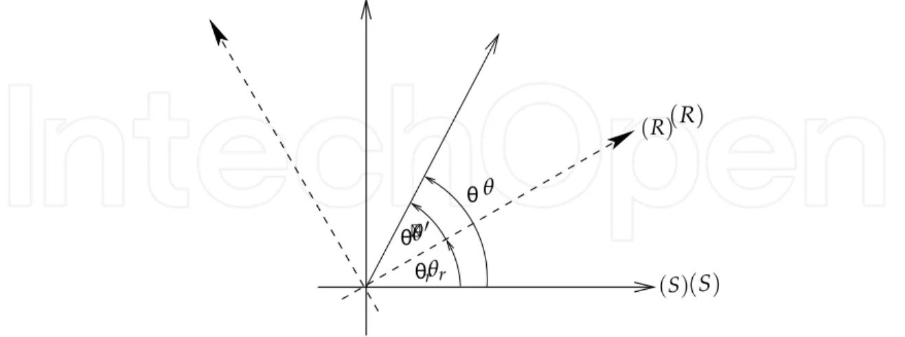
The oscillations of the mechanical rotor positionθr act on the rotor MMF. In a healthy state without faults, the fundamental rotor MMF in the rotor reference frame(R)is a wave withp pole pairs and frequencys fs, given by:

Fr(R)(θ′,t) =Frcospθ′−sωst (4) where θ′ _{is the mechanical angle in the rotor reference frame (R) and s is the motor slip.} Higher order space and time harmonics are neglected.

r _(S) (R) θ θ′ θr (S) (R)

Fig. 1. Stator (S) and rotor (R) reference frame

Figure 1 illustrates the transformation between the rotor and stator reference frame, defined byθ=θ′_{+θr . Using (3), this leads to:}

θ′=θ−ωr0t− Γc

Thus, the rotor MMF given in (4) can be transformed to the stationary stator reference frame using (5) and the relationωr0=ωs(1−s)/p:

Fr(θ,t) =Frcos(pθ−ωst−βcos(ωct)) (6)

with:

β=p Γc Jωc2

(7) Equation (6) clearly shows that the load torque oscillations at frequency fc lead to a phase

modulation of the rotor MMF in the stator reference frame. This phase modulation is char-acterized by the introduction of the term βcos(ωct) in the phase of the MMF wave. The

parameterβ is generally called the modulation index. For physically reasonable values J, Γ_c

andωc, the approximationβ≪1 holds in most cases.

The fault has no direct effect on the stator MMF and so it is considered to have the following form:

Fs(θ,t) =Fscospθ−ωst−ϕs (8)

ϕs is the initial phase difference between rotor and stator MMF. As in the case of the rotor

MMF, only the fundamental space and time harmonic is taken into account; higher order space and time harmonics are neglected.

2.1.2 Effect on Flux Density and Stator Current

The airgap flux density B(θ,t) is the product of total MMF and airgap permeance Λ_{. The}

airgap permeance is supposed to be constant because slotting effects and eccentricity are not taken into account for the sake of clarity and simplicity.

B(θ,t) = [Fs(θ,t) +Fr(θ,t)]Λ

=Bscospθ−ωst−ϕs

+Brcospθ−ωst−βcos(ωct)

(9)

The phase modulation of the flux density B(θ,t)exists for the flux Φ_{(t) itself, as}Φ_(t)is

ob-tained by simple integration of B(θ,t) with respect to the winding structure. The winding structure has only an influence on the amplitudes of the flux harmonic components, not on their frequencies. Therefore,Φ_{(t)in an arbitrary phase can be expressed in a general form:}

Φ_{(t) =}Φ_scos

ωst+ϕs+Φrcosωst+βcos(ωct) (10)

The relation between the flux and the stator current in a considered phase is given by the stator voltage equation:

V(t) =RsI(t) + d

Φ_(t)

dt (11)

WithV(t)imposed by the voltage source, the resulting stator current will be in a linear relation to the time derivative of the phase fluxΦ_{(t) and will have an equivalent frequency content.}

Differentiating (10) leads to: d

dtΦ(t) =−ωsΦssin

ωst+ϕs

−ωsΦrsinωst+βcos(ωct)

+ωcβΦrsinωst+βcos(ωct)sin(ωct)

The amplitude of the last term is smaller than that of the other terms becauseβ≪_{1. Thus, the}

last term in (12) will be neglected in the following.

As a consequence, the stator current in an arbitrary phase can be expressed in a general form:

Ito(t) =ist(t) +irt(t)

=Istsin(ωst+ϕs) +Irtsinωst+βcos(ωct)

(13) Therefore the stator current I(t)can be considered as the sum of two components. The term

ist(t)results from the stator MMF and it is not modulated. The termirt(t), which is a direct consequence of the rotor MMF shows the phase modulation due to the considered load torque oscillations. The healthy case is obtained forβ=0.

In this study, the time harmonics of rotor MMF and the non-uniform airgap permeance have not been considered. However, the harmonics of supply frequency fs and the rotor slot har-monics will theoretically show the same phase modulation as the fundamental component.

2.2 Airgap Eccentricity

Airgap eccentricity leads to an airgap length that is no longer constant with respect to the stator circumference angleθand/or time. In general, three types of airgap eccentricity can be distinguished (see Fig. 2):

Static eccentricity: The rotor geometrical and rotational centers are identical, but different from the stator center. The point of minimal airgap length is stationary with respect to the stator.

Dynamic eccentricity: The rotor geometrical center differs from the rotational center. The rotational center is identical with the stator geometrical center. The point of minimal airgap length is moving with respect to the stator.

Mixed eccentricity: The two effects are combined. The rotor geometrical and rotational cen-ter as well as the stator geometrical cencen-ter are different.

In the following theoretical development, static and dynamic eccentricity will be considered.

Rotor

Stator

(a) Static ecce ntricity (b) Dynamic ecce ntricity (c) Mixed ecce ntricity

Fig. 2. Schematic representation of static, dynamic and mixed eccentricity. ×denotes the rotor

geometrical center,∗the rotor rotational center

The airgap length g(θ,t) can be approximated for a small airgap and low levels of static or dynamic eccentricity by the following expression (Dorrell et al. (1997)):

gse(θ,t)≈g₀(1−_δscos(_θ)) gde(θ,t)≈g0(1−δdcos(θ−ωrt))

where δs, δd denote the relative degrees of static or dynamic eccentricity and g0 the mean

airgap length without eccentricity. Note that static eccentricity can be considered as a special case of dynamic eccentricity since gse(θ,t)corresponds to gde(θ,t)withωr =0, i.e. the point of minimum airgap length is stationary. Since dynamic eccentricity is more general, it will mainly be considered in the following.

The airgap permeance Λ_{(θ,t) is obtained as the inverse of g(θ,t) multiplied by the} perme-ability of free spaceµ0. Following a classical approach, the permeance is written as a Fourier

series (Cameron & Thomson (1986)): Λ_{de(θ,t) =}Λ₀₊

∞

∑

Λ_i

ecccos(ieccθ−ieccωrt) (15) whereΛ_{0=µ0/g0is the permeance without eccentricity. The higher order coefficients of the} Fourier series can be written as (Cameron & Thomson (1986)):

Λ_i ecc = 2µ0(1− √ 1−δ2)iecc g0δi_decc √ 1−δ2 (16)

Dorrell has shown in (Dorrell (1996)) that the coefficients with iecc ≥2 are rather small for δd<40%. For the sake of simplicity, they are neglected in the following considerations. The airgap flux density is the product of permeance with the magnetomotive force (MMF). The total fundamental MMF wave can be written as:

Ftot(θ,t) =F1cos(pθ−ωst−ϕt) (17)

withϕtthe initial phase. Hence, the flux density in presence of dynamic eccentricity is:

B_de(θ,t)≈B11+2 Λ₁ Λ₀cos(θ−ωrt) cos(pθ−ωst−ϕt) (18) withB1=Λ0F1

The fraction 2Λ_1/Λ_{0equals approximatelyδd for small levels of eccentricity. The airgap flux} density can therefore be written as:

B_de(θ,t) =B₁

1+δdcos(θ−ωrt)

cos(pθ−ωst₋ϕt) (19) This equation shows the fundamental effect of dynamic eccentricity on the airgap magnetic flux density : the modified airgap permeance causes an amplitude modulation of the fun-damental flux density wave with respect to time and space. The AM modulation index is approximately the degree of dynamic eccentricityδ.

In case of static eccentricity, the fundamental flux density expresses as:

Bse(θ,t) =B11+δscos(θ)cos(pθ−ωst−ϕt) (20)

which shows that static eccentricity leads only to flux density AM with respect to space. Consequently, the amplitude modulation can also be found on the stator current I(t) (see section 2.1.2) that is expressed as follows in case of dynamic eccentricity:

Ide(t) =I11+αcos(ωrt)cos(ωst−ϕi) (21) In this expression, I1 denotes the amplitude of the stator current fundamental component,

α the AM modulation index which is proportional to the degree of dynamic eccentricityδd. Static eccentricity does not lead to frequencies different fromωs since the corresponding ad-ditional flux density waves are also at the supply pulsation ωs. It can be concluded that theoretically, pure static eccentricity cannot be detected by stator current analysis.

3. Signal processing tools for fault detection and diagnosis

Theprevious section has shown that load torque oscillations cause a phase modulation on one stator current component according to (13). On the other hand, dynamic airgap eccentricity leads to amplitude modulation of the stator current (see (21)). In this section, signal processing methods for detection of both modulation types in the stator current will be presented and discussed.

In order to simplify calculations, all signals will be considered in their complex form, the so-called analytical signal (Boashash (2003)) (Flandrin (1999)). The analytical signalz(t)is related to the real signalx(t)via the Hilbert Transform H{.}:

z(t) =x(t) +jH{x(t)} (22)

The analytical signal contains the same information as the real signal but its Fourier transform is zero at negative frequencies.

3.1 Power Spectral Density 3.1.1 Definition

The classical method for signal analysis in the frequency domain is the estimation of the Power Spectral Density (PSD) based on the discrete Fourier transform of the signal x[n]. The PSD indicates the distribution of signal energy with respect to the frequency. The common estima-tion method for the PSD is the periodogramPxx(f)(Kay (1988)), defined as the square of the N-point Fourier transform divided byN:

Pxx(f) = 1 N N−1

∑

The PSD represents the basic signal analysis tool for stationary signals i.e. it can be used in case of a constant or quasi-constant supply frequency during the observation interval.

The absolute value of the Fourier transform |I(f)|of the stator current PM signal (13) is ob-tained as follows (see Blödt, Chabert, Regnier & Faucher (2006) for details):

|Ito(f)|= (Ist+IrtJ0(β)) δ(f − fs) +Irt +∞

∑

where Jn denotes the n-th order Bessel function of the first kind andδ(f)is the Dirac delta function. For small modulation indexβ, the Bessel functions of ordern≥2 are very small and may be neglected (the so-called narrowband approximation). It becomes clear through this expression that the fault leads to sideband components of the fundamental at fs±n fc. When the modulation index β is small, only the first order sidebands at fs± fc will be visible and their amplitudes will be approximately J₁(β)Irt≈0.5βIrt.

The Fourier transform magnitude of the AM stator current signal according to (21) is:

|Ide(f)|=I1δ(f −fs) + 1

2αI1δ(f −(fs± fc)) (25) The amplitude modulation leads to two sideband components at fs±fcwith equal amplitude αI₁/2. Therefore, the spectral signature of the AM and PM signal is identical if the modulation

frequency is equal and the PM modulation index is small. This can be the case when e.g. load unbalance and dynamic rotor eccentricity are considered as faults.

It can be concluded that the PSD is a simple analysis tool for stationary drive conditions. It is not suitable for analysis when the drive speed is varying. Another drawback is that PM and AM cannot be clearly distinguished.

3.2 Instantaneous Frequency 3.2.1 Definition

For a complex monocomponent signal z(t) =a(t)ejϕ(t), the instantaneous frequency fi(t) is defined by (Boashash (2003)):

f_i(t) = 1 2π

d

dtϕ(t) (26)

where ϕ(t)is the instantaneous phase anda(t)the instantaneous amplitude of the analytical signalz(t).

3.2.2 Application

The instantaneous frequency (IF) of a monocomponent phase modulated signal can be calcu-lated using the definition (26). For the phase moducalcu-lated stator current componentirt(t)(see second term of equation (13)), it can be expressed as:

fi,irt(t) = fs− fcβsin(ωct) (27)

The fault has therefore a direct effect on the IF of the stator current componentirt(t). In the healthy case, its IF is constant; in the faulty case, a time varying component with frequency fc appears.

If the complex multicomponent PM signal according to (13) is considered, the calculation of its IF leads to the following expression:

fi,I(t) = fs− fcβsin(ωct) 1 1+a(t) (28) with a(t) = I 2 st+IstIrtcos(βcos(ωct)−ϕs) I_rt2 +IstIrtcos(βcos(ωct)−ϕs) (29) Using reasonable approximations, it can be shown that 1/(1+a(t))is composed of a constant component with only small oscillations. Hence, the IF of (13) may be approximated by:

fi,I(t)≈ fs−C fcβsin(ωct) (30) whereCis a constant,C<1. Numerical evaluations confirm this approximation. It can there-fore be concluded, that the multicomponent PM signal IF corresponding to the stator current also shows fault-related oscillations at fc which may be used for detection.

The IF of an AM stator current signal according to (21) is simply a constant at frequency fs. In contrast to the PM stator current signal, no time-variable component is present. The AM modulation index α is not reflected in the IF. Consequently, the stator current IF cannot be used for amplitude modulation detection i.e. airgap eccentricity related faults.

3.3 Wigner Distribution

TheWigner Distribution (WD) belongs to the class of time-frequency signal analysis tools. It

provides a signal representation with respect to time and frequency which can be interpreted as a distribution of the signal energy.

3.3.1 Definition

The WD is defined as follows (Flandrin (1999)):

Wx(t,f) = +∞ −∞ x t+τ 2 x∗t−τ 2 e−j2πfτdτ (31) This formula can be seen as the Fourier transform of a kernelKx(τ,t)with respect to the delay

variableτ. The kernel is similar to an autocorrelation function.

An interesting property of the WD is its perfect concentration on the instantaneous frequency in the case of a linear frequency modulation. However, other types of modulations (e.g. in our case sinusoidal phase modulations) produce so-called inner interference terms in the dis-tribution (Mecklenbräuker & Hlawatsch (1997)). Note that the interferences may however be used for detection purposes as it will be shown in the following.

Another important drawback of the distribution is its non-linearity due to the quadratic na-ture. When the sum of two signals is considered, so-called outer interference terms appear in the distribution at time instants or frequencies where there should not be any signal energy (Mecklenbräuker & Hlawatsch (1997)). The interference terms can be reduced by using e.g. the Pseudo Wigner Distribution which includes an additional smoothing window (see section 3.4).

3.3.2 Application

The stator current in the presence of load torque oscillations can be considered as the sum of a pure frequency and a phase modulated signal (see (13)). The detailed calculations of the stator current WD can be found in (Blödt, Chabert, Regnier & Faucher (2006)). The following

approximate expression is obtained for smallβ:

W_ipm(t,f)≈I_rt2 +I_st2δ(f −fs) −I_rt2βsin(ωct)δ(f− fs− fc 2) +I_rt2βsin(ωct)δ(f− fs+ fc 2) (32)

The WD of the PM stator current is therefore a central frequency at fs with sidebands at fs±

fc/2. These components have time-varying amplitudes at frequency fc. It is important to note

that the lower sideband has the opposed sign to the upper sideband for a given point in time i.e. a phase shift ofπexists theoretically between the two sidebands.

The WD of the AM signal according to (21) is calculated in details in (Blödt, Regnier & Faucher

(2006)). The following approximate expression is obtained for small modulation indicesα:

W_iam(t,f)≈I₁2δ(f − fs) +αcos(ωrt)I12δ f − fs± fr 2 (33)

The AM signature on the WD is therefore sidebands at fs± fr/2. The sidebands oscillate at

similar to the PM signal but with the important difference that the upper and lower sideband oscillations have the same amplitudes for a given point in time i.e. they are in phase.

3.4 Illustration with Synthesized Signals

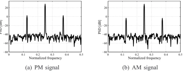
In order to validate the preceding theoretical considerations, the periodogram and WD of AM and PM signals are calculated numerically with synthesized signals. The signals are dis-crete versions of the continuous time signals in (13) and (21) with the following parameters: Ist =Irt =√2/2, I1=

√

2,α=β=0.1, ϕs =−π/8, fs =0.25 and fc = fr =0.125 normalized frequency. These parameters are coherent with a realistic application, apart from the strong modulation indices which are used for demonstration purposes. White zero-mean Gaussian noise is added with a signal to noise ration of 50 dB. The signal length isN=512 samples. First, the periodogram of both signals is calculated (see Fig. 3). Both spectra show the funda-mental component with sidebands at fs± fr. The higher order sidebands of the PM signal are buried in the noise floor so that both spectral signatures are identical.

Fig. 3. Power spectral density of synthesized PM and AM signals.

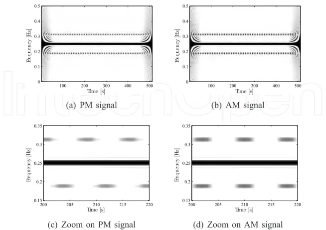
The WD is often replaced in practical applications with the Pseudo Wigner Distribution (PWD). The PWD is a smoothed and windowed version of the WD, defined as follows: (Flan-drin (1999)): PWx(t,f) = +∞ −∞ p(τ)x t+ τ 2 x∗t₋ τ 2 e−j2πfτdτ (34) where p(τ) is the smoothing window. In the following, a Hanning window of length N/4 is used. The time-frequency distributions are calculated using the MatlabR _{Time-Frequency} Toolbox (Auger et al. (1995/1996)). The PWD of the PM and AM stator current signals is dis-played in Fig. 4. A constant frequency at fs =0.25 is visible in each case. Sidebands resulting

from modulation appear at fs ± fr/2 in both cases. The zoom on the interference structure shows that the sidebands are oscillating at fr. According to the theory, the sidebands are phase-shifted by approximately π in the PM case whereas they are in phase with the AM signal.

For illustrating the stator current IF analysis, a simulated transient stator current signal is used. The supply frequency fs(t)varies from 0.05 to 0.25 normalized frequency. The

Time [s] Fr eq u en cy [H z] Time [s] Fr eq u en cy [H z] Time [s] Fr eq u en cy [H z] Time [s] Fr eq u en cy [H z]

Fig. 4. Pseudo Wigner Distribution of synthesized PM and AM signals with zoom on interfer-ence structure.

current signal is shown in Fig. 5. The linear evolution of the supply frequency is clearly visi-ble apart from border effects. With the PM signal, oscillations at varying fault frequency fc(t) can be recognized. In case of the AM signal, no oscillations are present. Further IF and PWD analysis with automatic extraction of fault indicators is described in (Blödt, Bonacci, Regnier, Chabert & Faucher (2008)).

Time [s] In s ta n ta n e o u s Fr e q u e n cy [H z] (a) PM signal Time [s] In s ta n ta n e o u s Fr e q u e n cy [H z] (b) AM signal Fig. 5. Instantaneous frequency of simulated transient PM and AM signals.

3.5 Summary

Several signal processing methods suitable for the detection of mechanical faults by stator current analysis have been presented. Classical spectral analysis based on the PSD can give a first indication of a possible fault by an increase of sidebands at fs ± fr. This method can

only be applied in case of stationary signals without important variations of the supply fre-quency. The IF can be used to detect phase modulations since they lead to a time-varying IF. A global time-frequency signal analysis is possible using the WD or PWD where a characteristic interference structure appears in presence of the phase or amplitude modulations. The three methods have been illustrated with simulated signals.

4. Detection of dynamic airgap eccentricity and load torque oscillations under lab-oratory conditions

4.1 Experimental Setup

Laboratory tests have been performed on an experimental setup (see Fig.6) with a three phase, 400 V, 50 Hz, 5.5 kW Leroy Somer induction motor (motor A). The motor has p=2 pole pairs and its nominal torqueΓ_{n is about 36 Nm. The machine is supplied by a standard industrial}

inverter operating in open-loop condition with a constant voltage to frequency ratio. The switching frequency is 3 kHz.

The load is a DC motor with separate, constant excitation connected to a resistor through a DC/DC buck converter. A standard PI controller regulates the DC motor armature current. Thus, using an appropriate current reference signal, a constant torque with a small additional oscillating component can be introduced. The sinusoidal oscillation is provided through a voltage controlled oscillator (VCO) linked to a speed sensor.

Since the produced load torque oscillations are not a realistic fault, load unbalance is also examined. Thereto, a mass is fixed on a disc mounted on the shaft. The torque oscillation produced by such a load unbalance is sinusoidal at shaft rotational frequency. With the cho-sen mass and distance, the torque oscillation amplitude isΓ_{c =0.04 Nm. If the motor}

bear-ings are healthy, the additional centrifugal forces created by the mass will not lead to airgap eccentricity.

A second induction motor with identical parameters has been modified to introduce dynamic airgap eccentricity (motor B). Therefore, the bearings have been replaced with bearings having a larger inner diameter. Then, eccentrical fitting sleeves have been inserted between the shaft and the inner race. The obtained degree of dynamic eccentricity is approximately 40%. Measured quantities in the experimental setup include the stator voltages and currents, torque and shaft speed. The signals are simultaneously acquired through a 24 bit data acquisition board at 25 kHz sampling frequency. Further signal processing is done off-line with MatlabR _.

4.2 Stator Current Spectrum Analysis

For illustration purposes, the stator current spectral signatures of a machine with dynamic eccentricity (motor B) are compared to an operation with load torque oscillations at frequency

fc = fr (motor A). In Fig. 7 the current spectrum of a motor with 40% dynamic eccentricity is

compared to an operation with load torque oscillations of amplitude Γ_{c=0.14 Nm. This}

cor-responds to only 0.4% of the nominal torque. The healthy motor spectrum is also displayed and the average load is 10% of nominal load during this test. The stator current spectra show identical fault signatures around the fundamental frequency i.e. an increasing amplitude of the peaks at fs±fr≈25 Hz and 75 Hz. This behavior is identical under different load

Fig.6. Scheme of experimental setup

Fig. 7. Comparison of experimental motor stator current spectra: 40 % eccentricity (B) vs. healthy machine (A) and 0.14 Nm load torque oscillation (A) vs. healthy machine (A) at 10% average load.

The stator current with load unbalance is analyzed in Fig. 8. A small weight has been fixed on the disc on the shaft and the amplitude of the introduced torque oscillation isΓ_{c=0.04 Nm.}

The load unbalance as a realistic fault also leads to a rise in sideband amplitudes at fs± fr. These examples show that a monitoring strategy based on the spectral components fs ± fr can be used efficiently for detection purposes. In all three cases, these components show a considerable rise. However, this monitoring approach cannot distinguish between dynamic eccentricity and load torque oscillations.

In the following, transient stator current signals are also considered. They are obtained during motor startup between standstill and nominal supply frequency. The frequency sweep rate

Frequency [Hz] P SD [d b ]

Fig. 8. PSD of stator current with load unbalanceΓ_{c = 0.04 Nm vs. healthy case}

is 10 Hz per second i.e. the startup takes 5 seconds. For the following analysis, the transient between fs=10 Hz and 48 Hz is extracted. The PSD of a healthy and faulty transient signal are displayed in Fig. 9. This example illustrates that classic spectral estimation is not appropriate for transient signal analysis. The broad peak due to the time-varying supply frequency masks all other phenomena. The faulty and healthy case cannot be distinguished.

Frequency [Hz] P SD [d b ]

Fig. 9. PSD of stator current during speed transient with load torque oscillationΓ_{c =0.22 Nm}

vs. healthy case.

4.3 Stator Current Instantaneous Frequency Analysis

In this section, instantaneous frequency analysis will be applied to the stator current signals. The original signal has been lowpass filtered and downsampled to 200 Hz in order to remove high frequency content before time-frequency analysis. Only the information in a frequency range around the fundamental is conserved.

First, a transient stator current IF is shown in Fig. 10 for the healthy case and with a load torque oscillationΓ_{c=0.5 Nm. When load torque oscillations are present, the IF oscillations increase.}

The oscillation frequency is approximately half the supply frequency which corresponds to the shaft rotational frequency fr.

Time [s] No r m a l i z e d IF

Fig.10. Example of transient stator current IF with load torque oscillation (Γ_{c =0.5 Nm) vs.}

healthy case, 25% load.

For further analysis, the IF spectrogram can be employed. The spectrogram is a time-frequency signal analysis based on sliding short time Fourier transforms. More information can be found in (Boashash (2003)) (Flandrin (1999)). The two spectrograms depicted in Fig. 11 analyze the stator current IF during a motor startup with a small oscillation ofΓ_{c =0.22 Nm}

and 10% average load. Besides the strong DC level at 0 Hz in the spectrogram, time varying components can already be noticed in the healthy case (a). They correspond to the supply frequency fs(t) and its second harmonic. Comparing the spectrogram of the healthy IF to the one with load torque oscillations (b), a fault-related component at fr(t) becomes clearly visible. More information about IF analysis can be found in (Blödt (2006)).

Time [s] Fr eq u en cy [H z] (a)healthy Time [s] Fr eq u en cy [H z] (b) c=0 .22Nm

Fig. 11. Spectrogram of transient stator current IF with load torque oscillation Γ_{c =0.22 Nm}

vs. healthy case, 10% load.

4.4 Pseudo Wigner Distribution of Stator Current

The previously considered transient signals are also analyzed with the PWD. Figure 12 shows an example of the stator current PWD during a motor startup. Comparing the healthy case to 0.22 Nm load torque oscillations, the characteristic interference signature becomes visible around the time-varying fundamental frequency. Since the fault frequency is also time vari-able, the sideband location and their oscillation frequency depend on time (Blödt et al. (2005)).

Time [s] Fr eq u en cy [H z] (a) healthy Time [s] Fr eq u en cy [H z] (b)0.22 Nm torque oscillation

Fig.12. PWD of transient stator current in healthy case and with load torque oscillation, 10% average load.

It is thereafter verified if dynamic eccentricity and load torque oscillations can be distin-guished through the stator current PWD. The stator current PWDs with dynamic eccentric-ity and with 0.14 Nm load torque oscillation are shown in Fig. 13 for 10% average load. The characteristic fault signature is visible in both cases at fs ± fr/2=37.5 Hz and 62.5 Hz. The phase shift between the upper and lower sideband seems closer to zero with eccentricity whereas with torque oscillations, it is closer to π. Nevertheless, it is difficult to determine the exact value from a visual analysis. However, the phase difference between the upper and lower sidebands can be automatically extracted from the PWD (see (Blödt, Regnier & Faucher (2006)). The result is about 125◦ with load torque oscillations and around 90◦ with dynamic eccentricity. These values differ from the theoretical ones (180◦ and 0◦ respectively) but this can be explained with load torque oscillations occurring as a consequence of dynamic eccen-tricity. A detailed discussion can be found in (Blödt, Regnier & Faucher (2006)). However, the phase shifts are sufficient to distinguish the two faults.

Fig. 13. Detail of stator current PWD with 40% dynamic eccentricity (B) and 0.14 Nm load torque oscillation (A) at small average load

5. Detection of shaft misalignment in electric winches

5.1 Problem statement

Electric winches are widely used in industrial handling systems such has cranes, overhead cranes or hoisting gears. As illustrated in Fig. 14, they are usually composed of an induction machine driving a drum through gears. Different faults can occur on such systems, leading

Fig. 14. Schematic representation of an electric winch.

to performance, reliability, and safety deterioration. A usual fault is the misalignment be-tween the induction machine and the drum, generally due to strong radial forces applied to the drum by the handled load. Theoretical and experimental studies (see for example Xu & Marangoni (1994a;b)) show that such misalignments produce mechanical phenomena, which lead to torque oscillations and dynamic airgap eccentricity in the induction machine. It has been shown in section 2 that such phenomena generate amplitude and phase modulations in the supply currents of the machine. The goal of this part is to apply to these currents some of the signal processing tools presented in section 3 in order to detect a mechanical misalign-ment in the system. Therefore, this part is organized as follows : section 5.2 describes more precisely the fault and the necessary signal processing tools, and experimental results are fi-nally presented in section 5.3.

5.2 Misalignment detection by stator current analysis 5.2.1 Shaft misalignment

Shaft misalignment is a frequent fault in rotating machinery, for which the shafts of the driving and the driven parts are not in the same centerline. The most general misalignment is a com-bination of angular misalignement (shaft centerlines do meet, but are not parallel) and offset misalignement (shaft centerlines are parallel, but do not meet). This type of fault generates reaction forces and torques in the coupling, and finally torque oscillations and dynamic airgap eccentricity in the driving machine. Moreover, these mechanical phenomena appear at even harmonics of the rotational frequencies of the driven parts (Xu & Marangoni (1994a)) (Xu & Marangoni (1994b)) (Sekhar & Prabhu (1995)) (Goodwin (1989)). For example, in the case of a misalignment of the winch shafts described in Fig. 14, torque oscillations and dynamic eccen-tricity are generated at even harmonics of the rotational frequencies of the induction machine, the gearbox and also the drum.

The theoretical model developed in sections 2.1 and 2.2 describes how mechanical phenomena are "seen" by an induction machine in its supply currents. More precisely, it has been shown that torque oscillations cause phase modulation of the stator current components (see Eq. (13)), while airgap eccentricity causes amplitude modulation (see Eq. (21)).

Therefore, in the case of a shaft misalignment in a system similar to Fig. 14, amplitude and phase modulations appear in the supply currents of the induction machine, and these modu-lations have frequencies equal to even harmonics of the rotational frequencies of the driving machine, the gearbox and the drum. Finally, the modulations generated by the drum are much more easy to detect since its rotational frequency is generally much lower than the supply and rotational frequencies of the machine fs and fr. In the following, only such low frequency modulations will be examined.

5.2.2 Shaft misalignment detection

The previous section has described that it should be possible to detect a shaft misalignment in an electric winch by analyzing its supply currents. Indeed, one only has to detect a significant increase in the amplitude and phase modulations of their fundamental component. A simple possibility is to analyze the variations of its instantaneous amplitude and instantaneous fre-quency, defined in section 3. These quantities can be easily real-time estimated as shown in (A. Reilly & Boashash (1994)), and Fig. 15 briefly describes the principle of this approach.

Fig. 15. Stator current analysis method for shaft misalignment detection.

First of all, one of the stator currents is filtered by a bandpass filter in order to obtain the funda-mental component only, without any other component. The filter used in this application has a passband only situated in the positive frequency domain around+fswith fs=45.05 Hz (see the transfer function in Fig. 15) in order to directly obtain the analytical part of the analyzed signal, as explained in (A. Reilly & Boashash (1994)). The transfer functionH(f)of this filter is therefore not hermitian (H(f)=H∗(−f)), and its impulse response is complex-valued. This particularity is not problematic concerning the real-time implementation of this filter, since its finite impulse response only needs twice as many coefficients as a classical real-valued finite impulse response filter. Finally, the output of this filter is a complex-valued monocomponent signalz(t)which represents the analytical part of the supply current fundamental component. In a second step, the modulus and the phase derivative of this complex signal lead to the in-stantaneous amplitude and frequency to estimate. Once their mean value substracted, these quantities are called amplitude modulation function (AMF) and frequency modulation func-tion (FMF). They correspond to instantaneous amplitude and frequency variafunc-tions of the cur-rent fundamental component and contain the researched modulations. Finally, power spectral densities of the AMF and FMF are estimated in order to detect and identify such modulations.

5.3 Experimental results

5.3.1 Test bench and operating conditions

A test bench has been designed by the CETIM (French CEntre Technique des Industries Mé-caniques) in order to simulate different types of faults occuring in industrial handling systems (Sieg-Zieba & Tructin (2008)). It is composed of two 22 kW Potain electric winches, and one cable winding up from one winch to the other through a pulley as shown in Fig. 16.

Fig. 16. Schematic description of the test bench.

The two winches are constituted as shown in Fig. 14, and the winch A is controlled through an inverter as a driving winch, while the winch B is only used to apply a predetermined mechanical load. The winch A is equipped with current probes in order to measure the stator currents of its induction machine. Moreover, an angular misalignment can be obtained on the same winch by inserting a shim with a slope between the motor flange and the drum bearing housing, thus creating an angle of 0.75◦_{while the tolerance of the coupling is 0.5}◦_.

During the experiments, the signals were recorded during 80 s at a sampling frequency of 25 kHz under stationary working conditions with and without misalignment. The constant mechanical load applied by the winch B was 2000 daN, and the rotational frequency reference value of the induction machine of the winch A was fr =23 Hz. These conditions resulted in

a fundamental supply frequency of fs =45.05 Hz, and a drum rotational frequency of f_{r d} =

0.29 Hz. 5.3.2 Results

Experimental results presented in this section have been obtained by applying the method de-veloped in section 5.2 to a supply current measured under the operating conditions described in the previous section. The proposed method leads to the estimation of the AMF and FMF of the stator current fundamental component, and the performance of this method is illustrated by the power spectral densities of these two functions. Low-frequency spectral contents of the AMF and FMF are respectively represented in Fig. 17 and 18. The power spectral densities obtained without any misalignment are in dashed line, while they are in solid line in case of misalignment.

As expected, amplitude and frequency modulations strongly increase in the low-frequency range when a shaft misalignment occurs, and more precisely at even harmonics of the drum rotational frequency (see arrows in Fig. 17 and 18 around 2× f_{r d} =0.58 Hz and 4× f_{r d} =

2 frd

4 frd

2 frd

2 frd

4 frd

Fig.17. Power spectral density of the AMF with (-) and without (- -) misalignment.

2 frd

4 frd

Fig. 18. Power spectral density of the FMF with (-) and without (- -) misalignment.

1.16 Hz). These results clearly show that a potential misalignment in an electric winch can be detected by analyzing its supply currents.

Furthermore, a simple and efficient misalignment detector can be derived from AMF and FMF power spectral densities. For example, the power increase of AMF and FMF in a frequency band corresponding to the expected fault can easily be estimated from these quantities by integration. In the present case, the power of these two modulation functions between 0.25 Hz and 1.25 Hz (a frequency band containing 2× f_{r d} and 4× f_{r d}) increases of about 80% (for AMF) and 120% (for FMF) when a misalignment occurs. Finally, it can be noted that such a detector can be easily real-time implemented since it is based on real-time operations only (see Fig. 15).

5.4 Conclusion

This section has shown that a shaft misalignment in an electric winch can be detected by analyzing its supply currents. Experimental results confirm that a misalignment generates additional amplitude and frequency modulations in stator currents. These phenomena can be easily detected and characterized by analyzing the spectral content of amplitude and fre-quency modulation functions of the stator current fundamental component. For example, Fig. 17 and 18 show that these additional modulations occur at even harmonics of the drum rotational frequency, i.e. in a very low-frequency range. Finally, a simple and efficient real-time detector has been proposed, based on the integration of the power spectral densities of the AMF and FMF.

6. Detection of single point bearing defects

Thefollowing section considers the detection of single point bearing defects in induction

mo-tors. Bearing faults are the most frequent faults in electric motors (41%) according to an IEEE motor reliability study for large motors above 200 HP (IEEE Motor reliability working group (1985b)), followed by stator (37%) and rotor faults (10%). Therefore, their detection is of great concern. First, some general information about bearing geometry and characteristic frequen-cies will be given. Then, a theoretical study of bearing fault effects on the stator current is presented (see Blödt, Granjon, Raison & Rostaing (2008)). Finally, experimental results illus-trate and validate the theoretical approach.

6.1 Bearing Fault Types

This paper considers rolling-element bearings with a geometry shown in Fig. 19. The bearing consists mainly of the outer and inner raceway, the balls and the cage which assures

equidis-tance between the balls. The number of balls is denotedN_b, their diameter isDband the pitch

or cage diameter is Dc. The point of contact between a ball and the raceway is characterized

by the contact angleβ.

Bearing faults can be categorized into distributed and localized defects (Tandon & Choudhury (1997)) (Stack et al. (2004b)). Distributed defects affect a whole region and are difficult to characterize by distinct frequencies. In contrast, single-point defects are localized and can be classified according to the affected element:

• outer raceway defect

• inner raceway defect

• ball defect

A single point defect could be imagined as a small hole, a pit or a missing piece of material on the corresponding element. Only these are considered in the following.

6.2 Characteristic Fault Frequencies

With each type of bearing fault, a characteristic fault frequency fc can be associated. This

frequency is equivalent to the periodicity by which an anomaly appears due to the existence of the fault. Imagining for example a hole on the outer raceway: as the rolling elements move over the defect, they are regularly in contact with the hole which produces an effect on the machine at a given frequency.

The characteristic frequencies are functions of the bearing geometry and the mechanical rotor

frequency fr. A detailed calculation of these frequencies can be found in (Li et al. (2000)). For

the three considered fault types, fc takes the following expressions:

Outer raceway: fo= Nb 2 fr 1− Db Dc cosβ (35) Inner raceway: fi= N_b 2 fr 1+ Db Dc cosβ (36) Ball: f_b= Dc D_b fr 1₋ D 2 b Dc2 cos2β (37)

It has been statistically shown in (Schiltz (1990)) that the vibration frequencies can be approx-imated for most bearings with between six and twelve balls by :

fo=0.4Nbfr (38)

fi=0.6Nbfr (39)

Fig. 19. Geometry of a rolling-element bearing.

6.3 Short Literature Survey on Bearing Fault Detection by Stator Current Analysis

Vibration measurement is traditionally used to detect bearing defects. Analytical models de-scribing the vibration response of a bearing with single point defects can be found in (Tandon & Choudhury (1997)) (MacFadden & Smith (1984)) (Wang & Kootsookos (1998)). The most of-ten quoted model studying the influence of bearing damage on the induction machine’s stator current was proposed by R. R. Schoen et al. in (Schoen et al. (1995)). The authors consider the generation of rotating eccentricities at bearing fault characteristic frequencies fc which leads to periodical changes in the machine inductances. This should produce additional frequencies

f_bfin the stator current given by:

f_bf=|fs±k fc| (40)

where fs is the electrical stator supply frequency andk=1, 2, 3, . . . .

A general review about bearing fault detection by stator current monitoring can be found in (Zhou et al. (2007)). Stack examines in (Stack et al. (2004b)) single point defects and general-ized roughness. In (Stack et al. (2004a)), the stator current is analyzed using parametric spec-trum analysis such as autoregressive modelling. Neural network techniques and the wavelet transform are used in (Eren et al. (2004)) for bearing fault detection and wavelet decomposi-tion is applied in the case of variable speed drives in (Teotrakool et al. (2006)). In (Zhou et al. (2008)) stator current noise cancellation techniques are described for bearing fault detection. In the following, a detailed theoretical study will be conducted to analyze the physical effects of bearing faults on the induction machine and the stator current. This will yield additional stator current frequencies with respect to the existing model and will give insight on the mod-ulation type.

6.4 Theoretical Study of Single Point Bearing Defects

Two physical effects are considered in the theoretical study when the single point defect comes into contact with another bearing element:

1. the introduction of a radial movement of the rotor center, 2. the apparition of load torque variations.

The method used to study the influence of the rotor displacement on the stator current is again based on the MMF (magnetomotive force) and permeance wave approach (see section 2). The following model relies on several simplifying assumptions. First, load zone effects in the bear-ing are not considered. The fault impact on the airgap length is considered by a series of Dirac generalized functions. In reality, the fault generates other pulse shapes, but this alters only the harmonic amplitudes. Since this modeling approach focusses on the frequency combinations and modulation types and not on exact amplitudes, this assumption is reasonable. The cal-culation of the airgap magnetic field does not take into account higher order space and time harmonics for the sake of simplicity. However, the calculated modulation effects affect higher harmonics in the same way as the fundamental. As before, higher order armature reactions are also neglected.

6.4.1 Airgap Length Variations

The first step in the theoretical analysis is the determination of the airgap lengthgas a function of time t and angular position θ in the stator reference frame. The radial rotor movement causes the airgap length to vary as a function of the defect, which is always considered as a hole or a point of missing material in the corresponding bearing element.

6.4.1.1 Outer Race Defect

Without loss of generality, the outer race defect can be assumed to be located at the angular positionθ=0. When there is no contact between a ball and the defect, the rotor is perfectly centered. In this case, the airgap lengthgis supposed to take the constant valueg0, neglecting rotor and stator slotting effects. On the contrary, every t=k/fo (with kinteger), the contact

between a ball and the defect leads to a small movement of the rotor center in the stator reference frame (see Fig. 20). In this case, the airgap length can be approximated by g0(1− eocosθ), where eo is the relative degree of eccentricity. In order to model the fault impact on

the airgap length as a function of time, a series of Dirac generalized functions can then be used as it is common in models for vibration analysis (MacFadden & Smith (1984)).

These considerations lead to the following expression for the airgap length: go(θ,t) =g0 1−eocos(θ) +∞

∑

equation can be interpreted as a temporary static eccentricity of the rotor, appearing only att=k/fo. The functiongo(θ,t)is represented in Fig. 21 forθ=0 as an example.

6.4.1.2 Inner Race Defect

In this case, the situation is slightly different from the outer race defect. The fault occurs at the instants t=k/f_i. As the defect is located on the inner race, the angular position of the minimal airgap length moves with respect to the stator reference frame as the rotor turns at

Fig.20. Radial rotor movement due to an outer bearing raceway defect.

Fig. 21. Airgap lengthgand permeanceΛ_{in the presence of an outer bearing raceway defect}

forθ=0.

the angular frequencyωr (see Fig. 22). Between two contacts with the defect, the defect itself

has moved by an angle described by:

∆_θi=ωr∆_t= ωr

f_i (42)

Hence, equation (41) becomes:

gi(θ,t) =g0 1−ei +∞

∑

This equation can be simplified for further calculations by extracting the cosine-term of the sum so that the series of Dirac generalized functions may be later developed into a Fourier series. One fundamental property of the Dirac generalized function is given by the following equation (Max & Lacoume (2000)):

h(k)·δ t₋ k fi =h(t f_i)·δ t₋ k fi (44) This formula becomes obvious when one considers thatδ(t−k/f_i)always equals 0, except fort=k/f_i. After combining (44), (43) and (42), the airgap length becomes:

gi(θ,t) =g0 1−eicos(θ+ωrt) +∞

∑

Fig.22.Radial rotor movement due to an inner bearing raceway defect.

6.4.1.3 Ball Defect

In presence of ball defect, the defect location moves in a similar way as the inner raceway fault. The fault causes an anomaly on the airgap length at the instantst=k/fb. The angular position

of minimal airgap length changes in function of the cage rotational frequency. Actually, the balls are all fixed in the cage which rotates at the fundamental cage frequencyωcage, given by

(Li et al. (2000)): ωcage= 1 2ωr 1₋ Db Dc cosβ (46) The angle∆_{θb by which the fault location has moved between two fault impacts becomes:}

∆_{θb =ωcage}∆t= ωcage

f_b (47)

By analogy with (45), the expression of airgap length in presence of a ball defect becomes:

g_b(θ,t) =g0 1−e_bcos θ+ωcaget + ∞

∑

6.4.1.4 Generalization

In order to simplify the following considerations, equations (41), (45) and (48) can be com-bined in a generalized expression for the airgap lengthgin presence of a bearing fault:

g(θ,t) =g0 1−ecos θ+ψ(t) + ∞

∑

ψ(t) =  



0 for an outer race defect ωrt for an inner race defect

ωcaget for a ball defect

6.4.2 Airgap Permeance

Theairgap permeanceΛ_{is proportional to the inverse of the airgap lengthgand is defined as} follows:

Λ= µ

g (51)

whereµ=µrµ0is the magnetic permeability of the airgap. In the case of a bearing fault, the permeance becomes with (49):

Λ_{(θ,t) =}Λ₀ 1 1−ecos θ+ψ(t) +∞ ∑ k=−∞ δt− _fk_c (52)

whereΛ_{0=µ/g0. The relationship between airgap lengthg(θ,t)and airgap permeance}Λ_(θ,t) is illustrated on Fig. 21 at the positionθ=0 for an outer raceway defect.

Firstly, in order to simplify this expression, the fraction 1/(1−x)is approximated for small airgap variations by the first order term of its series development:

1

1−x =1+x+x

2_+x3_{+. . . for|x|<1} ≈1+x

(53)

The condition|x|<_{1 is always satisfied because the degree of eccentricity verifies}|_e|<_{1 in}

order to avoid contact between rotor and stator.

Secondly, the series of Dirac generalized functions is expressed as a complex Fourier series development (Max & Lacoume (2000)):

+∞

∑

∑

∑

with the Fourier series coefficientsc_k= fc ∀k.

Equations (52), (53) and (54) can be combined into a simplified expression for the airgap per-meance wave: Λ_(θ,t)≈Λ₀ 1+ec0cosθ+ψ(t) +e +∞

∑

∑

6.4.3 Airgap Flux Density

Thetotal fundamental MMF waveFtotis assumed:

Ftot(θ,t) =Fcos(pθ−ωst+ϕ) (56)

Multiplication of (55) and (56) leads to the expression of the flux density distributionBtot(θ,t):

Btot(θ,t) =Ftot(θ,t)·Λ(θ,t) =FΛ_{0cos(pθ−ωst+ϕ)} + ∞

∑

whereBkare the amplitudes of the fault-related flux density waves. The notation±is used to

write all possible frequency combinations in a compact form.

Equation (57) clearly shows the influence of the rotor displacement caused by the bearing fault on the flux density. In addition to the fundamental sine wave (termB0), a multitude of

fault-related sine waves appear in the airgap. These supplementary waves have p±_{1 pole pairs} and a frequency content feccgiven by:

fecc= 1 2π ±dψ(t) dt ±kωc−ωs (58) 6.4.4 Stator Current

The additional flux density components according to (57) are equivalent to an additional mag-netic fluxΦ_{(θ,t). By considering the realization of the winding and the geometry of the}

ma-chine, the additional flux Φ_{(t) in each stator phase can be obtained. If the stator voltages}

are imposed, the time varying flux causes additional components in the motor stator current according to the stator voltage equation for the phasem:

Vm(t) =RsIm(t) + d

Φ_m(t)

dt (59)

The frequency content of the flux in each phase is supposed to be equal to the frequency content of the airgap field according to (58). Under the hypothesis of imposed stator voltages, the stator current in each phase is given by the derivative of the corresponding flux. This leads to the following expression for the stator current Im(t)withωrsupposed constant:

Im(t) = ∞

∑

Outer race defect: fecc or= fs±k fo (61)

Inner race defect: fecc ir= fs± fr±k fi (62)

Ball defect: fecc ball= fs±fcage±k fb (63)

wherek=1, 2, 3, . . . . In terms of signal processing, it can be noticed that the effect of the fault related rotor movement on the stator current is an amplitude modulation of the fundamental sine wave, due to the effect of the modified permeance on the fundamental MMF wave.

Eccentricity Torque oscillations Outer raceway fs±kfo fs±k fo

Inner raceway fs± fr±k fi fs±k fi

Ball defect fs± fcage±k fb fs±k fb

Table 1. Summary of bearing fault related frequencies in the stator current spectrum

6.4.5 Load torque oscillations

In this section, the second considered effect of a bearing fault on the machine is studied. Imag-ining for example a hole in the outer race: each time a ball passes in a hole, a mechanical re-sistance will appear when the ball tries to leave the hole. The consequence is a small increase of the load torque at each contact between the defect and another bearing element. The bear-ing fault related torque variations appear at the previously mentioned characteristic vibration frequencies fc (see section 6.2) as they are both of same origin: a contact between the defect

and another element.

The effect of load torque oscillations on the stator current has already been studied in section 2.1. The torque oscillations resulting from single point bearing defects will result in the same stator current phase modulations as described in equation (13). Note that the fault character-istic frequency fc will be take values depending on the fault type defined in section 6.2. 6.5 Summary

The results from the preceding theoretical study enlarge the existing model of the effects of bearing faults on stator current. The frequencies that can be found when the stator current PSD is analyzed, are resumed in Table 1.

6.6 Experimental Results

6.6.1 Description of Experimental Setup

The experimental tests were carried out on a test rig with a standard 1.1 kW, 2-pole pair, Y-coupled induction motor. A DC-machine was used to simulate different load levels. In order to reduce harmonic content in the supply voltage, the induction motor is directly fed by a synchronous generator (100 kVA) working as a generator. Measured quantities are the three line currents, the stator voltages, motor speed, torque and two vibration signals issued from piezoelectric accelerometers mounted on the stator core. Data are sampled at 16 kHz and processed using MatlabR _.

Two classes of faulty bearings (NSK 6205) are available. First, new bearings have been dam-aged artificially to produce defects on the outer and inner raceway. The defects consist of holes that have been drilled axially through the raceways (see Fig. 23). Secondly, bearings with realistic damage were tested, issued from industrial maintenance. The faulty bearings are mounted at the load-end of the induction machine.

The characteristic vibration frequencies take the following values at no-load operation: outer raceway frequency fo =89.6 Hz, inner raceway frequency fi=135.4 Hz, ball frequency fb =

58.8 Hz. The contact angle has been assumed to beβ=0.

6.6.2 Outer Raceway Defect

The defect on the outer raceway has already been experimentally studied in (Schoen et al. (1995)), so that it will be discussed very shortly. During the tests, the characteristic vibration

(a)outer raceway defect (b) inner raceway defect

Fig.23. Photo of bearings with single point defects

frequency and its multiples were clearly visible on the vibration spectrum of the machine. There also appeared torque oscillations at the characteristic vibration frequencies.

The current spectrum shows a characteristic component at 125 Hz which corresponds to the frequency combination|fs−2fo|(see Fig. 24). It is interesting to note, that the same frequency

combination appeared in (Bonaldi et al. (2002)) where a bearing with an outer race defect was tested experimentally.

Fig. 24. Stator current spectrum of loaded machine with outer raceway defect.

6.6.3 Inner Raceway Defect

In a first step, the vibration signal is analyzed. A logarithmic plot of the vibration spectrum with a damaged bearing in comparison with the healthy machine condition is shown in Fig. 25. The characteristic frequency of the inner raceway defect fi and its multiples (e.g. 2fi) are the components with the largest magnitude. Multiple tests with different load levels permit-ted to observe slight variations of the characteristic vibration frequency according to equation (36). Additional components due to other mechanical effects e.g. the cage rotational frequency

100 120 140 160 180 200 220 240 260 280 300 0 10 20 30 40 Frequency (Hz) Amp lit ud e PSD (d B)

inner raceway defect healthy machine

f_i