Full Vehicle State Estimation Using a Holistic Corner-based Approach

(1)

Full Vehicle State Estimation Using a

Holistic Corner-based Approach

by

Ehsan Hashemi

A thesis

presented to the University of Waterloo in fulfillment of the

thesis requirement for the degree of Doctor of Philosophy

in

Mechanical and Mechatronics Engineering

Waterloo, Ontario, Canada, 2017

c

(2)

Examining Committee MembershipThe following served on the Examining Commit-tee for this thesis. The decision of the Examining CommitCommit-tee is by majority vote.

External Examiner NAME: Goldie Nejat

Title: Associate Professor, Mechanical Engineering Supervisor(s) NAME: Amir Khajepour

Title: Professor, Mechanical Engineering Internal Member NAME: William M. Melek

Title: Professor, Mechanical Engineering Internal Member NAME: Baris Fidan

Title: Associate Professor, Mechanical Engineering Internal-external Member NAME: Dana Kulic

(3)

I hereby declare that I am the sole author of this thesis. This is a true copy of the thesis, including any required final revisions, as accepted by my examiners.

(4)

Abstract

Vehicles’ active safety systems use different sensors, vehicle states, and actuators, along with an advanced control algorithm, to assist drivers and to maintain the dynamics of a vehicle within a desired safe range in case of instability in vehicle motion. Therefore, recent developments in such vehicle stability control and autonomous driving systems have led to substantial interest in reliable road angle and vehicle states (tire forces and vehicle velocities) estimation. Advances in applications of sensor technologies, sensor fusion, and cooperative estimation in intelligent transportation systems facilitate reliable and robust estimation of vehicle states and road angles. In this direction, developing a flexible and reliable estimation structure at a reasonable cost to operate the available sensor data for the proper functioning of active safety systems in current vehicles is a preeminent objective of the car manufacturers in dealing with the technological changes in the automotive industry. This thesis presents a novel generic integrated tire force and velocity estimation system at each corner to monitor tire capacities and slip condition individually and to address road uncertainty issues in the current model-based vehicle state estimators. Tire force estimators are developed using computationally efficient nonlinear and Kalman-based observers and common measurements in production vehicles. The stability and performance of the time-varying estimators are explored and it is shown that the developed integrated structure is robust to model uncertainties including tire properties, inflation pressure, and effective rolling radius, does not need tire parameters and road friction information, and can transfer from one car to another.

The main challenges for velocity estimation are the lack of knowledge of road friction in the model-based methods and accumulated error in kinematic-based approaches. To tackle these issues, the lumped LuGre tire model is integrated with the vehicle kinematics in this research. It is shown that the proposed generic corner-based estimator reduces the number of required tire parameters significantly and does not require knowledge of the road friction. The stability and performance of the time-varying velocity estimators are studied and the sensitivity of the observers’ stability to the model parameter changes is discussed. The proposed velocity estimators are validated in simulations and road experiments with two vehicles in several maneuvers with various driveline configurations on roads with different friction conditions. The simulation and experimental results substantiate the accuracy

(5)

and robustness of the state estimators for even harsh maneuvers on surfaces with varying friction.

A corner-based lateral state estimation is also developed for conventional cars appli-cation independent of the wheel torques. This approach utilizes variable weighted axles’ estimates and high slip detection modules to deal with uncertainties associated with lon-gitudinal forces in large steering. Therefore, the output of the lateral estimator is not altered by the longitudinal force effect and its performance is not compromised. A method for road classification is also investigated utilizing the vehicle lateral response in diverse maneuvers.

Moreover, the designed estimation structure is shown to work with various driveline configurations such as front, rear, or all-wheel drive and can be easily reconfigured to operate with different vehicles and control systems’ actuator configurations such as differ-ential braking, torque vectoring, or their combinations on the front or rear axles. This research has resulted in two US pending patents on vehicle speed estimation and sensor fault diagnosis and successful transfer of these patents to industry.

(6)

Acknowledgements

First and foremost, I would like to thank my supervisor, Prof. Amir Khajepour, for his support, expertise, passion for research, encouragement, and guidance.

I also would like to acknowledge the financial support of Automotive Partnership Canada, Ontario Research Fund and General Motors. Special thanks to Dr. Bakhtiar Litkouhi, Dr. Shih-ken Chen, and Dr. Alireza Kasaiezadeh in GM Research and Devel-opment Center in Warren, MI, for their technical support and valuable inputs. I’d like to thank the technicians in the Mechatronic Vehicle Systems laboratory, Jeff Graansma, Jeremy Reddekopp, and Kevin Cochran for helping me in the road experiments.

I am deeply grateful to my friends and my family whose support is truly appreciated. Most importantly, none of this would have been possible without the love and patience of my wife, Pegah Pezeshkpour, and the many years of her support that provided the foundation for this work. My special thanks to my gorgeous son whose love has been my motivation throughout this endeavor.

My whole experience would not have been as rewarding without the help of my col-leagues, Mohammad Pirani, Milad Jalalaiyazdi, Saeid Khosravani, and Reza Zarringhalam, for their technical assistance and the stimulating discussions.

(7)

List of Tables

3.1 Parameters of the Test Vehicles for Experiments . . . 30

4.1 Force Estimators’ Error NRMS . . . 56

(11)

List of Figures

1.1 Vehicle state estimator and HVC controller . . . 3

2.1 Pure-slip LuGre tire model, normalized forces (a) longitudinal (b) lateral . 10

2.2 Combined-slip LuGre model, normalized tire forces (a) longitudinal (b) lateral 11

3.1 The proposed structure for the road angle estimation . . . 19

3.2 Height sensors and sprung mass kinematics . . . 20

3.3 Roll and pitch models with the road angles . . . 22

3.4 Experimental setup (a) the I/O and hardware layout (b) AWD test vehicle 31

3.5 Acceleration and suspension height measurements on the graded road. . . . 32

3.6 Estimation results for Case1, (a) vehicle angles (b) road grade. . . 33

3.7 Acceleration and suspension height measurements on the banked road. . . 33

3.8 Estimation results for Case2, (a) vehicle angles (b) bank angle . . . 34

3.9 Acceleration and suspension height measurements on combined grade/bank 35

3.10 Road experiments, (a) estimated vehicle angles on combined grade/bank (b) estimated road angles . . . 35

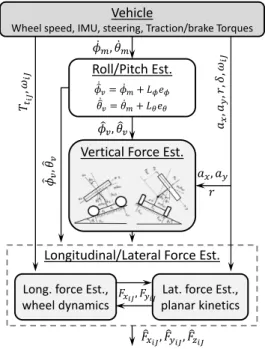
4.1 Forces and velocities in (a) planar vehicle model (b) tire coordinates. . . . 39

4.2 Corner-based force estimation structure . . . 40

(12)

4.4 (a) Electric motors (b) wheel hub sensors for force/moment measurement.. 49

4.5 Simulation results, estimated forces in CarSim (a) acceleration/brake on a road with µ= 0.3 (b) AiT on a slippery road withµ= 0.25 (c) AiT on dry asphalt. . . 51

4.6 Lane change with brake on wet, AWD vehicle (a) estimated ˆFx at rL (b)

wheel torques (c) wheel speeds (d) steering wheel angle, δsw. . . 52

4.7 DLC on snow with AWD test vehicle (a) estimated ˆFx at rL (b) rear wheel

torques (c) rear wheel speeds (d) steering wheel angle. . . 52

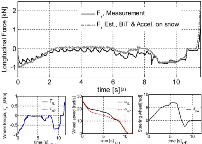
4.8 BiT and acceleration on snow for FWD case (a) estimated forces at fR with UIO (b) front wheel torques (c) rear wheel speeds (d) steering wheel angle. 53

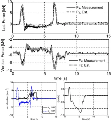
4.9 Lateral and vertical force estimation, LC for AWD on a dry surface. . . 54

4.10 Lateral and vertical force estimates, steering on ice then packed snow. . . . 55

5.1 Corner-based state estimation structure . . . 60

5.2 Time-varying observer gains for velocity estimators. . . 65

5.3 Response of the observer with time-varying gains. . . 65

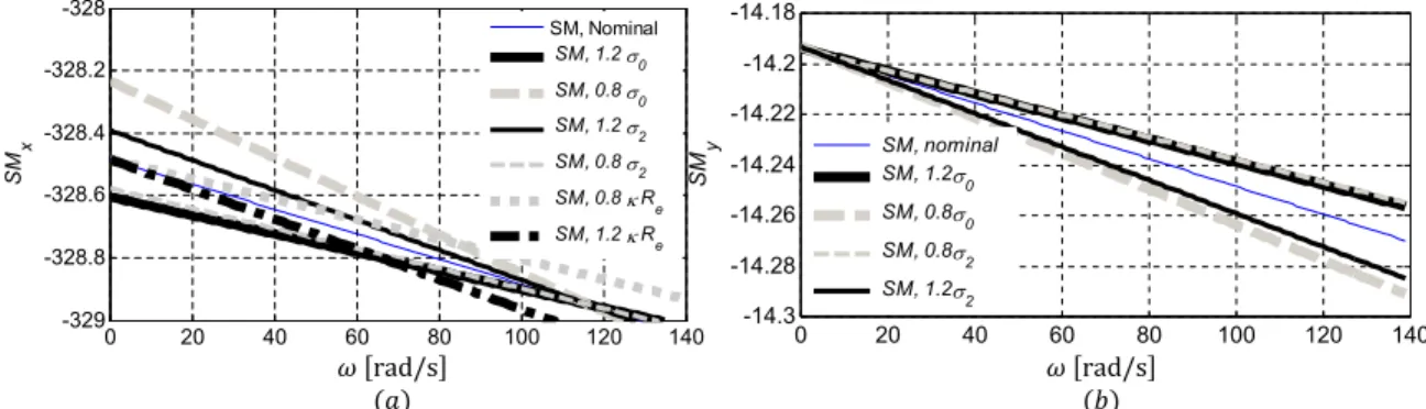
5.4 Sensitivity ofSMof the Long. and Lat. error dynamics to model parameters. 70

5.5 Sensitivity of SMof the longitudinal/lateral error dynamics to σ1q. . . 70

5.6 Sensitivity of H∞ of the Long. and Lat. error dynamics to model parameters. 71

5.7 Test1 for various road tests, experimental results . . . 75

5.8 Test2 for different driving scenarios and roads, experimental results . . . . 76

5.9 Pure-slip LuGre lateral tire model . . . 80

5.10 Normalized lateral forces, combined-slip model, on a dry road θ = 1 with longitudinal speed Vx = 20 [m/s]. . . 82

5.11 The structure of the road classifier based on the vehicle’s lateral response.. 84

5.12 The general structure of the vehicle state and road angle/condition estimation 86

(13)

5.14 Estimated Long. velocity in SS and AiT on dry/slippery roads, CarSim. . 88

5.15 Estimated velocities and wheel speeds for AWD, split-µon ice and dry. . . 89

5.16 Estimated velocities and wheel speeds for AWD, launch on a wet sealer. . . 90

5.17 Longitudinal velocity estimates for the AWD case, LC and steering on snow. 91

5.18 Velocity estimates for LC on snow/ice, for AWD configuration. . . 91

5.19 Velocity estimates for oval steering with pulsive traction on dry, RWD. . . 92

5.20 Lateral velocity estimates for RWD test vehicle, LC on combined dry/wet. 93

5.21 Lateral velocity estimates for AiT on dry asphalt, AWD configuration. . . 94

5.22 Wheel speed and estimated/measured velocities at wheel centers, AiT on dry. 94

5.23 Launch and AiT on wet sealer and wet asphalt with transition to dry for FWD (a) estimated speed (b) accelerations (c) yaw rate. . . 95

5.24 Wheel speed and estimated/measured velocities at wheel centers (Wheel C.) for (a) launch on wet sealer then dry (b) AiT on wet/dry, FWD. . . 96

5.25 Large left turn (TL) with acceleration in RWD configuration on wet/dry. . 97

5.26 Velocity estimates for AWD, BiT on snow and steering on packed snow/ice. 98

5.27 Wheel speed and estimated/measured velocities at wheel centers (Wheel C.) for (a) steering on packed snow/ice (b) BiT and acceleration on snow . . . 98

5.28 Lateral velocity estimates for AWD in an LC on packed snow and ice. . . . 99

5.29 Lateral velocity estimates for FT on dry/wet, RWD . . . 100

5.30 Lateral velocity estimates for DLC on snow, AWD . . . 101

5.31 Road classifier results and measurements for a full turn on dry asphalt, AWD103

5.32 AiT with high slip on dry asphalt, road classification for AWD . . . 104

5.33 Road classification results for AWD case in an LC on packed snow and ice 104

5.34 Full turns on dry/wet with the AWD vehicle, road classification results . . 105

5.35 AWD vehicle in full turns on dry/wet sealer . . . 106

5.36 Road classification for a mild sine steering on dry asphalt, AWD . . . 106

(14)

Chapter 1 Introduction

1.1 Motivation

Cars will become vastly safer and more intelligent through the availability of new tech-nologies in sensors, actuators, vehicle dynamic control, and autonomous systems. Studies show that utilizing safety systems such as active Vehicle Dynamics Control (VDC) and Traction Control System (TCS) plays an essential role in stability of vehicles on various road conditions with different speed (for example [1–5]), thus reducing the severity of ve-hicle accidents. In 2014 the National Highway and Traffic Safety Administration in U.S. estimated VDC (so called Electronic Stability Control, ESC) has saved close to 4000 lives during the 5-year period 2008 to 2012 and would prevent 156000 to 238000 injuries for the period in all types of crashes [6]. The United States Insurance Institute for Highway concluded that vehicles’ active safety systems reduce the likelihood of deadly single-vehicle crashes by 58% and single-vehicle rollovers by 79%. Transport Canada has also introduced the new Canada Motor Vehicle Safety Standard 126 which requires a VDC (or ESC) sys-tem on all passenger vehicles with a gross weight of 4536 kg or less, and manufactured on or after September 1st, 2011.

Examples of VDC systems already present in passenger vehicles include: anti-lock braking systems, traction control, differential braking, torque vectoring, and active steering. These systems require vehicle states (sideslip angle and speed) and individual tire states

(15)

(slip ratio, slip angle, and forces) for robust stability of a vehicle. This need is even more pronounced in a fully autonomous driving system where a human driver is completely out of the vehicle control loop.

Tire forces affect the vehicle’s capacity to perform requested maneuvers and can be measured directly with wheel hub sensors; however, such sensors cost tens of thousands of dollars, which prohibits their use in production vehicles. On the other hand, force calculation at each corner (wheel) based on a tire model requires road friction information. Thereby, even accurate slip ratio/angle information from a high precision GPS does not result in forces at each tire. Estimation of longitudinal and lateral tire forces is therefore required. In the literature, these have been estimated using Kalman-based, nonlinear, sliding mode, and unknown input observers. Force estimators are then assimilated with velocity observers to provide inputs to active safety systems of traditional and autonomous vehicles.

Information about longitudinal and lateral velocities is significant contributor in trac-tion and stability control systems. They can be measured with GPS, however, poor accu-racy and low bandwidth of available commercial GPSs, particularly for measuring velocity in the lateral direction, and loss of reception and reliability in road tunnels or in urban canyons are primary impediments to their use for active vehicle safety systems. Therefore, reliable velocity estimation that is robust to changing road and environmental conditions, and variations in model parameters have been a major focus in recent research on vehicle stability control and autonomous driving systems.

Figure1.1illustrates motivation for having vehicle states in a structure of the integrated holistic vehicle control (HVC)-Estimator.

Two major approaches have been adopted in the literature to tackle velocity estima-tion problems. One is the modified kinematic-based approach, which implements stochastic estimators or nonlinear observers using acceleration/yaw rate measurements from the In-ertial Measurement Unit (IMU). This method does not need tire model information, but instead sensor bias and noise need to be identified precisely to obtain reliable outcomes. Moreover, this approach requires a method to cope with low-excitation cases, which bring about erroneous estimations. To improve estimation results and address low excitation scenarios, kinematic-based methods could benefit from GPS measurements if reliable data is available.

(16)

, , Desired values

,

Estimated velocities at vehicle’s CG and corners , , ,

Force estimation at corners ,

Lack of sensory Meas. for tire forces, sideslip angle and slip ratio

Estimation of the longitudinal & lateral velocities & forces Vehicle HVC Controller ‐ Torque vectoring ‐ Diff. braking ‐ Active steering State Estimator

Fig. 1: State estimator with the HVC controller Meas.

Vehicle States

Figure 1.1: Vehicle state estimator and HVC controller

The other velocity estimation practice is model-based and utilizes IMU data (acceler-ation/yaw rate measurements) and corrects the estimation with tire forces using sliding mode, nonlinear, and stochastic observers. Although this approach seems promising, it requires accurate tire parameters and a good perception of road friction, especially for the tires saturation region, which is not practically feasible. Therefore, developing a holistic corner-based vehicle state estimator using conventional sensor measurement robust to the road friction changes and model uncertainties is desirable and is addressed in this research by designing observers for the consequent time-varying models.

Road grade and bank angles considerably affect the vehicle dynamics and measured accelerations, thus play a key role in the vehicle state estimation and stability. Thereby, road angle estimation is an inherent part of state of the art vehicle state estimators and is tackled in this thesis by implementing unknown input observers on vehicle pitch and roll dynamics.

1.2 Objectives

The main objective of this thesis is to develop a generic corner-based estimation of the vehicle states and road angles robust to the road friction conditions regardless of the vehicles driveline configuration (FWD, RWD, AWD). The following are detailed objectives of this thesis to provide vehicle states and road angles for VDC systems:

(17)

The first objective of this thesis is real-time estimation of the road and vehicle angles without using road friction and tire force information. Road and vehicle angles are crucial in accurate estimation of tire forces, vehicle speeds, and hence in longitudinal and lateral slip calculations. The road-body kinematics should be employed to relate the vehicle’s frame, body, and road angles and to increase the accuracy. An Unknown input observer module is introduced in this thesis which uses estimated vehicle angles and their rates for the bank/grade estimation.

The second objective of this thesis is to estimate tire forces without having road fric-tion informafric-tion for active safety systems in the newly developed Holistic Vehicle Control (HVC) paradigm. Kalman-based observers are employed on the longitudinal/lateral vehicle dynamics and wheel dynamics to estimate tire forces in real-time without any road friction data or any limiting assumption on vertical load distribution. This independent corner-based estimation structure meets the requirements of the traction and stability control systems, enhances vehicle safety, and can be transferred from one vehicle to another.

The third objective is to develop reliable real-time holistic velocity estimators at each corner robust to surface friction changes independent of the powertrain configuration in dif-ferent driving scenarios, especially for combined-slip and low-excitation maneuvers, which are arduous for the current vehicle state estimators. The newly proposed velocity estima-tor in this research combines both kinematic and dynamic-based methods and incorporates tire deflection states to form a linear parameter-varying (LPV) system in which the road friction and sensor noises are considered to be uncertainties. Road tests confirm the valid-ity of the algorithm on slippery roads as well as normal conditions. The current findings of the friction-independent velocity estimator have important implications on a joint road friction classification and state estimation scheme. A wheel torque-free lateral velocity estimator is also required for conventional vehicle applications and is an objective for the proposed estimators. Moreover, a road friction classifier, which performs in low-excitation regions as well as near-saturation and nonlinear regions, is another objective of this thesis. This road classifier can introduce new bounds on model uncertainties, which results in more accurate and less conservative observers for parameter-varying velocity estimators.

(18)

1.3 Thesis Outline

The background and literature review of road angle estimation, tire force estimation, and vehicle velocity estimation is presented in the second chapter of this thesis. The literature on vehicle state estimation is reviewed considering the fact that surface friction information is unavailable in the model-based approaches. The literature review on road condition estimation is also provided in the second chapter.

In the third chapter, a structure is provided for estimation of the road angles. The body angles are estimated using corners’ displacements measured by the suspension height sensors installed at four corners. An unknown input observer robust to acceleration noises and road uncertainties is then developed on the roll and pitch dynamics of the vehicle to estimate the road bank and grade using body angles. Knowledge of tire parameters and road friction is not required in the proposed structure. The correlation between the road angle rates and the pitch/roll rates of the vehicle are also investigated to increase the accuracy. Performance of the proposed approach in reliable estimation of the road angles is experimentally demonstrated through vehicle road tests.

In the fourth chapter, a generic corner-based force estimation method to monitor tire capacities is presented. This is entailed for more advanced vehicle stability systems in harsh maneuvers. A nonlinear and a Kalman observer is utilized for estimation of the longitudinal and lateral friction forces. The stability and performance of the time-varying estimators are explored and it is shown that the developed integrated structure is robust to model uncertainties, does not require knowledge of the road friction, and can be transferred from one car to another. Software co-simulations are utilized to test the proposed force estimation method using MATLAB/Simulink and CarSim packages. Road experiments are also conducted on different road surface conditions. The simulations and road experiments demonstrate the effectiveness of the estimation approach in diverse driving conditions.

Chapter five presents a vehicle velocity estimator by integrating the lumped LuGre tire model and the vehicle kinematics to deal with model-based and kinematic-based velocity estimation issues. It is shown that the proposed corner-based estimator does not require knowledge of the road friction, is robust to model uncertainties such as tire parameters and inflation pressure, and can be easily reconfigured to operate with different vehicles. The stability of the time-varying longitudinal and lateral velocity estimators is explored.

(19)

An integrated lateral velocity estimator is also developed that is independent of the wheel torques and utilizes wheel speed, accelerations, yaw rate, and steering angle which are com-mon in production vehicles. Moreover, a road friction classification approach is discussed and experimentally verified in low-excitation as well as nonlinear regions in this chapter. A generic joint estimation algorithm is introduced to classify the road friction condition and define tire capacities based on matching vehicle lateral responses to the expected responses on dry and slippery surfaces using pure and combined-slip friction models. The proposed methods are experimentally validated in several maneuvers with low and high levels of excitation and various driveline configurations on dry and slippery surfaces. The results exhibit promising performance of the velocity estimators and road classifier in different test conditions for both electric and conventional vehicles.

(20)

Chapter 2 Literature Review and Background

This chapter focuses on different approaches of vehicle state estimation, including kinematic-based and model-kinematic-based. Tire models and their significance on estimation methods are also provided. Finally, literature review on road angle and condition estimation is presented.

2.1 Tire Forces

Tire-road forces have played a vital role in state of the art developments in the field of vehicle state estimation and control. They are incorporated into the lateral dynamics to estimate vehicle states and analyze the vehicle stability on different roads. Tire curves are represented by three regions including linear, transient, and nonlinear defined by road fric-tion coefficient, normal forces, and cornering stiffness. The generated longitudinal/lateral forces at each tire’s patch during traction, braking, and cornering maneuvers are realized to depend on the road condition, slip ratio, slip angle, and normal forces which represent a one-to-one mapping between forces and slip values.

The most widely used static tire model, known as the Magic Formula, was proposed by Pacejka et al. [7], [8], and Uil [9], and provides a semi-experimental approach for tire force calculation. This suggested friction expression is derived heuristically from experimental tests and is generated using specific experimental data that allow independent linear and angular velocity modulation in the steady-state condition. One advantage of this model

(21)

is that it does not have differential equations in each form of partial or ordinary, making it an appropriate choice for real-time simulations. This model focuses on the steady-state response of the tires versus slip and is generated based on empirical data. The Magic Formula can be described as Y =Dsin [Ctan−1(Bφ)] +Sy with φ = (1−E)(X+Sh) +

E B

tan−1[B(X+Sh)] where Y could be longitudinal/lateral forces or the self-aligning

moment, Sh, Sy are horizontal and vertical shifts respectively, B is the stiffness factor, C

is the shape factor, D is the peak factor, E is the curvature factor, and Slip ratio/angle are the input to these equations and are denoted byX.

Steady-state assumption in the aforementioned model will not lead to precise outcomes during transient acceleration/barking maneuvers. Therefore, dynamic models seem more reliable for considering the transient phases as examined in [10–12]. Canudas-de-Wit et al. proposed a dynamic tire-road friction model, known as the LuGre, in [13–15], and introduced tire deflection as a state. Pre-sliding and hysteresis loops as well as combined friction characteristics are considered in their model [16].

Compared to other conventional approaches, e.g. Pacejka, the LuGre model utilizes relative velocities vrx = Reω−vxt and vry = −vyt rather than slip ratio λ = _max_{_Rvrx_e_ω,v_xt_}

and slip angleα = tan−1 vyt

vxt whereωis the wheel speed and Re is the tire’s effective rolling

radius. Longitudinal and lateral velocities in the tire coordinates are denoted byvxtandvyt.

The passivity of the transient LuGre makes it a bounded and stable model and prohibits the divergence of both internal tire states and consequent forces [17]. Accurate force results will be obtained by considering normal force distributions over the contact patch and multiple bristle contact points. The average lumped LuGre model [18] symbolizes the distributed force over the patch line with some simplifications of normal force distribution; representing average deflection of the bristles, the tire internal lateral state ¯zq for each

direction q∈ {x, y}in the average lumped LuGre model relates the relative lateral velocity

vrq and tire parameters as: ˙¯

zq=vrq−(κqRe|ω|+

σ0q|vrq|

θg(vrq))¯zq, (2.1a)

µq =σ0qz¯q+σ1qz˙¯q+σ2qvrq, (2.1b)

in which σ0q, σ1q, σ2q are the rubber stiffness, damping, and relative viscous damping in

(22)

pure-slip LuGre model for each direction is denoted by µq. The force distribution along

the patch line is represented by parameter κq in the average lumped model and can be

a function of time, a constant, or may be approximated by an asymmetric trapezoidal scheme. The suggested value for κq in [18] is κq = _6L7_t, where Lt is the tire patch length.

The function, g(vrq) in the pure-slip model is defined for the longitudinal and lateral

directions asg(vrq) =µcq+(µsq−µcq)e−|vrqVs| ¯ α

, in whichµcq, µsq are the normalized Coulomb friction and static friction, respectively. The Stribeck velocity Vs shows the transition between these two friction states and the tire parameter ¯α = 0.5 is assumed for this study. In the current study, identification of the LuGre tire parameters was done using the experimental curves of the Chevrolet Equinox standard tires and by utilizing an error cost function and the nonlinear least square method. The tire curve resulting from the parameters identified in the lateral direction is compared with the experimental one in Fig.A.1in the Appendix. The relative velocitiesvrx, vry at the tire coordinates of the LuGre

model represent the slip ratio λ and slip angle α in the mostly used tire models such as Burckhardt [19] and Pacejka [8] models. The level of tire and road adhesion is represented by introducing the road classification factorθwhich may vary between 0< θ ≤1 according to dry, wet, and icy conditions. Chen and Wang [20] suggested a recursive least square (RLS) estimator and an adaptive control law with a parameter projection approach for identification of this road classification parameter. Identification of this factor is also addressed in [21] by a sliding mode observer for estimation of the maximum transmissible torque and wheel slip. Steady-state normalized longitudinal and lateral pure-slip LuGre tire forces are shown in Fig.2.1for a traction maneuver on roads with different classification numbers 0.2 < θ <0.97, effective radius Re = 0.35 [m], parameters Vs = 6.2,α¯ = 0.5, tire

stiffness σ0x = 630, σ0y = 182 [1/m], rubber damping σ1x = 0.77, σ1y = 0.80 [s/m], relative

viscous damping σ2x = 0.0014, σ2y = 0.001 [s/m], load distribution factor κx = 8.3, κy =

12.9, normalized Coulomb friction µcx = 1.4, µcy = 1.2, and normalized static friction µsx = 0.8, µsy = 0.9.

Equations (2.1a), (2.1b) are developed based on the pure-slip condition, which cannot address the issue of decreasing lateral (or longitudinal) tire capacities due to the longitu-dinal (or lateral) slip. The combined-slip, i.e. direct correlation between the lateral and longitudinal slips, LuGre model is proposed by Velenis [16], in which the internal state ¯zq

(23)

(a) (b) Used for Thesis 0 20 40 60 80 0 0.2 0.4 0.6 0.8 1 Slip ratio  [%] N o rm al iz ed lo ng itudi n a l f o rc es [ -] 0 10 20 30 40 0 0.2 0.4 0.6 0.8 1

Slip angle  [deg]

No rm a liz e d la te ra l f o rc e s [ -] =0.4 =0.6 =0.8 =0.97 =0.2 =0.2 =0.4 =0.6 =0.8 =0.97

Figure 2.1: Pure-slip LuGre tire model, normalized forces (a) longitudinal (b) lateral for each direction is described as:

˙¯

zq=vrq−C0qz¯q−κRe|ω|¯zq, (2.2)

where C0j = ||Mc2vr||σ0q

g(vr)µ2cq and Mc = [µcx 0; 0 µcy]. The transient function g(vr) between

the Columb and static friction in the combined-slip tire model is introduced as:

g(vr) = ||M2 cvr|| ||Mcvr|| + _|| M2 svr|| ||Msvr|| − ||M 2 cvr|| ||Mcvr|| e−| ||vr|| Vs | 0.5 , (2.3)

whereMs= [µsx 0; 0 µsy] andvr = [vrx vry]T. The final form of the normalized friction

forceµj = Fj Fzj

of the averaged lumped LuGre model with ¯z= [¯zy z¯x]T yields [16]

µ=σ0¯z+σ1z˙¯+σ2vr, (2.4)

in which µ,z,¯ vr ∈ R2 and can be described both in longitudinal and lateral directions in

the combined or unidirectional-slip models. The longitudinal relative velocity is defined by vrx = λReω and vrx =λvxt for the traction and brake cases, respectively. In addition,

the rubber stiffness is σ0 = [σ0x 0; 0 σ0y], the rubber damping is σ1 = [σ1x 0; 0 σ1y],

and the relative viscous damping is defined by σ2 = [σ2x 0; 0 σ2y], in which σ0q, σ1q

andσ2q, are the rubber stiffness, damping, and relative viscous damping in each direction, q ∈ {x, y}. Figure 2.2 illustrates the effect of slip angle on the normalized longitudinal

(24)

forces and the effect of longitudinal slip on the normalized lateral forces. It corroborates the decreased tire capacity especially for the lateral direction in case of employing the combined-slip model which is close to real behavior of the tire.

(a) (b)

Used for Thesis

0 20 40 60 80 0 0.2 0.4 0.6 0.8 1 Slip ratio  [%] C o m b ined-sl ip nor m a lized Long. fo rc es [-] 0 10 20 30 40 0 0.2 0.4 0.6 0.8 1

Slip angle  [deg]

C o m b ined-sl ip nor m a lized L a t. fo rc e s [-] =8 =0 =17 =25 =34 =0% =25% =45% =70% =90%

Figure 2.2: Combined-slip LuGre model, normalized tire forces (a) longitudinal (b) lateral These pure and combined-slip models can be used in road-independent state estimation approaches [22,23] or incorporated in the lateral dynamics for road classification as will be described in Chapter5.

2.2 Tire Force Estimation

Tire forces can be measured at each corner with sensors mounted on the wheel hub, but their significant cost, required space, and calibration and maintenance make them com-pletely unfeasible for mass production vehicles. Provided that the tire force calculation needs road friction, even accurate slip ratio/angle information from the GPS will not en-gender forces at each corner. Hence, estimation of the longitudinal and lateral tire forces would be a remedy.

Several studies first have focused on road friction estimation and identification of tire parameters, in order to estimate longitudinal and lateral tire forces. Alvarez et al. [24] used a parameter adaptation law, a Lyapunov-based state estimator, and the dynamic

(25)

LuGre model [18] to estimate the road friction and longitudinal forces during an emergency brake condition. Employing the equivalent output error injection approach, Patel et al. proposed a second-order and third-order sliding mode observers in [25] to estimate the friction coefficient and consequently tire forces during brake on the pseudostatic LuGre [14], dynamic LuGre, and parameter-based friction [26] models. Ghandour et al. [27] developed a force and road friction estimation structure based on an iterative quadratic minimization of the error between the developed lateral force estimator and the Dugoff tire/road interaction model. Rajamani et al. [28] suggested a recursive least square for road identification and a nonlinear observer for longitudinal force estimation having wheel torques and accurate slip-ratio data from GPS. These methods rely on simultaneous road condition identification, which may impose undesirable estimation error produced by the time-varying model parameters.

Estimation of longitudinal and lateral tire forces independent from the road condition may be classified on the basis of wheel dynamics and planar kinetics into the nonlinear, sliding mode, Kalman-based, and unknown input observers. A force estimation method based on the steering torque measurement is introduced in [29,30], which requires additional measurements. Hsu et al. provided a nonlinear observer to estimate tire slip angles as well as the road friction condition in [31] with steering torque measurement.

A high gain observer with inputoutput linearization is proposed by Gao et al. [32] to estimate the lateral states. An extended Kalman filter (EKF) is employed in [33] to estimate tire forces and road friction condition simultaneously, which should handle the low excitation conditions. Baffet et al. [34] proposed a cascaded structure for estimation of the tire forces and vehicle side-slip angle with a sliding mode observer and EKF. Doumiati et al. [35] estimated tire forces with planar kinetics, EKF, and unscented Kalman filter (UKF) [36]. In their approach, longitudinal and lateral force evolution is modelled with a random walk model. They assume that tire forces and force sums on each track are associated according to the dispersion of vertical forces.

Cho et al. [37] estimated lateral tire forces using the vehicle’s planar kinetics and a random-walk Kalman filter. A Kalman-based unknown input observer (UIO) is developed by Wang et al. [38,39] for longitudinal and lateral force estimation with the wheel dy-namics, vehicle’s planar kinetics, measured wheel speeds, wheel torques, and the yaw rate. Using UKF and the wheel dynamics, Hashemi et al. [22,40] developed a longitudinal force

(26)

estimator robust to road friction changes and uncertainties in the model such as effective rolling radius, tire inflation pressure, measured wheel speed and torques. Similarly, em-ploying UKF for an antilock braking control system, Sun et al. [41] proposed a nonlinear observer robust to the road friction for the slip ratio and longitudinal force estimation. Their approach is tested during brake maneuvers on different road conditions.

2.3 Vehicle Velocity Estimation

Advanced vehicle active safety systems require dependable vehicle states, which may not be accessible by measurements, thus needing to be estimated. One major practical issues that have dominated the vehicle state estimation field is velocity estimation robust to the road friction changes to have slip ratio, slip angles, and vehicle side slip angle for the active safety systems. Longitudinal and lateral velocities make major contributions to traction and stability control systems, respectively and can be measured with GPS, but the poor accuracy of the mostly practiced conventional GPSs and the loss of reception in some areas are primary drawbacks.

Literature has adopted three major approaches for longitudinal/lateral velocity estima-tion. One is the modified kinematic-based approach, which uses acceleration and the yaw rate measurements from an inertial measurement unit (IMU) and estimates the vehicle velocities employing Kalman-based [42,43], or nonlinear [44] observers. This method does not employ a tire model, but instead the sensors bias and noise should be identified pre-cisely to have a reliable estimation. In addition, low-excitation cases that lead to erroneous estimation should be handled with this method.

To increase the accuracy of the estimated heading and position, Farrell et al. [45] used the carrier-phase differential GPS, which requires a base tower and increases the cost signif-icantly. To remove noises and address the low excitation scenarios, some kinematic-based methodologies [46,47] employs accurate GPS, which may be lost and imposes additional costs on commercial vehicles. Yoon and Peng [48] utilizes two low-cost GPS receivers for the lateral velocity estimation and compensates the low update rate issue of conventional GPS receivers by combining the IMU and GPS data using an EKF. They also proposed a vehicle state estimator by combining data of magnetometer, GPS, and IMU in [49] and

(27)

utilizing a stochastic filter integrated on the Kalman filter to reject disturbances in the magnetometer.

The other velocity estimation method integrates measured longitudinal/lateral acceler-ations and uses an observer on tire forces to correct the estimation. This approach requires a good perception of the road friction and a precise tire model. To deal with the varying tire parameters and model uncertainties, model scheduling is introduced in [50,51] using tire slips. A nonlinear observer is also provided in [52] with simultaneous bank angle esti-mation to address the unknown tire parameters. An EKF is employed for both longitudinal and lateral vehicle velocity estimation in [53,54]. EKF has been used in [55] along with the Burckhardt model [19] to estimate the vehicle states and tire model parameters; an EKF with smooth variable structure is also utilized in [56] to estimate tire slip and sideslip angles. Computational complexities of the EKF justify using a reliable approach such as UKF without any need for linearization in system dynamics. Antonov et al. employed a UKF for vehicle state estimation in [57] and provided longitudinal/lateral velocity estima-tors at each corner. They utilized wheel torques, wheel speeds, and a simplified empirical Magic formula [8] as the tire model, which requires known tire parameters and road friction. Similarly, employing UKF and knowledge of the road condition, Wielitzka et al. [58] and Sun et al. [41] proposed different methods for estimation of the lateral and longitudinal velocities using Magic formula and LuGre [13] tire models respectively.

Zhang et al. propose a sliding-mode observer in [59] to estimate velocities using wheel speed sensors, braking torque and longitudinal/lateral acceleration measurements. Their approach utilizes a sliding-mode observer for the velocity estimation and an EKF for es-timation of the Burckhardt tire model’s friction parameter. However, this method needs accurate tire parameters in presence of tire wear, inflation pressure, and road uncertain-ties. A switched nonlinear observer based on a simplified Pacejka tire model is introduced by Sun et al. [60] to provide estimates of longitudinal and lateral vehicle velocities and the tire-road friction coefficient during anti-lock braking. Their approach benefits from switching in specific cases because of unreliability of the measurements, but it relies on a predefined zero slip ratio for the longitudinal velocity measurement.

Other studies focus on the velocity estimation robust to the road condition, but im-plements additional measurements which are not common for conventional cars or require identification of tire parameters. Hsu et al. proposed a method in [29] and [31] to

(28)

esti-mate the road friction condition and sideslip angle using the steering torque sensor, which may not be applicable for all production vehicles. Nam et al. [61] presented a sideslip angle estimation method with a recursive least squares algorithm to improve stability of in-wheel-motor-driven electric vehicles, but their approach uses force measurements from the multisensing hub units, which are not available for all electric and conventional cars. A model-based vehicle lateral state estimator is developed in [62] using a a yaw rate gy-roscope, a forward-looking monocular camera, an a priori map of road superelevation and temporally previewed lane geometry. Gadola et al. investigate a Kalman-based lateral vehicle estimation on a single-track car model in [63] with the Magic formula tire model. The derivatives of the lateral forces in their approach, however, may amplify noise effects in the lateral/longitudinal state estimates.

Therefore, developing a holistic vehicle state estimator using conventional sensor mea-surement (wheel speed, steering angle, and IMU) without using road friction information is desirable and provided in this thesis.

2.4 Road Angles and Condition Estimation

Several studies investigating the vehicle stability control and state estimation have been carried out based on known road angles [57,64,65]. Direct measurement of these angles in real-time is not practical for commercial vehicles due to costs. Therefore, recent develop-ment in vehicle’s active safety systems have underlined the need for real-time estimation of the road bank and grade angles as addressed by many recent studies.

Several studies focus on estimation of road inclinations while assuming the road friction condition is known. A method for dynamic estimation of the road bank angle is discussed in [66], in which the roll and lateral dynamics are used to develop the bank angle estimator. The steady-state approximation of the bank angle is used as a reference to calculate the estimation error and design the observer. This steady-state approximation is obtained using a linear vehicle model by implementing road friction information and tire characteristics. To reduce the effects of inaccuracies in transient conditions, a dynamic factor based on the understeer coefficient in high-friction scenarios is integrated with the observer. Practical problems in terms of stability control associated with estimation stability due to switching

(29)

between the steady-state and transient conditions should be investigated. A disturbance observer is developed in [67] to estimate the vehicle roll and bank angle having the tires’ cornering stiffness and the vehicle yaw angle. Zhao et al. introduced a sliding mode observer in [68] for the velocity estimation with the road angle adaptation. Their method employs a tire model that requires the road friction and tire parameters. Menhour et al. suggest an unknown input sliding-mode observer in [69] to estimate the road bank angle. Their method employs a linear bicycle handling model for the vehicle, which needs tires’ cornering stiffness and road friction information subsequently.

Alternatively, to address the road friction uncertainties, some studies identify the road friction conditions simultaneously, which may be challenging in itself because of the issues arising from lack of excitations, tire models, etc. Grip et al. suggest a nonlinear vehicle sideslip observer in [70] that incorporates time-varying gains and road friction parameters to estimate the longitudinal/lateral velocities and road angles using a tire model. Their method suggests concurrent estimation of the vehicle states, road angles, and the road condition. A time-varying observer is utilized in [71] by Grip et al. for the concurrent estimation of the road bank and the road-tire friction characteristics. They also modulate the observer gains based on a set of practical driving scenarios to improve the performance on low-friction surfaces.

Some approaches do not implement knowledge of the road friction, but do not isolate the vehicle roll/pitch dynamics from the road inclinations. A road angle estimation is proposed by Hahn et al. in [72]. The vehicle pitch/roll induced by the suspension deflection is not separated from the road grade/bank angles. Imsland et al. suggest a nonlinear observer for the bank angle estimation in [52] to accommodate various road conditions and compared their method with an extended Kalman filter from the view point of numerical complexity. An unknown input observer is also proposed in [73] to estimate the lateral states of the vehicle as well as the bank angle. In their study, the road bank angle is assumed to be constant and its time-varying characteristics have not been taken into account in the error dynamics. A proportional integral H∞ filter is proposed by Kim et al. in [74]. They

modified a bicycle model and made the estimation algorithm more robust against model and measurement uncertainties. In their model, the vehicle roll is not separated from the road bank.

(30)

in-cluded roll/pitch dynamics with additional measurements. Utilizing a tire model and steering torque measurement, Carlson et al. offer a methodology for the separation of the road angles from the induced vehicle angles in [75] to avoid vehicle rollover. Ryu et al. used two-antenna GPS receivers to estimate the road bank and compensate the corresponding roll effect on the vehicle state estimator in [76]. Roll dynamic parameters are also identi-fied in their method. Hsu and Chen in [77] provide a model-based estimation approach for the road angles. Their method combines multiple roll and pitch models and a switching observer scheme. However, knowledge of the vehicle yaw angle, which is not accessible in commercial vehicles is required in their proposed observer.

Some literature attempted to identify the road condition and estimated vehicle states simultaneously. Grip et al. suggest a nonlinear sideslip angle observer in [70,78] that incorporates time-varying gains and estimates the vehicle states as well as the surface friction using a tire model. Their method should cope with the noises and uncertainties imposed by road identification errors due to the lack of excitation. You et al. [79] intro-duces an adaptive least square approach to jointly estimate the lateral velocities and tires’ cornering stiffness (road friction terms). The road bank angle is also identified in their approach. However, lateral acceleration measurement noises have not been addressed. A sliding-mode observer is provided by Magallan et al. in [21] based on the LuGre tire model [13] to estimate the longitudinal velocity and the surface friction.

To summarize, three main challenges exist in the current studies on the road angle and condition estimation: a) unknown tire parameters and road friction conditions; b) incor-porating effects of the vehicle roll and pitch angles;c)using available sensors and available measurements. Therefore, an estimation approach which tackles these challenges will be promising. The proposed road angle estimation approach in this thesis is independent of the road friction, investigates the road-body kinematics to relate the measured angle rates and the rate of change of the road angles, and is experimentally tested in different driving scenarios. In addition, the proposed generic road classifier compares the vehicle’s lateral response with the predicted responses on various road frictions both in low-excitation and nonlinear regions and is not sensitive to tire parameters.

(31)

Chapter 3 Estimation of the Road Angles

This chapter proposes road bank and grade angle estimators independent of the road fric-tion without limiting assumpfric-tions. The proposed estimafric-tion scheme operates in different driving scenarios as verified by road test experiments. This chapter is structured as fol-lows. First, estimation of the vehicle body’s angles, observer development on the roll/pitch dynamics, and the road-vehicle kinematics are provided. Next, an unknown input observer is proposed for estimation of the road bank and grade angles. Later, the road experiments to verify the approach in various maneuvers and driving conditions are presented.

3.1 Introduction

The proposed estimation structure is depicted in Fig. 3.1. An unknown input observer is developed to estimate the road bank and grade angles. TheSprung mass kinematic model

provides vehicle body angles ¯φv,θ¯v for the unknown input estimator.

The body angles are estimated using corners’ displacements measured by the suspension height sensors installed at corners. TheRoad-body kinematics module is employed to relate the vehicle’s frame, body, and road angles. This module relates the road angle rates and the measured angles rates by the sensors attached to the vehicle body, and provides time derivatives ˙¯φv−ij,θ˙¯v−ij of the vehicle body angles. The Unknown input observer module

(32)

, ̅ , , , , Sprung mass kinematic model

Unknown input observer on roll/pitch dynamics

Road‐body kinematics ,

, ̅

Figure 3.1: The proposed structure for the road angle estimation

uses estimated vehicle angles and their rates for the road bank/grade estimation. Details for each block are presented in the following subsections.

3.2 Sprung Mass Kinematics

The sprung mass kinematics is used to estimate the vehicle’s body roll and pitch angles

φv, θv using corners’ displacementszij. These displacements are measured by the suspension

height sensors installed at corners. A schematic of the sprung mass model and the positions of the suspension height sensors are depicted in Fig. 3.2

The auxiliary coordinates (xa, ya, za) is a right-handed orthogonal axis system obtained

by rotating the Global coordinates about the zG axis by the vehicle yaw angle ψ. The

intermediate axis system (xi, yi, zi) is given by pitch rotation θ about the ya axis (from

the auxiliary coordinates) [80]. The vehicle frame coordinates (xf, yf, zf) is also a

right-handed orthogonal axis system located at the center of the frame on undeformed body. Thus, it is parallel to the plane of the road. The subscript b represents the coordinates attached to the vehicle body as can be seen from Fig. 3.2. The sensor position vectors in the frame coordinate system (xf, yf, zf) are described as follows with i∈ {f, r}(front and

(33)

Conclusions

,

Figure 3.2: Height sensors and sprung mass kinematics rear tracks):

PiL = [di T ri/2 ziL]T, PiR = [di −T ri/2 ziR]T, (3.1)

where df and dr are the longitudinal distances between the origin Of and the front and

rear axles, respectively. The front and rear track widths are denoted by T rf and T rr,

respectively. Relative position vectors ρij,mn between two corners can be obtained by:

ρij,mn =Pmn− Pij, (3.2)

The normal vector for the sprung mass plane is then expressed as the cross product of any two relative position vectors:

N =ρij,mn×ρij,pq, (3.3)

in which the subscripts ij, mn, pq ∈ {f L, f R, rL, rR} represent front-left (f L), front-right (f R), rear-left (rL), and rear-right (rR) corners. Therefore, by using any three suspension height sensor data and corner positions, the respective normal vectors can be written as N−f L = ρrL,rR×ρrR,f R, N−f R =ρf L,rL×ρrL,rR, N−rL =ρrR,f R ×ρf R,f L, and N−rR = ρf L,rL×ρf L,f Rwhere the subscript−ijrepresents a scenario in which the suspension height

provided by sensorij is not used. Subsequently, components N−ij = [N−xij N y

−ij N−zij]T

are used to estimate the vehicle angles. The roll and pitch angles ¯φv−ij,θ¯v−ij can be written

as follows with incorporation of the corresponding normal vector N−ij:

¯ φv−ij =cos −1 N y −ij ||N−ij|| , θ¯v−ij =cos −1 N x −ij ||N−ij|| . (3.4)

(34)

Four estimates for the vehicle roll angle, and four estimates for the vehicle pitch angle, can be obtained using different combinations of the suspension sensors, then a weighted average will be used as follows to have reliable estimates in case of existing outlier data due to uneven surfaces at each corner.

The four estimated vehicle’s roll and pitch angles from (3.4) (four combinations of set of three corners) are examined to check the possibility of being an outlier because of road disturbances such as bumps and uneven surfaces at each corner. Validity of the vehicle’s roll/pitch angles is checked at two stages. First, all four angles ¯φv−ij,θ¯v−ij are compared to

each other with variance checking scheme to eliminate the one with the largest deviation. Second, for each corner, the residuals of the vehicle angle rates are defined as the difference between the time derivatives of the estimated angles ˙¯φv−ij,θ˙¯v−ijat 200[Hz]and the measured

vehicle’s angle rates ˙φs,θ˙s: R_φ−˙¯

ij =|

˙

φs−φ˙¯v−ij|, R_θ−˙¯ _ij =|θ˙s−θ˙¯v−ij|. (3.5)

When there is no disturbance at each corner, all corners’ residualsR_φ−˙¯

ij, Rθ−˙¯ ij fall below

a certain thresholdTq =Tsq+Teq(|ax|+|ay|) whereq ∈ {φ, θ}. The static minimum value

for the threshold is denoted by Tsq, and Teq introduces the effect of longitudinal/lateral excitations to the threshold. Low-pass filters can also be utilized to smooth the time derivatives of the estimated angles. After isolation of the outliers by the mentioned two tests, weighted vehicle angles ¯φv−ij,θ¯v−ij from each combination of the three corner sensors

are employed in the estimation of the vehicle’s roll/pitch angles as follows [81]: ¯ φv = X ij γ−ijφ¯v−ij, θ¯v = X ij γ−ijθ¯v−ij, (3.6)

where the weight of each three sensor combination is denoted by γ−ij and is set to 0.25

(average of the calculated angles) for the case in which there is no outlier. Whenever a disturbance or an outlier is detected in the suspension height sensor measurement at a corner, three weights will be zero since the subsequent three estimated body angles by such an outlier is not reliable. For instance, when there is a disturbance at the front-right suspension height sensor, its residuals exceed the thresholds Tφ, Tθ, thus the only

non-zero weight will be γ−f R and all other three weights will be zero. When more than one

(35)

incorporates the previously estimated valid body angles. The estimated vehicle angles (3.6) are employed for the unknown input observer to estimate the road angles as will be discussed in the following subsection.

3.3 Unknown Input Observer for Road Angle

Estima-tion

This section presents a methodology to estimate the road angles using unknown input observers (UIO). The problem of constructing an observer for systems with unknown inputs (epitomizing disturbances, faults, and uncertainties) has been widely tackled in literature with realizing full and reduced-order observers [82–85] and turns out to be considerably useful in diagnosing system faults [86–88]. A general form of the UIO is utilized in this section to estimate the unknowns (terms representing the road angles) with implementation of the vehicle body angles and their rates as the outputs. Roll and pitch dynamic models in the ISO coordinates are used for the proposed UIO and graphically illustrated in Fig.3.3. The road bank and grade angles are denoted by φr and θr respectively.

݉௦݃ _݉௦݃

Figure 3.3: Roll and pitch models with the road angles

Employing vehicle kinematics, the roll and pitch dynamics can be expressed as ˙xφ = Aφxφ+Bφuφ and ˙xθ = Aθxθ+Bθuθ where the states are xφ = [φv φ˙v]T, xθ = [θv θ˙v]T

(36)

pitch dynamics yield: ˙ xφ =   0 1 −Kφ Ix+msh2rc −Cφ Ix+msh2rc  xφ+ " 0 mshrc Ix+msh2rc # uφ, (3.7) ˙ xθ =   0 1 −Kθ Iy+msh2pc −Cθ Iy+msh2pc  xθ+ " 0 mshpc Iy+msh2pc # uθ, (3.8)

in which road bank and grade angles φr, θr appear in unknown inputs uφ, uθ. In (3.7) and (3.8), the distances between the roll/pitch axes and the center of gravity are denoted by

hrc and hpc. The moments of inertia about the roll and pitch axes parallel to the frame

coordinate system are shown byIx, Iy. Roll/pitch stiffnessKφ, Kθ and dampingCφ, Cθ are

used for derivation of the roll and pitch dynamics. The unknown longitudinal and lateral inputs are denoted by:

uφ= ˙Vy+rVx+gsin( ¯φv+φr),

uθ =−V˙x+rVy +gsin(¯θv+θr), (3.9)

in whichφr and θr show the road bank and grade respectively. The vehicle’s yaw rate r is

measured by the available stock inertial measurement unit (IMU) sensor. The longitudinal and lateral velocities Vx, Vy can be measured by a GPS or can be estimated using linear,

nonlinear, or Kalman-based observers provided in literature [22,23,33,41,57,64,90,91] Therefore, systems (3.7), (3.8) can be rewritten as ˙xq =Aqxq+Bquq and yq =Cqxq+ Dquq with q ∈ {φ, θ}and the state vectorsxq ∈_R2_{, unknown input vector} _uq _∈

R, output y∈_R2_{, and system matrices} _{Aq, Bq, Cq, Dq} _{of appropriate dimensions where [}_Bq _Dq_]T _is

full column rank and . The road angles also appear as unknown parameters in roll/pitch dynamics (3.7), (3.8). An unknown input observer [84,87] is designed to estimate the road bankφr and road gradeθr (unknown inputsuq) using vehicle body’s roll/pitch angles

¯

φv,θ¯v and their rates ˙¯φv,θ˙¯v as measurements. Derivation of the vehicle roll/pitch rates are

discussed at the end of the next subsection Road-body kinematics.

To develop the observer for practical application, discretization of the systems (3.7), (3.8) is performed by the Step-Invariance method.

(37)

Remark 1. In general, discretization of the continuous-time system x˙ =Ax+Bu with the output y=Cx+Du is done by the zero-order hold (step-invariance) method [92], because of its precision and response characteristics. Input to the continuous-time system is the hold signal uk =u(tk) for a period between tk ≤ t < tk+1 with the sample time Ts. Then,

the discrete-time system has the output matrices C¯ =C,D¯ =D and state/input matrices

¯

A=eA(t)Ts_,_B¯ ₌RTs

0 e

A(t)τ_B₍_t₎_dτ

Thus, the discrete-time form of the roll and pitch dynamics yields:

xqk+1 = ¯Aqxqk+ ¯Bquqk

yqk = ¯Cqxqk + ¯Dquqk, (3.10)

The system (3.10) have anL-delay inverse if it is feasible to uniquely recover the unknown inputuqk from the initial statex0 and outputs up to time step k+Lfor a positive integer L; the least integer L which leads to L-delay inverse is the inherent delay of the system. The upper bound on the inherent delay is defined asL _, n−N ull( ¯Dq) + 1 in [93]. The

output equation from (3.10) can be accumulated for L time steps:           yq0 yq1 yq2 .. . yqL           =           ¯ Cq ¯ CqA¯q ¯ CqA¯2q .. . ¯ CqA¯Lq           x0+           ¯ Dq 0 0 · · · 0 ¯ CqB¯q D¯q 0 · · · 0 ¯ CqA¯qB¯q C¯qB¯q D¯q · · · 0 .. . ... ... . .. ... ¯ CqA¯Lq−1B¯q C¯qA¯qL−2B¯q C¯qA¯Lq−3B¯q D¯q                     uq0 uq1 uq2 .. . uqL           (3.11)

which can be expressed as:

yq0:L =OLqx0+JLquq0:L, (3.12)

whereJLq is the invertibility matrix of the system (3.10),L is required for recovery ofxq0

from the outputyq0:L, andOLq is the observability matrix for the pair ¯Aq,C¯q. Observability

and invertibility matrices are provided in the Appendix. When the start point is the sample timek, (3.12) yields yqk:k+L =OLqxk+JLquqk:k+L.

Without loss of generality, the matrix hB¯q ¯ Dq

i

is assumed to be full rank [87] (this can be enforced by a proper transformation on the unknown inputs). Thus, there exists a matrix

(38)

¯

S such that ¯ShB¯q ¯ Dq

i

=Ip. The unknown input observer for a positive arbitrary L results

in the following estimator, which provides the states ˆxφ_k,xθˆ_k as well as unknown inputs ˆ uφ_k,uθˆ_k: ˆ xqk+1 =Eqxˆqk+Fqyqk:k+L, (3.13) ˆ uqk = ¯S " ˆ xqk+1−A¯qxˆqk yq_k −Cq¯ xqˆ _k # , (3.14)

whereEqandFq are observer gain matrices obtained by pole placement as will be described

in the following. The general form of the discrete-time system (3.10) with state vector

xq ∈ Rn, output yq ∈ Rm, and unknown input vector uq ∈ Rp has the observability and

invertibility matrices OLq ∈ Rm(L+1)×n,JLq ∈ Rm(L+1)×p(L+1) and observer gain matrices Eq ∈ Rn×n, Fq ∈Rn×m(L+1) respectively. Thereby, for the discretized form of the systems

(3.7), (3.8), the observability matrix, invertibility matrix, and observer gain matrices are OLq ∈ R2(L+1)×2,JLq ∈ R2(L+1)×(L+1) and Eq ∈ R2×2, Fq ∈ R2×2(L+1) when the vehicle

body’s roll/pitch angles and their rates ˙φv,θ˙v are utilized as measurements.

The discrete-time estimation error for the pitch and roll dynamics can be expressed as follows using (3.10), (3.12), and the unknown input observer (3.13):

eqk+1 = ˆxqk+1−xqk+1

=Eqxqˆ _k+Fqyq_k_:_k₊_L−Aqxq¯ _k−Bquq¯ _k

=Eqeqk +FqJLquqk:k+L + (Eq−A¯q+FqOLq)xqk−B¯quqk (3.15)

where the smallest Lq with upper bound Lq < n−N ull( ¯Dq) + 1 should be determined

such that rank(JLq+1)−rank(JLq) = p. In order to have asymptotic stability on the error

dynamics (3.15) regardless of xqk and inputs, Eq should be stable, i.e. |λi(Eq)| < 1,∀i ∈

{1, ..n}, and Fq should simultaneously satisfy the following [87]:

FqJLq = [ ¯Bq 0...0], (3.16)

(39)

The matrixFq is obtained from Fq = MqV where V = [0 0;Ip 0] and Mq = [ ¯Mq B¯q].

The matrix ¯Mq is chosen by a pole placement such that matrix Eq = ¯Aq−B¯qW˘q−M¯qW¯q

is stable. The matrixWq= [ ¯Wq W˘q]T is defined as Wq ,VOLq in which ˘Wq has p rows.

The stability of the state estimation error dynamics (3.15), system equations (3.10) and the estimated unknown input (3.14) guarantees that ˆuqk →uqk as k → ∞

Remark 2. An unknown input observer with delayLqcan be designed for the system (3.10)

if and only if the system is strongly detectable [84]. This is equivalent to the following conditions: rank(JLq)−rank(JLq−1) = p, (3.18) rank " Aq−zIn Bq Cq Dq #! =p+n ∀z ∈_C,|z| ≥1. (3.19)

Remark 3. The systems (3.7) and (3.8) with the discretized form (3.10) and two mea-surements (roll/pitch and their rates) is strongly detectable. Thus, a UIO can be designed for this system.

The road bank angle ˆφr is obtained as follows employing the estimated unknown input

ˆ

uφ from (3.14), the roll input definition (3.9) and the vehicle’s roll angle from (3.6):

ˆ φrk = sin −1 uˆφk−V˙yk−rkVxk g − ¯ φvk. (3.20)

Similarly, the unknown input observer (3.14) is employed for estimation of the road grade ˆ

θr, which appears as an unknown input to the pitch dynamics (3.8). Given the vehicle’s

pitch angle from (3.6), the pitch input definition (3.9) and the estimated unknown input ˆ

uθ from (3.14), the road grade is estimated as:

ˆ θrk = sin −1 uˆθk+ ˙Vxk −rkVyk g − ¯ θvk. (3.21)

The two measurements: roll/pitch angles from the suspension height sensors and their rates are used for the road grade and bank angle estimation employing the unknown input

(40)

observer (3.14) and equations (3.20), (3.21). To calculate the roll/pitch angle rates, taking time derivatives of the vehicle angles (3.6) is not a proper choice since it generates oscilla-tions due to measurement noises. Filtering such noises usually imposes undesirable delays. Thus, implementing available measurements (roll/pitch rates) from the IMU seems more promising. In order to use the measured roll/pitch rates from the sensor attached to the sprung mass, transformation between the vehicle’s frame coordinate and the body coordi-nate should be investigated. The following section focuses on the road-vehicle kinematics in order to relate the measured angle rates, vehicle body motion, and the rate of change of the road bank and grade angles.

3.4 Road-Body Kinematics

Euler angles ψ, θ, φ are utilized in this section to transform from the global coordinates (xG, yG, zG) to the vehicle frame axis system shown in Fig.3.2. These angles are successive rotations aboutzG, yaandxf respectively. Using the rotation matrices, the angular velocity of the frame relative to the global axis system can be described by ˙Γf = RGf ˙Γ where

˙Γf = [ ˙φf θ˙f ψ˙f]T is the rotation rate of the frame relative to the global coordinates

defined in the vehicle frame-fixed coordinates, and ˙Γ = [ ˙φ θ˙ ψ˙]T _{represents the rate of}

Euler angles. Defining ˙Φ = [ ˙φ,0,0]T_,_{Θ = [0}_˙ _,_θ,˙ _0]T_{, and ˙}_{Ψ = [0}_,₀_,_ψ˙_]T_{, one can write the}

rotation matrixRG f as:

RG_f =Rxf,φΦ +˙ Rxf,φRya,θΘ +˙ Rxf,φRya,θRzG,ψΨ˙, (3.22)

in whichRxf,φ shows the third rotation by an angleφabout thexf axis,Rya,θ is the second

rotation by an angleθ about theyaaxis, andRzG,ψ represents the first rotation by an angle ψ about the zG axis. Substituting rotation matrices in (3.22) yields:

RG_f =     1 0 −Sθ 0 Cφ SφCθ 0 −Sφ CφCθ     (3.23)

in whichC∗= cos(∗) andS∗= sin(∗). Road angles are defined between the vehicle frame and the auxiliary axis system (xa, ya, za) [80]. Therefore, the angular velocity of the vehicle

(41)

frame relative to the auxiliary coordinates represents the rate of change of the road angles ˙Γ_r = [ ˙φr θ˙r ψ˙r]T. Transformation (Rya,θ)

T _{from the intermediate coordinates (}_x

i, yi, zi)

to the auxiliary one is used as follows to relate the road and Euler angle rates: ˙Γ_r = (Rya,θ) T_{Φ + ˙}_˙ _{Θ =}     Cθ 0 0 0 1 0 −Sθ 0 0     ˙Γ (3.24)

Substituting ˙Γ = (RG_f)−1˙Γf into (3.24) results in:

˙Γr =     Cθ SφSθ CφSθ 0 Cφ −Sφ −Sθ −SφSθtanθ −CφSθtanθ     ˙Γf =Rf_r ˙Γf, (3.25)

in which the rotation matrixR_rf represents the transformation between the road and frame angles. The third component ˙ψr can be neglected since the yaw rate of the road is not the

concern for this study. Therefore, (3.25) is reduced to: ˙Γ_r = " Cθ SφSθ CφSθ 0 Cφ −Sφ # ˙Γ_f =χf_r ˙Γf, (3.26)

where ˙Γr = [ ˙φr θ˙r]T shows the rate of the change of the road grade and bank angles.

Afterward, employing the pseudo inverse (χf r)

−1_{, one can express the frame rotation rates}

as ˙Γf = (χfr)

−1_˙Γ

r from (3.26). The pitch and roll rate sensors are mounted on the body

sprung mass which has an orthogonal axis system (xb, yb, zb). This body-fixed coordinate

system is obtained by consecutive rotations ofφv, θvaround thexf andyf axes of the vehicle

frame coordinates, respectively. The measured rotation rate signal, ˙Γs = [ ˙φs θ˙s ψ˙s]T is

affected by the rotation rates of the body-fixed coordinate ˙Γv = [ ˙φv θ˙v ψ˙v]T, and the

frame rotation rate as ˙Γs = ˙Γv +Rfb ˙Γf. Rotation matrix Rfb is from the frame-fixed axes