University of Massachusetts Amherst University of Massachusetts Amherst
ScholarWorks@UMass Amherst
ScholarWorks@UMass Amherst
Doctoral Dissertations Dissertations and Theses
November 2016
Detecting Candidate Preknowledge of Items Using A Predictive
Detecting Candidate Preknowledge of Items Using A Predictive
Checking Method
Checking Method
xi wangFollow this and additional works at: https://scholarworks.umass.edu/dissertations_2
Part of the Educational Assessment, Evaluation, and Research Commons, and the Quantitative Psychology Commons
Recommended Citation Recommended Citation
wang, xi, "Detecting Candidate Preknowledge of Items Using A Predictive Checking Method" (2016). Doctoral Dissertations. 812.
https://scholarworks.umass.edu/dissertations_2/812
This Open Access Dissertation is brought to you for free and open access by the Dissertations and Theses at ScholarWorks@UMass Amherst. It has been accepted for inclusion in Doctoral Dissertations by an authorized administrator of ScholarWorks@UMass Amherst. For more information, please contact
DETECTING CANDIDATE PREKNOWLEDGE OF ITEMS USING A PREDICTIVE CHECKING METHOD
A Dissertation Presented
by XI WANG
Submitted to the Graduate School of the
University of Massachusetts Amherst in partial fulfillment of the requirements for the degree of
DOCTOR OF PHILOSOPHY September 2016
© Copyright by Xi Wang 2016 All Rights Reserved
DETECTING CANDIDATE PREKNOWLEDGE OF ITEMS USING A PREDICTIVE CHECKING METHOD
A Dissertation Presented by
XI WANG
Approved as to style and content by:
_______________________________________ Ronald K. Hambleton, Chair
_______________________________________ Craig S. Wells, Member
_______________________________________ Anna Liu, Member
____________________________________ Joseph B. Berger, Senior Associate Dean College of Education
DEDICATION
ACKNOWLEDGMENTS
Up until this moment, I still cannot believe five years have passed since I first came to the U.S. on August 21, 2011. Many people say one’s early twenties are the best ages in one’s life. If so, I am very lucky and happy to spend my best time in the graduate school to pursue my doctoral degree. The five years’ study and life in the U.S. has been an exciting journey for me, also filled with bitter sweet moments sometimes. At the end of this journey, I would like to express the deepest gratitude to my dear professors, friends and family.
First of all, I would like to thank my advisor Prof. Ronald. Hambleton, who is also the chair of my dissertation committee. As an advisor, Prof. Hambleton has always been very supportive for what I want to do, and he has been giving me helpful advice on my academic and career development. As an internationally renowned scholar, he is not only extremely knowledgeable of psychometrics, but also highly experienced with
applying such knowledge to solve practical problems in the real world. Besides providing suggestions on solving specific problems in my study and research, he always encourages me to come up with research questions with practical significance. He is also very modest and always fully prepared for everything, which set a role model for me to never stop making things better.
I would also like to thank my other two committee members, Prof. Craig Wells and Prof. Anna Liu. Prof. Wells has also played a very important role in my academic development. I have been fortunate to have several opportunities to work with him during the past five years. He is smart, generous and has a very solid background in
pointing out new research directions, so our collaborations are always effective and productive. Without him, I will not be able to grow so fast in my academic development. My gratitude also goes to Prof. Anna Liu, who serves as the outside committee member for my dissertation. I would like to thank her for her time and suggestions on my
dissertation.
This dissertation project is funded by Educational Testing Service (ETS) through the Harold Gulliksen Psychometric Research Fellowship. It is my great honor to be a recipient of this fellowship award. I would like to thank ETS for this funding opportunity. I am more than happy to have three excellent mentors from ETS: Drs Fred Robin,
Hongwen Guo, and Neil Dorans. They have contributed significantly to the second study in this dissertation. My mentors and I had a lot of discussions on this project while I was in Princeton last summer, which was an invaluable experience for me. Although it was often hard to reach an agreement among us, it is through those discussions that we made things better and added more practical significance to this study.
My appreciation also goes to a special friend, Dr. Yang Liu, who has made significant methodological contributions to this dissertation. In fact, the idea of this dissertation project started from my conversations with Dr. Liu. Having had a solid training in both psychometric and statistical theories, he can always provide some effective suggestions whenever I got stuck on some problems. His attitude towards research - trying to provide rigorous justification to every detail – also sets a role model for me as a young scholar.
In addition to receiving academic guidance from different people, I am very lucky to also have support and love from my family and friends. REMP is a loving family, and
I am glad to be able to share my happiness and sorrow with my dearest friends Fen Fan, Joshua Marland, Hwanggyu Lim, HyunJoo Jung, Yooyoung Park, and Hongyu Diao. The time we spent together is the best time I had in graduate school. My gratitude also goes to all REMP professors as well as Peg Louraine and Emily Pichette. In addition, I appreciate the constant care and support from my ETS intern friends, Fei Chen, Huili Liu and Xin Luo, all of whom are so smart and humorous. Their words of comfort and encouragement always have the magic to cheer me up. I would also like to thank my parents and
grandparents for raising me up, and for being understanding of my dreams.
Unfortunately, my grandma was not able to see me finishing this journey, but I know I did not let her down and she would be proud of me as always.
Lastly, I would like to express my appreciation to my husband, Mengwei Li, who is also my best friend in life. Thank you for giving up other good opportunities to come here to be with me, and thank you for bringing so much happiness into my life.
Although my journey to the Ph.D. degree is almost completed, I know that learning will not come to an end as I walk out of graduate school. Instead, it has just started.
ABSTRACT
DETECTING CANDIDATE PREKNOWLEDGE OF ITEMS USING A PREDICTIVE CHECKING METHOD
SEPTEMBER 2016
XI WANG, B.S., BEIJING NORMAL UNIVERSITY
Ph.D., UNIVERSITY OF MASSACHUSETTS AMHERST Directed by: Professor Ronald K. Hambleton
In on-demand high-stakes testing programs such as GRE and TOEFL, some items are repeatedly used across test administrations to reduce the cost of developing new items constantly. Item exposure provides an opportunity for examinees to have knowledge of particular test items in advance of their administration. It poses a threat to test security and ultimately will result in invalid test scores. Therefore, many testing programs conduct quality control to monitor test compromise at individual and/or group level. A predictive checking method is proposed in this study to detect examinee preknowledge on exposed items. We consider a scenario where a test can be divided into two subsets of items: one consisting of secure items with very low exposure rates and the other consisting of possibly compromised items (i.e. unsecure items) which have been exposed for a while. An examinee’s proficiency distribution is first obtained from secure items and then the predictive distribution for the examinee’s test scores on the unsecure items is constructed. The extent of test compromise is determined by comparing an individual’s observed score on the unsecure items with the predictive distribution. To evaluate the effectiveness of this approach, three studies are conducted: the first study investigates the statistical
properties (i.e. type-I error and power) of this method under four factors through Monte Carlo simulation; the second study applies this method to two simulated test compromise situations that are likely to happen in practice, and compares this method to three other detection approaches; the third study applies this method to a real dataset to demonstrate its practice use. Findings from the simulation studies suggest that the predictive checking method is effective in detecting examinees’ preknowledge in the unsecure subset given a moderate to large test compromise rate, while maintaining its type-I error close to or lower than the nominal level. It also demonstrates similar or better performance than the other approaches under investigation. These results have implications for conducting quality control at individual examinee level in an on-demand testing program.
TABLE OF CONTENTS
ACKNOWLEDGMENTS ...v
ABSTRACT ... viii
LIST OF TABLES ... xiii
LIST OF FIGURES ...xv
CHAPTER 1. INTRODUCTION ...1
1.1 Background ...1
1.1.1 Introduction to the Problem of Test Security ...1
1.1.2 Test Security in Adaptive Tests ...3
1.2 Statement of the Problem ...7
1.3 Research Purpose ...11
1.4 Educational Significance ...12
2. LITERATURE REVIEW ...14
2.1 Overview of Person-fit Statistics ...15
2.2 Methods Specific to Detecting Item Preknowledge ...21
2.2.1 Methods not using information from secure items ...21
2.2.2 Methods using information from secure items ...26
2.3 Summary of Existing Methods ...39
3. METHODOLOGY ...41
3.1 Predictive Checking Method...41
3.1.1 Mathematical Definition and Properties ...41
3.1.2 Implementation of Predictive Checking ...44
3.1.2.1 Estimation of𝒑(𝜽|𝒚𝟏) from T1 ...45
3.1.2.1.1 Bayesian Posterior Distribution ...45
3.1.2.2 Sampling From 𝒑(𝜽|𝒚𝟏) ...49
3.1.2.3 Test Statistics ...50
3.1.2.4 Item-set Level and Item Level Detection...51
3.2 Likelihood Ratio Test ...53
3.3 Adapted KL Divergence ...55
3.4 Regression-based approach ...57
4. STUDY 1: EVALUATION OF PREDICTIVE CHECKING ...60
4.1 Study Design ...60
4.2 Data Simulation ...62
4.3 Evaluation Criteria ...63
4.4 Results ...64
4.4.1 Recovery of 𝜽 by Different Estimation Methods ...64
4.4.2 Type-I error at the item-set level ...65
4.4.3 Power at the item-set level ...66
4.4.4 Type-I Error at the item level ...68
4.4.5 Power and False Positive Rate at the item level ...69
4.5 Discussion ...72
5. STUDY 2: COMPARISON OF METHODS ...74
5.1 Background ...74
5.2 Shallow Pool Simulation...75
5.3 Key Exposure Simulation ...79
5.4 Evaluation Criteria ...83
5.5 Results in Shallow Pool Simulation ...84
5.5.1 Theta estimation error ...84
5.5.2 Detection rate at the person-level ...88
5.5.3 Detection rate at the group level ...95
5.6 Results in Key Exposure Simulation ...99
5.6.1 Person-level Detection Result ...99
5.6.2 Group-level Detection Results ...102
5.7. Discussion ...103
6. REAL DATA APPLICATION ...107
6.3 Results ...110
6.3.1 Detection rate ...110
6.3.2 Classification Consistency ...112
6.3.3 Detection Characteristics by Different Methods ...113
7. DISCUSSION AND CONCLUSIONS ...116
APPENDICES A. TABLES ...124
B. FIGURES ...134
LIST OF TABLES
Table Page
4.1: Bias and MSE from Different Estimation Methods...65
4.2: Empirical Type-I Error Using Fiducial and Jeffreys Prior ...66
4.3: Power Rate Using Fiducial and Jeffreys Prior ...68
4.4: Empirical Type-I Error at Item Level ...69
4.5: Item-Level Power and False Positive Rate ...71
5.1: True Item Parameters in Shallow Pool Situation in Study 2 ...77
5.2: Conditions in Shallow Pool Situation ...78
5.3: Simulation Conditions in Key Exposure Situation ...81
5.4: Summary of True Item Parameters in Key Exposure Generation ...82
5.5: BIAS and RMSE in Null Condition ...85
5.6: Average θ Inflation (θ − θ) in Test Compromise Conditions ...86
5.7: Powerwith True Item Parameters ...90
5.8: Power with Item Parameter Estimates from 3PLM ...91
5.9: Power with Item Parameter Estimates from 2PLM ...92
6.1: Detection Rate (EAP change) of Different Methods ...110
6.2: Classification consistency among different methods...113
A.1: True Item Parameters in Study 1 ...124
A.2: Empirical Type-I Error at Item-set Level Using Fiducial and Jeffreys Prior ...126
A.3: Empirical Type-I Error at Item-set Level Using Normal Prior...127
A.4: Power at Item-set Level Using Fiducial and Jeffreys Prior When Compromise Rate is 100%...128
A.5: Power at Item-set Level Using Fiducial and Jeffreys Prior When Compromise Rate is 60%...129
A.7: Empirical Type-I Error at Item Level ...131 A.8: Empirical Power at Item Level ...132 A.9: False Positive Rate at Item Level...133
LIST OF FIGURES
Figure Page
1.1: Example of a 1-3-3 MST design ...6
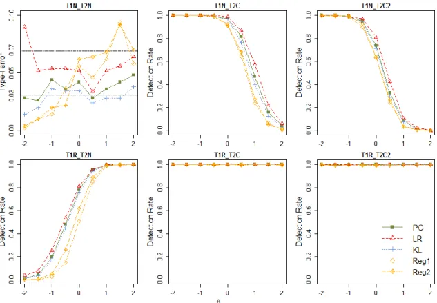
5.1: Type-I error rate at person level ...89
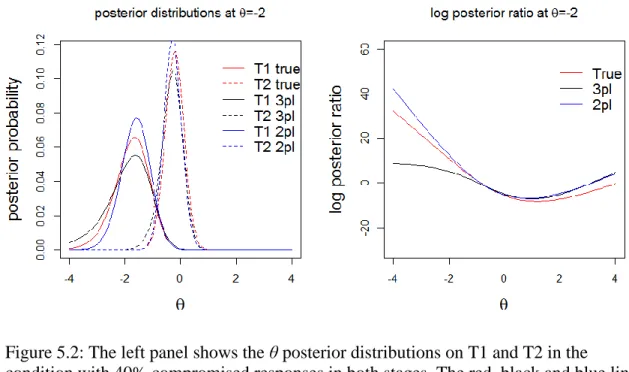
5.2: The left panel shows the θ posterior distributions on T1 and T2 in the condition with 40% compromised responses in both stages. The red, black and blue lines represent the use of true item parameters, 3PLM item parameter estimates and 2PLM item parameter estimates. The right panel shows the log posterior ratio between T1 and T2 when the three types of item parameters are used ...95
5.3: Type-I error rate of the three methods (PC=Predictive checking, KL=KL divergence, and LR=likelihood ratio) among different examinee ability groups ...96
5.4: Detection power among examinees with ability distribution of N(0,1) ...97
5.5: power among examinees with ability distribution of N(-1,1). ...98
5.6: Person-level detection rate across different conditions ...99
5.7: Distribution of standardized residuals at different θ levels. ...101
5.8: Group-level detection rate across different conditions. ...102
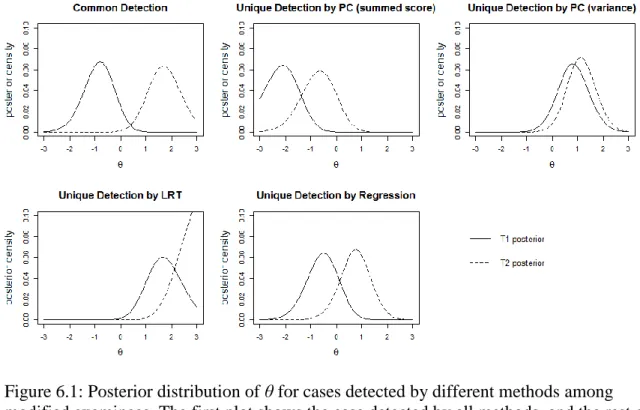
6.1: Posterior distribution of θ for cases detected by different methods among modified examinees ...114
6.2: Posterior distribution of θ for cases detected by different methods among unmodified examinees. ...115
6.3: Scatterplot of summed score (left) and EAP (right) on T1 and T2...115
B.1: Plots to check assumptions in simple linear regression in study 2. ...134
CHAPTER 1 INTRODUCTION
1.1 Background
1.1.1 Introduction to the Problem of Test Security
With the rapid advance of information technology, computer-based testing (CBT) is gradually replacing the traditional paper-and-pencil tests and becoming the mainstream in large-scale assessments in the 21st century. A number of high-stake testing programs, such as the GRE, TOEFL and SAT, have been using computer-based testing for years. Currently, the two common-core assessment consortia-the Partnership for Assessment of Readiness for College and Careers (PARCC) and SMARTER Balanced- are both
administering their annual as well as their formative tests through computers. One of the advantages that CBT offers is the “on-demand” test scheduling, which means a test is offered on a large number of time slots within a testing window, and an examinee can choose to take the test at any available time slot. Although on-demand testing brings much convenience for test takers, it becomes more difficult for the testing agency to insure test security.
Due to the large number of testing administrations in an on-demand testing, it is practically impossible to use a different test form for each test administration. The cost for item development is high. For example, in a legal case about twenty years ago, Educational Testing Service (ETS) reported that it cost them about $1000 to produce a quality test item; that figure is undoubtedly much higher today. Due to the high expenses of item development, test items are repeatedly used across different test administrations.
This provides an opportunity for examinees who take the test earlier to steal the items and then share them with future examinees. Of course, examinees are asked not to share items, and they are sometimes told that if caught, there can be seriously punished, but not all examinees follow the rules.
Examinees who take the test later can then use item preknowledge to gain score increases. Items could be stolen through some “spy” cameras that can be hidden in glasses, pens or watches (Wollack & Fremer, 2013, pp. 48), or could be stolen through earlier test takers’ memorization. The former type of item stealing could still be detected by well-trained proctors, while the later type can never be explicitly detected. The stolen items could be shared among friends, posted on the Internet, or distributed through some organized efforts. An example of organized item-theft efforts is the well-publicized 1994 ETS-Kaplan incident, where Kaplan Test Prep sent 20 of its employees to take the computerized version of the GRE to memorize as many items as possible and then reproduce the items later for some type of distribution to future examinees (Wollack & Fremer, 2013). Another example for item sharing occurred on the Graduate Management Admissions Test (GMAT). In 2008, the Graduate Management Admissions Council (GMAC) cancelled the scores of 84 students as they found those students had access to some stolen items that were posted on a website (Hechinger, 2008). GMAC also provided an example for an item posted on the website and the actual item used in the test, and showed that the memorized items had contained most of the information from the actual test item.
1.1.2 Test Security in Adaptive Tests
In this section, discussion is focused on test security problems specific to adaptive test designs, as adaptive tests have been widely applied in many high-stake testing
programs in recent years. The goal of an adaptive test is to “tailor” test items to the examinee’s ability level. The idea of using an adaptive test can be traced back to the Binet–Simon (1905) intelligence test, where the test questions were adapted to the estimate of an examinee’s mental age based on the examinee’s responses to earlier test questions. It is the use of computer-based testing that makes it possible to widely implement adaptive test in large-scale, high-stakes assessments. Adaptive tests can be further categorized into two designs according to the level of adaption: item-level adaptive tests and module-level adaptive tests. The former is often known as a
computerized adaptive test (CAT), while the latter is known as a multistage adaptive test (MST). CAT has been implemented in large-scale testing programs for decades (e.g. van der Linden & Glas, 2010). Examples include the Armed Services Vocational Aptitude Battery (ASVAB) by the U.S. Department of Defense, the nurse licensure and
certification exam (NCLEX/CAT) by the National Council of State Boards of Nursing, and the early CAT-versioned Graduate Record Examination (GRE) by ETS. Currently, CAT is being applied in SMARTER Balanced common-core assessments as well. MST, as a compromise between CAT and fixed-form test, has received increasing interest in recent years, and it is now adopted by several operational testing programs including the revised GRE General test and the Certified Public Accountant Exam.
In CAT, an examinee’s proficiency is estimated after each item is administered and the selection of the next item is based on the current proficiency estimate and on
constrains for item content and exposure. In CAT, different examinees typically are administered different items. This provides an advantage for test security as examinees taking the test later may not get exactly the same items as earlier examinees, and thus the overall item exposure rate is reduced. However, since CAT aims to select items that can provide most statistical information for an examinee’s proficiency, items with the better psychometric properties tend to be selected more often than others. This results in uneven exposure rates among different items. In addition, examinees at similar proficiency levels are likely to receive the same items, albeit in a different order. Therefore, when item-sharing is among friends, who are more likely to be of similar proficiency levels, even some items with low overall exposure rates (among the examinee population) can be compromised. Also, in organized item-theft efforts, thieves typically targeted at items with middle to high difficulty levels, so items that are more likely to be administered to high-proficiency examinees will have higher exposure rates (Stocking & Lewis, 1998).
The high exposure or conditional exposure rate of some items at a certain proficiency level leaves the item pool vulnerable to item-theft. The simulation study conducted by McLeod, Lewis, and Thissen(2003) illustrated how quickly an item pool could become compromised with an organized item-theft effort. They simulated the item memorization-sharing strategy in a 28-item CAT: a group of source examinees were simulated to take the test and memorize all the items administered to them, and then a list of memorized items was shared with beneficiary examinees who would later take the test with item preknowledge. Their results showed that when eight sources were used,
approximately 125 items out of 494 items in the pool were compromised, and the
test administration, which could result in an average score gain of 30 points out of 60 total points for low-proficiency examinees, and an average score gain of 15-20 points for medium-proficiency examinees.
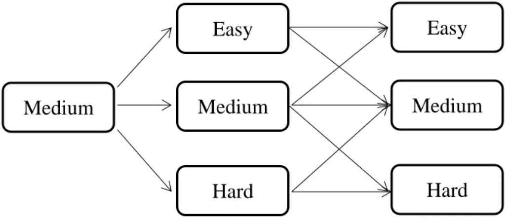
Different from CAT, an MST administers a series of sets of items adaptively to examinees (e.g. Yan , von Davier, & Lewis, 2014). Within each item set, which is called a module (also called item block or testlet), items are fixed and administered linearly to examinees (perhaps in some applications the items within a module may even be administered randomly to examinees as an additional way to enhance test security). An MST design consists of two or more stages and each stage could consist of one or more modules. At each stage, the module whose difficulty level is the most approximate to an examinee’s proficiency level is administered, subject to the routing rules implemented. Figure 1.1 below shows an example of a three-stage MST design. Stage 1 consists of a module of moderate difficulty, and all examinees receive this module. Stage 2 and 3 both consist of three modules of different difficulty levels. Based on an examinee’s
proficiency estimate from a previous stage, one of the modules in Stage 2 or 3 is administered adaptively to the examinee. In practice, numerous parallel forms are
constructed for a given module to ensure the maximum exposure of each module does not exceed a particular rate (Luecht, 2003). In this way, the item exposure rate in an MST can be controlled prior to test administration simply by specifying the number of parallel modules.
Figure 1.1: Example of a 1-3-3 MST design
Although it is easier to control item exposure rate in a MST design compared to a CAT design, the study by Wang, Zheng, and Chang (2014) suggests the use of MST may create a less secure condition than CAT in the circumstance of item-sharing and
organized item theft, if an entire MST module is repeated used. To quantify test security, they used two types of statistics: the mean and standard deviation (SD) of test overlap rate among all possible pairs of examinees, while the test overlap rate is the proportion of common items shared by any two examinees. With both analytical and simulation results, they showed that the mean test overlap is approximately the same in both CAT and MST, but the SD of test overlap rate is always larger in MST. A large SD means certain groups of examinees share a larger number of common items than others, and thus the test
overlap rate in MST tends to be more extreme in certain groups than that in CAT. A more intuitive understanding for this is that since modules are used repeated in different test administrations in MST, examinees who are administered the same module(s) will share the entire module(s) in common, while examinees who are administered different module(s) will share no items in common. Wang, Zheng, and Chang (2014) further
Medium
Easy
Medium
Hard
Easy
Medium
Hard
scenario. They found that on average, a future examinee could receive more
compromised items that are memorized by earlier test takers in MST than in CAT, which ultimately led to larger misclassification rate in MST.
1.2 Statement of the Problem
Item preknowlege forms a big threat to test security and ultimately could result in invalid test scores for many examinees. When there are a lot of compromised items or when a large number of examinees have item preknowledge, measurement accuracy and validity will be severely jeopardized and the invalid decisions or inferences made based on test scores will cause negative consequences for both the testing program and the stake-holders.
Due to the concern for the potential destructive consequences that item
preknowledge could have on test score validity, many testing programs have devoted a lot of effort to reduce the likelihood of examinees gaining prior knowledge on test items. Some preventive procedures include controlling the item exposure rate using some exposure-control algorithms in item-selection (e.g., Georgiadou, Triantafillou, &
Economides, 2007), increasing the size of the item bank, and reducing the testing window size. In addition to using preventive procedures, post-hoc analyses are often conducted as a quality control tool to monitor test compromise at the individual or the group level. Post-hoc analyses are often based on statistical methods and they can be implemented after or even during the test administration. By detecting item preknowledge at the individual or the group level, on one hand, one can evaluate the severity of test compromise in the entire examinee population or in a specific subpopulation, so that
time to enhance test security in a certain examinee population. On the other hand, if there is strong statistical evidence showing an examinee has used preknowledge on a large number of items in a test administration, a testing agency can conduct further
investigations to make a decision on score cancellation, so as to ensure the accuracy and validity of test scores.
Numerous statistical procedures can be used to detect examinee preknowledge on test items. A comprehensive review of different methodologies is provided in Chapter 2. One type of method is to conduct person-fit analysis for an individual’s response vector. Various person-fit statistics (e.g., Meijer & Sijtsma, 2001; Karabatsos, 2003), have been designed to detect response patterns that are inconsistent with the measurement model (called aberrant responses). Since item preknowledge typically results in a type of aberrant responses where examinees make correct responses on items that they would not have answered correctly based on their proficiency alone, person-fit analysis can be applied to detect item preknowledge. However, person-fit statistics share some problematic features that, to date, have limited their effectiveness. First of all, the calculation of many person-fit statistics, especially item response theory (IRT)-based statistics, typically relies on estimates of examinees’ proficiency, which is usually biased by the involvement of aberrant responses in determining the proficiency estimates. When there are a large proportion of aberrant responses, the bias in the examinee’s proficiency estimate may affect the power of the person-fit statistic to a large extent. Second, users of person-fit statistics often want to conduct hypothesis testing to see if there is a significant statistical difference between a person’s response vector and the expected response vector under the null (i.e., model-fit) hypothesis. This requires the knowledge of the sampling
distribution for a person-fit statistic. Some statistics have known asymptotic or exact null distributions, but most do not. In addition, research has shown that the empirical null distribution of some statistics deviate from their theoretical asymptotic distributions when the number of items is relatively small (e.g. Li & Olejnik, 1997; Reise, 1995).
The first problem could be addressed if one draws information about an
examinee’s proficiency from a known subset of items on which the examinee most likely does not have preknowledge. These items could come from items that have never been exposed before (i.e. secure items), such as the pretest items on an operational test, or could come from pretested items that have rarely been exposed in a certain examinee population. The information from the secure subset of items can be used to infer the extent to which an examinee uses item preknowledge on a subset of possibly
compromised items (i.e. unsecure items). The choice of unsecure item subset may depend on one’s prior information. For example, a testing agency may be able to find the
operational items that are posted online, so those items could form the unsecure item-set. The choice may also depend on likely item exposure scenarios in specific test designs. For example, in MST, if an entire module is reused in different test administrations, two examinees may share the same module if they have similar proficiency levels. Therefore, exposure will occur at the module level, and thus one module could form the unsecure subset. In another circumstance, if modules are re-assembled in different administrations but the same items are used for module re-construction, exposure will occur at item level. Since it is uncertain which items are compromised, the entire operational section can be used to form the unsecure subset. In CAT, item preknowledge is more likely to happen on items with a high exposure/conditional exposure rate. So the unsecure subset could
consist of high-exposure items, while the low-exposure items can be added to the set of secure items.
The second problem could be addressed by constructing the empirical distribution for a certain statistic through simulation, instead of relying on the exact or asymptotic distribution (e.g., Meijer & Nering, 1997; Nering, 1997; Reise, 1995). The empirical distribution is usually constructed by simulating response data according to an IRT model, and then computing the statistic based on each simulated response dataset. Since the true item or person parameters in an IRT context are unknown in practice, response data are often simulated based on the point estimate of item or person parameters. However, using point estimates does not take into account the uncertainty in the estimated item or person parameters, especially when the sample size on which item calibration or proficiency estimation is carried out is small. A better way to account for estimation error is to use the distribution of the estimated parameters.
To address the two limitations above, a predictive checking method (Geisser, 1993) is proposed in this study. The predictive checking method first draws inferences about an individual’s proficiency parameter (i.e. person parameter) from responses on the secure subset of items. This will provide a valid baseline of the examinee’s performance. Then predictions are made for the individual’s responses on the unsecure subset of items based on the distribution of the estimated person parameter. An individual’s observed response vector on the unsecure subset is then compared to the predicted responses through a test statistic. There are several advantages to conduct predictive checking to detect misfitting responses. First of all, there is no need to know the asymptotic distribution of a test statistic, as the sampling distribution of the statistic will be
constructed empirically. Second, the construction of the sampling distribution takes the uncertainty about estimated parameters into account. Third, predictive checking is a general method to evaluate model fit. In this study, it is applied to the detection of item preknowledge specifically, but it can be used to detect other types of aberrant responses, such as comparing examinees’ performance on the last few items and on items in the earlier stage of the test to detect test speededness. Predictive checking can be conducted not only on item responses, but also on item response times, as long as the model for generating item responses/ response times is known. It can be implemented to detect misfit on a set of items and also on an individual item. As will be seen in Chapter 3, this method is very flexible and easy to implement.
1.3 Research Purpose
The fundamental research question in this study is how effective the predictive checking method is to detect item preknowlege on exposed items in terms of its type-I error and power. Three studies were conducted in sequence to answer this research question. First of all, a simulation study was conducted to understand the statistical properties of the predictive checking method. The type-I error and power of this method were systematically investigated by manipulating four factors – the number of items in the secure and unsecure subset, the proportion of truly compromised items in the unsecure subset, and the estimation method to obtain the distribution of an individual’s proficiency parameter. This method was applied to detect item preknowledge on a set of known exposed items, and on each individual item, so its effectiveness at both the item-set level and the item-level was evaluated. Secondly, this method was compared with
to happen in reality: one in an MST design, and the other in a fixed form test design. Lastly, a real data analysis was conducted to demonstrate the practical use of the predictive checking method and to investigate its detection consistency with the three methods considered in the second simulation study.
1.4 Educational Significance
The educational significance of this study can be seen from two perspectives. From the practical perspective, as there is an increasing use of on-demand testing programs in large-scale high-stake assessments, test security is of primary concern. The method proposed in this study can contribute to building a forensic monitoring system in on-demand testing programs. This method can be used as a quality-control
post-administration analysis to identify potential test security problems in specific examinee subgroups. It could also be implemented during test administration if the test is
administered on computer. As McLeod and Lewis (1999) and McLeod, Lewis and Thissen (2003) suggested, one way to rescue the test administration after an examinee is suspected of using item preknowledge is to administer some highly secure items. This could ensure measure accuracy to a certain extent so as to create a fairer testing
environment. In addition, by detecting compromised item-sets/items, one can also expect to get more accurate proficiency estimate from uncompromised items.
From a methodology perspective, on one hand, the evaluation of the predictive checking method and its comparison with other existing methods contribute to the literature of detecting test fraud using statistical methods, and it has methodological implications for choosing the appropriate method in different situations. On the other
types of aberrant responses, so it is hoped that this study can contribute to the person-fit literature and provide new insight for more effective detection of person misfit.
The rest of the study is organized as follows: Chapter 2 provides a literature review of existing methodologies to detect person-level aberrant responses both due to general misfit and specifically due to item preknowledge, with an emphasis on the latter. Chapter 3 describes the technical details for the implementation of the predictive
checking method, and introduces three other methods to compare to the predictive
checking. Chapter 4 summarizes the simulation study conducted to evaluate the statistical properties of the predictive checking method, including the simulation design, results and discussions for the results. Similarly, Chapter 5 summarizes the simulation study on the comparisons of different methods. Chapter 6 provides information about the nature of real data and summarizes the detection results by applying different methods to the real dataset. Lastly, Chapter 7 provides a general discussion on the implications of the findings, the limitations of the current study and possible directions of future study.
CHAPTER 2 LITERATURE REVIEW
In this chapter, methods that can be applied to detect cheating due to item preknowledge are reviewed. Specifically, this chapter is organized into the following three sections:
(1) In the first section, a brief overview of person-fit statistics is provided. Person-fit statistics are reviewed as they are typically used to detect response patterns that are inconsistent with the measurement model, and cheating responses are a specific type of inconsistent responses. Therefore, in theory, person-fit statistics can be directly applied to detect item preknowledge. Some problematic features with person-fit statistics as well as potential problems of using person-fit in detecting item preknowledge is discussed in the review.
(2) In the second section, methods that have been proposed to specifically focus on detecting examinee aberrant responses due to item preknowledge are reviewed in details. The rationale and technical details of each method are described, and the studies conducted to evaluate the effectiveness of each method are summarized. The advantages and disadvantages of each method are discussed.
(3) In the third section, a summary based on the literature review is provided. The characteristics of existing methods are summarized, providing the justification for the development of the new method in this study.
2.1 Overview of Person-fit Statistics
Person-fit methods refer to a set of statistical methods for evaluating the fit of a person’s response vector on a set of items to a measurement model or to other response patterns in a sample of people (Meijer & Sijtsma, 2001). Misfitting response vector usually occurs when an individual’s responses are affected by some construct irrelevant factors, which are often called aberrant response behaviors, such as careless responding, test speededness, warm-up behavior (i.e. incorrect responses on the items at the
beginning of a test due to the problem of getting started), etc. There exist over thirty statistics in the person-fit literature. Depending on whether an item response theory (IRT; see, Hambleton, Swaminathan, & Rogers, 1991) model is assumed to fit an individual’s item responses, person-fit statistics can be classified as nonparametric and parametric.
Most non-parametric statistics measure the deviation of an individual’s response pattern to the “Guttman perfect pattern”. A Guttman pattern does not permit a correct response on a relatively difficult item with an incorrect response on a relatively easier item. Therefore, for a person with summed score r out of a total of n items (consider dichotomously scored items only), a “Guttman perfect pattern” should only consist of correct responses on the r easiest items. Examples of non-parametric statistics include the G statistic (Guttman, 1944,1950) and normed G (van der Flier, 1977), which count the number of item response pairs that do not conform to Guttman pattern; person point-biserial correlation (Donlan & Fischer, 1968), which is the correlation between an individual’s response vector and a vector of proportion correct across persons on each item; caution index C (Sato,1975) and modified caution index (Harnisch & Linn, 1981), which are based on the ratio of two covariances- one between an individual’s response
vector and a vector of proportion correct, and the other between the Guttman perfect pattern and a vector of proportion correct; agreement (A), disagreement (D), and dependability (E) indices (Kane & Brennan, 1980), which are based on the sum of item scores weighted by the proportion correct on each item and the maximum sum which is achieved when the response pattern is the Guttman perfect pattern); U3 and standardized U3 (van der Flier, 1980) which are based on the sum of item score weighted by the log-ratio of the proportion correct on each item, and the sum of log-log-ratio of proportion correct over r easiest items as well as the sum of log-ratio of proportion correct over r hardest items; 𝐻𝑇 (Sijtsma, 1986), which measures the similarity between an individual’s response vector to the response vectors of the remaining sample.
Among all non-parametric statistics, only U3 and standardized U3 have known asymptotic sampling distributions, which are asymptotically normal, so critical values from a normal distribution can be used to classify misfitting response patterns when using U3 or standardized U3. For the rest of the non-parametric statistics, their sampling
distributions are unknown, so the significance probability for an observed value of a given statistic cannot be determined. This may not be a serious problem for using these statistics as descriptive measures, but it limits the usefulness of these statistics in hypothesis testing.
In contrast to non-parametric statistics, parametric statistics compare an
individual’s response pattern to the expected pattern under an IRT model. An IRT model specifies the probability of an individual with proficiency θ correctly responding to a dichotomous item i (i.e., 𝑃𝑖(𝜃)) by
𝑃𝑖(𝜃) = 𝑐𝑖 + (1 − 𝑐𝑖)
exp(𝑎𝑖(𝜃 − 𝑏𝑖))
1 + exp(𝑎𝑖(𝜃 − 𝑏𝑖)) (1)
where 𝑎𝑖 is the item discrimination parameter, 𝑏𝑖 is the item difficulty parameter, 𝑐𝑖 is the pseudo-guessing parameter. By setting 𝑎𝑖 = 1, 𝑐𝑖 = 0 for all items, one-parameter logistic model (1PLM) or the Rasch model (1960) is obtained. By setting 𝑐𝑖 = 0 for all items and allowing 𝑎𝑖 and 𝑏𝑖 to vary across items, the two-parameter logistic model (2PLM) is obtained. By further removing the constraints for 𝑐𝑖, the three-parameter logistic model (3PLM) is obtained.
IRT-based parametric statistics can be further categorized as residual-based statistics, likelihood-based statistics, caution indices, and optimal statistics. Residual-based statistics are Residual-based on the mean squared residuals across a set of items. For example, the statistic U is the average squared residuals, and W is the sum of squared residuals weighted by the sum of variances on a set of items (Wright & Stone, 1979). The standardized version of U and W (i.e. ZU, and ZW) were also developed (Wright & Masters, 1982) to remove the dependency of their distribution on θ levels, and both standardized statistics were claimed to have an asymptotically standard normal
distribution. However, both ZU and ZW were found to be poorly standardized (Drasgow, Levine, McLaughlin, 1987; Noonan, Boss, & Gessaroli, 1992). Poor standardization means the same value of a statistic can be classified as good fit for some θ levels but as poor fit for other θ levels if a single critical value is used for different θ levels.
Likelihood-based statistics include 𝑙0 (Levine & Rubin, 1979) which is simply the log-likelihood function, and its standardized version 𝑙𝑧 (Drasgow, Levine, & Williams, 1985), which follows an asymptotic standard normal distribution; M statistic (Molenaar
& Hoijtink, 1990, p.96), which is the term in 𝑙0 that depends on the response pattern under the Rasch model; normalized jackknife variance estimate (JK) and the ratio of observed and expected information (O/E; Drasgow, et al., 1987) which measure the flatness of the likelihood function. 𝑙𝑧 is most widely used in the person-fit literature, and it has been demonstrated to perform at least as well as or better than many other person-fit statistics (e.g. Drasgow, et al., 1987; Li & Olejnik, 1997; Nering & Meijer, 1998). However, several studies (e.g. Li & Olejink, 1997; Reise, 1995; van Krimpen-Stoop & Meijer, 1999) have shown that the standard deviation of the empirical distribution of 𝑙𝑧 is less than 1 when 𝜃̂ is used at short to moderate test lengths (i.e. less than 60 items), and the empirical distribution of 𝑙𝑧 differed across different 𝜃̂ values. In addition, a larger difference between the empirical and asymptotic distribution is observed in adaptive test designs. Snijders (2001) proposed 𝑙𝑧∗ to correct the decreased variance of 𝑙𝑧, and van Krimpen-Stoop and Meijer (1999) showed 𝑙𝑧∗ could make a difference in correcting reduced variance in a short fixed form test, but the empirical distribution of 𝑙𝑧∗ still
deviated from the standard normal distribution in CAT. JK and O/E are well standardized but they are insensitive to misfitting responses (Drasgow et al., 1987).
Caution indices (Tatsuoka & Linn, 1983) under IRT modeling are extensions of the caution index in the non-parametric framework. However, instead of comparing an individual’s response vector to the proportion correct across persons on a set of items, IRT-based caution indices compare a response vector to the IRT model-implied probability. Caution indices of ECI2, ECI3 compare an individual’s response vector to the mean probability across persons on a set of items, while indices of ECI4, ECI5, ECI6 compare an individual’s response vector to his/her probability on a set of items. Tatsuoka
(1984) also derived the standardized form for ECI1, ECI2,ECI4, ECI5, but their theoretical sampling distributions are unknown.
All statistics above test the fit of a response vector to a model in a general sense, without assuming a particular misfitting behavior for the misfitting responses (e.g. cheating responses, violation of local independence). To test the null model against an alternative model for a particular type of aberrant responses, several optimal statistics are proposed. They are called optimal in the sense that they can achieve the highest detection power at the same type-I error rate among all methods. By specifying a model for the misfitting behavior in advance, Levine and Drasgow (1988) used a likelihood ratio statistic to compute the ratio between the likelihood of a response vector under a misfitting model, and the likelihood under the IRT model. Klauer (1991) tested the invariance of an individual’s proficiency over subtests under a Rasch model by using a two-parameter exponential family to model misfitting responses with an extra person parameter η that represents the difference between 𝜃’s on two subtests (𝜂 = 𝜃1− 𝜃2) and testing 𝐻0:𝜂 = 0 against 𝐻1:𝜂 ≠ 0.
Although the idea of optimal detection rate sounds appealing, the use of these optimal methods in the cheating problem considered in this study may be limited. For instance, to use the likelihood ratio statistic, specifying the right model for the misfitting responses is necessary for obtaining the optimal power, but the right cheating model is hardly known in practice. For the invariance test by Klauer (1991), although the invariance problem seems similar to the test compromise problem considered here, the two problems may not be simply regarded as equivalent to each other. For misfit due to θ invariance, there is a systematic difference in 𝜃 between the two subtests, which means θ
is changed by the same amount on all items in one subtest. However, for misfit due to the cheating problem considered in this study, first of all, depending on the exposure scenario and how the secure and unsecure sections are formed, it’s possible that some items in the unsecure section are not compromised. Therefore, assuming 𝜃 is changed on every item in the unsecure section is unreasonable. Second, even when all the items in the unsecure section are compromised, the amount of change in 𝜃 on a particular item depends on a person’s memorization of that item, so the assumption that 𝜃 is changed by the same amount on all items seems too strong to be realistic. Based on the two arguments above, the optimal detection property may not hold when the invariance test is applied to the item-preknowledge detection here.
The overview of fit statistics above suggests that although a lot of person-fit statistics have been proposed in the literature, the effectiveness of many statistics may be limited by poor standardization, lack of a theoretical sampling distribution, as well as discrepancy between the empirical and asymptotic distribution. In addition, most
statistics do not assume a particular type of aberrant responses, and for the optimal statistics that assume a specific aberrant responding behavior, the optimal detection rate may not be achieved in the problem in the present study due to the difficulty of
specifying the right model for responses under item preknowledge. Therefore, the usefulness of person-fit statistics may be limited in detecting item preknowlege in particular. Other than using person-fit statistics, several other methods have been proposed to specifically focus on detecting item preknowledge.
2.2 Methods Specific to Detecting Item Preknowledge
A detailed review of methods specific to detecting item preknowledge is provided in this section. First of all, two methods that do not draw information from secure items are reviewed, and then followed by methods that utilize information from secure items.
2.2.1 Methods not using information from secure items
𝒁𝑪. McLeod and Lewis (1999) proposed using a residual-based statistic,𝑍𝐶, to
detect item preknowledge. 𝑍𝐶 is based on the standardized residual between an observed response (0/1) on each item and the probability of a correct response based on an IRT model. Instead of averaging the residual across all items in a test, 𝑍𝐶 divides the items into three categories according to their difficulty levels: easy, medium and difficult, and computes the residual difference between easy and difficult items. The formula for 𝑍𝐶 is
𝑍𝐶 = 𝐸𝑎𝑠𝑦[𝑃̅̅̅̅̅̅̅̅̅̅̅̅̅̅̅̅̅̅̅̅̅̅ − 𝐷𝑖𝑓𝑓𝑖𝑐𝑢𝑙𝑡[𝑃𝑖(𝜃̂) − 𝑢𝑖] 𝑖(𝜃̂) − 𝑢𝑖] ̅̅̅̅̅̅̅̅̅̅̅̅̅̅̅̅̅̅̅̅̅̅̅̅̅̅̅̅ √{∑ {𝑃𝑖(𝜃̂)[1 − 𝑃𝑖(𝜃̂)]} 𝑛𝐸𝑎𝑠𝑦2 𝐸𝑎𝑠𝑦 } + {∑ {𝑃𝑖(𝜃̂)[1 − 𝑃𝑖(𝜃̂)]} 𝑛𝐷𝑖𝑓𝑓𝑖𝑐𝑢𝑙𝑡2 𝐷𝑖𝑓𝑓𝑖𝑐𝑢𝑙𝑡 } (2)
where 𝑢𝑖 is the response on item i, 𝑃𝑖(𝜃̂) is the probability of a correct response on item i under an IRT model, 𝑛𝐸𝑎𝑠𝑦 is the number of easy items, and 𝑛𝐷𝑖𝑓𝑓𝑖𝑐𝑢𝑙𝑡 is the number of difficult items. Large positive values of 𝑍𝐶 indicate the examinee does not answer easy items correctly but answers hard items correctly, implying a misfit response pattern.
The expected value of the numerator of 𝑍𝐶 is 0 in model-fit condition (since
E(𝑢𝑖)=𝑃𝑖(𝜃) in model-fit condition), and the two summation terms in the denominator each correspond to the residual variance on one type of item, so 𝑍𝐶 is a standardized
statistic. Analytically, 𝑍𝐶 has an asymptotic standard normal distribution when the Lindeberg condition (e.g. Billingsley, 1986) is satisfied, so critical values from standard normal distributions were used to flag misfitting responses.
McLeod and Lewis compared 𝑍𝐶 to two other statistics- 𝑙𝑧 and 𝐸𝐶𝐼4𝑧 in detecting item preknowledge in CAT. They simulated item preknowledge on 50 relatively difficult items – the items that are most frequently exposed to the top 5% examinees – out of a bank consisting of 348 items, and evaluated the effectiveness of the statistics at two test lengths- 10 items and 28 items. They compared the conditional mean of each statistic (conditional on θ) between the null condition and item-preknowledge condition, and the distributional differences of each statistic between the null group and the cheating group. Their findings suggested that none of the three statistics were well standardized when 𝜃̂
was used in the calculation – the mean of each statistic was less than 0 and the standard deviation was less than 1 in the null condition, indicating using a normal approximation for each statistic is inappropriate in short tests. They found that 𝑍𝐶 demonstrated larger distributional differences between the null and cheating group than the other two
statistics, but the marginal power analysis showed that 𝑍𝐶 only had slightly larger power than the other two statistics when the false alarm rate was smaller than 0.025, and all three statistics generally had low power- for example, their power was lower than 0.2 at the false alarm rate of 0.05. In addition, McLeod and Lewis (1999) pointed out using 𝑍𝐶
may be problematic in CAT since some examinees were not administered any easy or difficult items, which made it impossible to compute 𝑍𝐶 for those examinees. For instance, in their simulation, 𝑍𝐶 could not be computed for 481 out of 1,650 examinees
when the calculation was based on 28 items, and the number increased to 565 when only 10 items were used for calculation.
A Bayesian Method. McLeod et al. (2003) proposed a Bayesian posterior log-odds ratio approach to detect item preknowledge in CAT. The posterior log-log-odds ratio is defined as
log[𝑝(𝑠 = 1|𝑢1, … , 𝑢𝑛)/[1 − 𝑝(𝑠 = 1|𝑢1, … , 𝑢𝑛)]
𝑝(𝑠 = 1)/[1 − 𝑝(𝑠 = 1)] ] (3)
where s denotes an examinee’s item preknowledge status, 𝑠 = 1 means the examinee has had preknowledge on items in a certain bank, and 𝑠 = 0 means the examinee does not have item preknowledge; 𝑢𝑖 is the response on item I; so 𝑝(𝑠 = 1|𝑢1, … , 𝑢𝑛) is the posterior probability that an examinee has item preknowledge, and 𝑝(𝑠 = 1) is the prior probability. To calculate the posterior probability, the likelihood of item responses given an examinee has item preknowledge needs to be known. McLeod et al. (2003) defined the probability of a correct response given an examinee is using item preknowledge as
𝑝(𝑢𝑖 = 1|𝑠 = 1, 𝜃) = 1 ∗ 𝑝(𝑚𝑖) + 𝑝(𝑢𝑖 = 1|𝑚̅𝑖, 𝜃) ∗ 𝑝(𝑚̅𝑖) (4) where 𝑚𝑖 denotes item i has been memorized and 𝑚̅𝑖 denotes item i has not been memorized. Equation (4) breaks the probability of a correct response into two
components: one is the probability of responding correctly due to item memorization (i.e. if the examinee is administered an item that s/he has memorized) and the other is the probability of responding correctly due to the examinee’s real proficiency (i.e. if the examinee is administered an item that s/he has not memorized before). 𝑝(𝑢𝑖 = 1|𝑚̅𝑖, 𝜃) in equation (4) is simply the probability defined by the standard IRT model specified in equation (1). 𝑝(𝑚𝑖) is the probability that item i has been memorized. McLeod et al.
defined 𝑝(𝑚𝑖) with three classes of models: the first class assumes 𝑝(𝑚𝑖) to be a
constant, the second class assumes 𝑝(𝑚𝑖) to be a function of item difficulty, and the third class defines 𝑝(𝑚𝑖) empirically using the exposure rate of item i among a certain number of examinees who are trying to steal the items obtained from a simulation study. 𝑝(𝑚̅𝑖) is simply 1-𝑝(𝑚𝑖).
The posterior probability that an examinees uses item preknowledge is
𝑝(𝑠 = 1|𝑢1, … , 𝑢𝑛) =
∫ 𝑝(𝑢𝑛|𝑠 = 1, 𝜃)𝑝(𝑠 = 1, 𝜃|𝑢1, … , 𝑢𝑛−1)𝑑𝜃 ×
[∫ 𝑝(𝑢𝑛|𝑠 = 1, 𝜃)𝑝(𝑠 = 1, 𝜃|𝑢1, … , 𝑢𝑛−1)𝑑𝜃 +
∫ 𝑝(𝑢𝑛|𝑠 = 0, 𝜃)𝑝(𝑠 = 0, 𝜃|𝑢1, … , 𝑢𝑛−1)𝑑𝜃]−1
(5)
where 𝑝(𝑢𝑛|𝑠 = 1, 𝜃) is specified in equation (4), 𝑝(𝑢𝑛|𝑠 = 0, 𝜃) is specified in equation (1); 𝑝(𝑠 = 1, 𝜃|𝑢1, … , 𝑢𝑛−1) or 𝑝(𝑠 = 0, 𝜃|𝑢1, … , 𝑢𝑛−1) can be calculated in an iterative procedure by knowing that
𝑝(𝑠, 𝜃|𝑢1, … , 𝑢𝑛−1) = 𝑝(𝑢𝑛−1|𝑠, 𝜃)𝑝(𝑠, 𝜃|𝑢1, … , 𝑢𝑛−2) × [∫ 𝑝(𝑢𝑛−1|𝑠 = 1, 𝜃)𝑝(𝑠 = 1, 𝜃|𝑢1, … , 𝑢𝑛−2)𝑑𝜃 + ∫ 𝑝(𝑢𝑛−1|𝑠 = 0, 𝜃)𝑝(𝑠 = 0, 𝜃|𝑢1, … , 𝑢𝑛−2)𝑑𝜃]−1 (6) and 𝑝(𝑠, 𝜃|𝑢1) = 𝑝(𝑢1|𝑠, 𝜃)𝑝(𝑠)𝑝(𝜃) ∫ 𝑝(𝑢1|𝑠 = 1, 𝜃)𝑝(𝑠 = 1)𝑝(𝜃)𝑑𝜃 + ∫ 𝑝(𝑢1|𝑠 = 0, 𝜃)𝑝(𝑠 = 0)𝑝(𝜃)𝑑𝜃 (7)
To use the final log-odds ratio to identify cheating examinees, a positive ratio indicates there is more suspicion an examinee is using item preknowledge given his/her responses on the test items than there was before test administration, and a negative ratio
means the opposite. A ratio of 0 means the probability that an examinee is cheating is the same before and after test administration. Since there is not a sampling distribution for the log-odds ratio, a subjective decision needs to be made for the choice of the critical value.
McLeod et al. evaluated the effectiveness of this procedure by simulating an organized item-theft scenario in a 28-item CAT. They first simulated source examinees who are taking the test in order to memorize all items administered to them, and then compiled a list of compromised items by combining each source’s memorized items. For examinees in the memorizing group, a correct response due to item preknowedge was introduced when one is administered an item from the compromised list. They
investigated the difference between the empirical distribution of the log-odds ratio in the null and cheating group, and the marginal ROC curves, and their results suggested this statistic demonstrated a noticeable distributional differences between the null and the cheating group, especially when the cheating examinee had a low proficiency level and when there was a larger amount of compromised items. The ROC curves showed that this procedure could effectively detect item preknowledge when the probability of an item being memorized, i.e., 𝑝(𝑚𝑖), was defined empirically through simulation or defined in relation to item difficulty.
As compared to most person-fit statistics, the Bayesian procedure defined a model for the cheating responses, and it demonstrated some promise for use as a test security control procedure. However, the choice of the detection criterion is relatively subjective, and the results implied that the null distribution of the log-odds ratio depended on how the cheating model was specified and varied among different θ levels, so the practical
usefulness of this procedure might depend to some extent on the choice of the detection criterion and the specification of the cheating model.
2.2.2 Methods using information from secure items
The methods reviewed in this section distinguish between secure and unsecure items according to their exposure rates, and use information from responses to secure items as a baseline for an examinee’s performance. Segall (2002) and Shu (2010, 2013) used expanded IRT models to decompose an examinee’s observed performance due to his/her real proficiency and the use of item-preknowledge. Belov (2013, 2014) compared the posterior distributions for θ obtained from the two types of items via Kullback-Leibler divergence index (Kullback & Leiber, 1951). Li, Gu and Manna (2014) applied a regression-based method proposed by Haberman (2008) to identify group-level cheating due to item preknowledge. Wang, Li, and Gu (2014) calculated person-fit statistics using
𝜃̂ from the secure items to eliminate the effect of systematic error in 𝜃̂ due to the presence of cheating responses on the effectiveness of person-fit statistics.
Expanded IRT models. Segall (2002) specified a model for characterizing test compromise by incorporating a latent variable representing an examinee’s item-preview propensity in the standard IRT model. The conditional probability of a correct response is defined as
𝑃(𝑢𝑖𝑗 = 1|𝜃𝑗, 𝑘𝑖𝑗) = 1 + (1 − 𝑘𝑖𝑗)(𝑝𝑖𝑗(𝑐)− 1) (8)
𝑘𝑖𝑗~𝐵𝑒𝑟𝑛𝑜𝑢𝑙𝑙𝑖(𝑝𝑖𝑗(𝜔)) (9)
𝜔𝑗~𝑁(0,1) (11)
𝜔𝑗 is the item-preview propensity parameter for examinee j,𝛼𝑖 and 𝛽𝑖 are the item parameters on the item-preview dimension, and 𝛷[𝛼𝑖 + 𝛽𝑖𝜔𝑗] is the normal ogive function to model the probability that examinee j has preknowlege on item i. 𝜙𝑖 is the indicator for item type: 𝜙𝑖 = 1 means an item is an unsecure item, and thus 𝑝𝑖𝑗(𝜔) = 𝛷[𝛼𝑖 + 𝛽𝑖𝜔𝑗], while 𝜙𝑖 = 0 means an item is a secure item, and thus 𝑝𝑖𝑗
(𝜔)
= 0,
indicating that there is no possibility that an examinee has preknowledge on this item. 𝑘𝑖𝑗
is the indicator for item-preknowledge status: 𝑘𝑖𝑗 = 1 indicates examinee j has
preknowledge on item i, and 𝑘𝑖𝑗 = 0 indicates no preknowledge, and the probability of
𝑘𝑖𝑗 = 1 is 𝑝𝑖𝑗(𝜔). Equation (8) indicates that when 𝑘𝑖𝑗 = 1, the probability of a correct response is 1, and when 𝑘𝑖𝑗 = 0, the probability of a correct response is 𝑝𝑖𝑗
(𝑐)
, which is defined by the standard IRT model in equation (1).
To characterize test compromise, a variable representing item-level score gain,
𝑔𝑖𝑗, is also defined. 𝑔𝑖𝑗 = 1 only if an examinee cannot answer the item correctly based on real proficiency and guessing, and a correct answer is obtained through the use of item preknowledge, so
𝑔𝑖𝑗~𝐵𝑒𝑟𝑛𝑜𝑢𝑙𝑙𝑖(𝑝𝑖𝑗(𝑔)) (12)
𝑝𝑖𝑗(𝑔) = 𝑘𝑖𝑗(1 − 𝑐𝑖)(1 − exp(𝑎𝑖(𝜃 − 𝑏𝑖))
1 + exp(𝑎𝑖(𝜃 − 𝑏𝑖))) (13)
Markov Chain Monte Carlo (MCMC; e.g. Gelman et al., 2013) technique is used for model estimation. To quantify the extent of test compromise, posterior draws for model parameters are used to calculate four summary statistics. The first statistic is the
expected item preview frequency on each item across all examinees, i.e., ∑ 𝑝𝑗 𝑖𝑗(𝜔). The second statistics is the expected score gain frequency on each item across all examinees, i.e., ∑ 𝑝𝑗 𝑖𝑗(𝑔). The third statistic is the total number of previewed items for each examinee on the entire test, i.e,∑ 𝑘𝑗 𝑖𝑗, and the fourth statistic is the total test score gain for each examinee, i.e., ∑ 𝑔𝑗 𝑖𝑗. Segall conducted a simulation on 60 items in a linear test where 40 items were possibly compromised and 20 items were secure. Zero, moderate to severe test compromise conditions were simulated by manipulating the proportion of
compromised items (0%, 30%, 100%) in the unsecure item set, and compared the distribution of the four summary statistics to their true distributions. A small sample of 100 examinees were used for model calibration. The findings suggested the distribution of the estimated statistics are close to their true values in all compromise conditions, indicating the power of this method is sufficiently large to detect preknowlege at both item and examinee level, and the type-I error is also under control.
Different from methods based on person-fit measures, Segall’s model not only evaluates the test compromise at person level, but also provides diagnostic measures for item-level compromise, and the effect of item preknowledge on test score gain can be directly estimated. This provides more information than person-fit measures.
Additionally, due to the distinction between the two types of items, an examinee’s true proficiency can be estimated without being affected by the presence of cheating
responses, which greatly improves the power of the method too.
Segall’s model makes an assumption that a correct response is made with 100% certainty when an examinee has preknowledge on an exposed item. Shu (2010, 2013)
successfully retrieved the correct answer during the test was too unrealistic, and thus it may limit the flexibility of the model. Shu (2010, 2013) proposed a deterministic gated IRT model to characterize item preknowledge. Similar as Segall’s model, Shu’s model uses two latent variables- one representing an examinee’s real proficiency (i.e., 𝜃𝑡𝑗), and the other representing an examinee’s cheating ability (i.e., 𝜃𝑐𝑗). The conditional
probability of a correct response is defined as
𝑃(𝑢𝑖𝑗 = 1|𝜃𝑡𝑗, 𝜃𝑐𝑗, 𝑇𝑗, 𝜙𝑖, 𝑏𝑖) = { 𝑃𝑡(𝑢𝑖𝑗 = 1|𝜃𝑡𝑗, 𝑏𝑖), 𝑤ℎ𝑒𝑛𝜙𝑖 = 0, 𝑇𝑗 = 0 𝑃𝑡(𝑢𝑖𝑗 = 1|𝜃𝑡𝑗, 𝑏𝑖), 𝑤ℎ𝑒𝑛𝜙𝑖 = 0, 𝑇𝑗 = 1 𝑃𝑡(𝑢 𝑖𝑗 = 1|𝜃𝑡𝑗, 𝑏𝑖), 𝑤ℎ𝑒𝑛𝜙𝑖 = 1, 𝑇𝑗 = 0 𝑃𝑐(𝑢𝑖𝑗 = 1|𝜃𝑐𝑗, 𝑏𝑖), 𝑤ℎ𝑒𝑛𝜙𝑖 = 1, 𝑇𝑗 = 1 (14) and 𝑃𝑡(𝑢 𝑖𝑗 = 1|𝜃𝑡𝑗, 𝑏𝑖) = exp(𝜃𝑡𝑗− 𝑏𝑖) 1 + exp(𝜃𝑡𝑗− 𝑏𝑖) (15) 𝑃𝑐(𝑢 𝑖𝑗 = 1|𝜃𝑐𝑗, 𝑏𝑖) = exp(𝜃𝑐𝑗 − 𝑏𝑖) 1 + exp(𝜃𝑐𝑗 − 𝑏𝑖) (16) 𝑇𝑗 = 1, 𝑤ℎ𝑒𝑛𝜃𝑡𝑗 < 𝜃𝑐𝑗 (17)
Equations (15) and (16) define the probability of a correct response due to one’s true proficiency and cheating ability respectively. They both take the form of the standard IRT models. 𝜙𝑖 denotes the type of an item. 𝜙𝑖 = 1 represents an unsecure item, and
𝜙𝑖 = 0 represents a secure item. 𝑇𝑗 is the indicator for cheater. 𝑇𝑗 = 1 represents examinee j has item preknowledge, and 𝑇𝑗 = 0 indicates the examinee does not. As equation (14) suggests, the probability only depends on an examinee’s cheating ability
when the examinee is a cheater and the item is unsecure. To solve the identification problem, ∑ 𝑏𝑖 = 0 is specified as a constraint.
MCMC is used for model estimation. The posterior probability that an examinee has item preknowledge is used as the summary statistic, and it is compared to a cut-off (i.e. 𝑃𝐶) defined by the user to classify an examinee as being a cheater or not. A
simulation study was conducted to evaluate the effectiveness of this method in conditions with different proportions of compromised items in the entire test (0%, 30%, 50%, 70%), proportions of cheaters (5%, 35% and 70%) and different levels of score gains (high-, medium-, and low-effective). Responses to a 40-item linear test was simulated and a sample size of 2000 was used. The cut-off point of 0.9 was used, indicating only if the posterior mean of 𝑇𝑗 is greater than 0.9, an examinee was classified as cheater. Specificity analyses (i.e. the classification accuracy among non-cheaters) suggest that the
classification accuracy among non-cheaters is above 0.96 in all conditions, indicating that the false positive rate of this method is small. The sensitivity analyses (i.e. the
classification accuracy among cheaters) suggest that the sensitivity of this method is quite high when there is only a smaller proportion of cheaters. The sensitivity decreased when the proportion of cheaters increased, as a result of the negative influence of cheating responses on item parameter estimation. This method had the higher sensitivity when the amount of each type of item is about the same (i.e. 50% secure items and 50% unsecure items) compared to the unbalanced proportion between the two types of items (i.e. 30% secure vs 70% unsecure, or 70% secure vs 30% unsecure), since the estimation for 𝜃𝑡𝑗