ESTIMATING PROBABILITY RISK PREFERENCES: A
LORENZ CURVE BASED PROBABILITY WEIGHTING
FUNCTION APPROACH
by
DAVID SWANSON
A THESIS
Presented to the Department of Economics and the Robert D. Clark Honors College
in partial fulfillment of the requirements for the degree of Bachelor of Science
An Abstract of the Thesis of
David Swanson for the degree of Bachelor of Science in the Department of Economics to be taken June 2016
Title: Estimating Probability Risk Preferences: A Lorenz curve based Probability Weighting Function Approach
Approved~fha(C!+V:=
Trudy Ann CameronThe standard parameterizations of the probability weighting function confound the estimation of its fixed point and its shape as well as control its curvature with a single parameter. We derive a three-parameter probability weighting function based on Lorenz curves. This parameterization allows for independent estimation of the fixed point and for separate curvature estimates of the "bulge" and the "sag." We then test our probability weighting function in an experimental setting and analyze which factors influence
individuals' probabilistic risk attitudes. The probability weighting function of our sample, in aggregate, follows the dominant empirical pattern of an inverse-S shape. As an
individual's numeracy increases though, the curvature of her probability weighting function decreases. The fixed point differs with gender, with whether an individual is liquidity constrained, and with numeracy. Our sample of individuals does not appear to display more sensitivity to probability changes within the region of the bulge relative to probability changes within the region of the sag. Therefore, a single curvature parameter appears to be sufficient to characterize a heterogeneous probability weighting function in this choice context.
iii
Acknowledgements
The pronoun “we” not only serves as a tool to guide the reader, but also acknowledges the collaborative nature of this paper. I would like to thank Professor Matthew Taylor for agreeing to share his data. The idea for the paper was initially conceived by and has made substantial improvements due to Professor Trudy Ann Cameron. I would like to thank Professor Trudy Ann Cameron for the tremendous support she has provided me as my primary thesis advisor and mentor. I would like to thank Professor Brandon Julio for his considerable mentorship in navigating me through the PhD program application process and for serving as my secondary thesis advisor. My gratitude and acknowledgement extends to Professor Samantha Hopkins for serving as the Clark Honors College representative on my thesis committee.
iv
Table of Contents
I. Introduction 1
Probability Estimation versus Probability Weighting 1
The Probability Weighting Function 3
Decision-Making Under Risk 6
II. Literature Review 18
Parametric and Nonparametric Methods 18
The Distribution of Probability Risk Preferences 21
Best Parametric Form for the Probability Weighting Functon 23
III. Framework 26
Derivation of a Weighting Function Based on Lorenz Curve Forms 26 Properties of a Weighting Function Based on Lorenz Curve Forms 32
IV. Methodology 40
Structure of the Experiment 40
Procedure 41
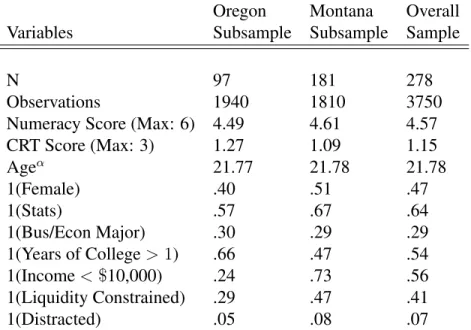
Participants 42
Stochastic Choice 44
Value Function 46
Scalar and Systematically-Varying Parameters 47
Maximum Likelihood Estimation 51
V. Results 53
Specifications with Homogeneous Preferences 53
Introducing Heterogeneous into the Value Function (via r) 55
Introducing Heterogeneous into the Weighting Function 56
Comparision of Common Specifications and Lorenz Curve Specification 60
VI. Conclusion 62
VII. Appendix 65
VIII. Glossary 75
v
List of Figures
Figure 1: The Tversky and Kahneman (1992) Probability Weighting Function 4 Figure 2: Commonly Used One-Parameter Probability Weighting Functions 6
Figure 3: The Tversky and Kahneman (1992) Value Function 9
Figure 4: Marginal Weight Contribution of Outcome Probability pi to Rank ri 11
Figure 5: A Lorenz Cruve with k = 2 26
Figure 6: A Lorenz Curve Mirrored at Each Axis 29
Figure 7: Commonly Used Two-Parameter Probability Weighting Functions 33 Figure 8: The Effect of Shifting the Fixed Point Parameter m, fixing s and a 35 Figure 9: The Effect of Shifting the First Shape Parameter s, fixing m and a 36 Figure 10: The Effect of Shifting the Second Shape Parameter a, fixing m and s 37
Figure 11: Amplification and Dampening along the Left Curve 38
Figure 12: The Limiting Functional Form as the Second Shape Parameter a → -∞ 39
vi
List of Tables
Table 1: Holt and Laury Multiple Price List 65
Table 2: Summary Statistics 66
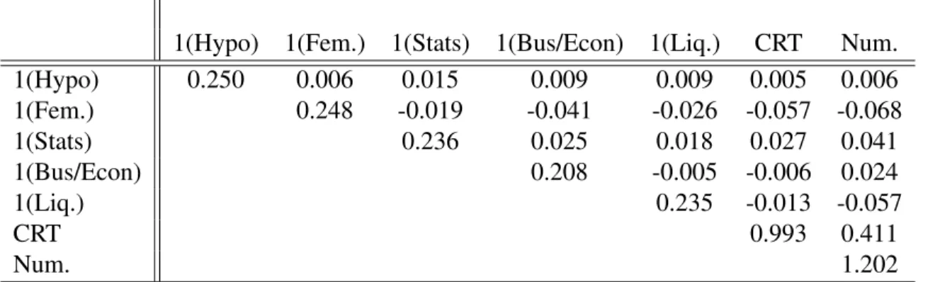
Table 3: Variance Covariance Matrix for the Seven Candidate Variables 67
Table 4: Estimation with All Scalar Paramaters 68
Table 5: Estimation with Systematically-Varying Parameter r 69
Table 6: Estimation with Systematically-Varying Parameters r and s 70 Table 7: Estimation with Systematically-Varying Parameters r, s, and a 71 Table 8: Estimation with Systematically-Varying Parameters r, s, and m. Fix a = 0 72 Table 9: Criterion Scores among Lorenz Curve Weighting Function Specifications 73 Table 10: AIC among Specifications with Heterogeneous Weighting Functions 74
I. Introduction
Probability Estimation versus Probability Weighting
Individuals tend to overestimate vastly the probability of rare events such as nuclear accidents, plane crashes, or terrorist attacks and to underestimate the probability of com-mon events such as heart disease or car accidents [Armantier (2006); Hakes and Viscusi (2004); Lichtenstein et al. (1978); and Viscusi, Hakes, and Carlin (1997)]. These types of distortions of objective probabilities into probability estimates occur because we perceive events as more or less likely to occur than they actually are. When the probabilities of possible consequences are unknown, decisions must be made under uncertainty.
Distortions can occur even when a decision maker has full awareness of the objec-tive probability distribution. For example, people purchase lottery tickets even though most know that the chances of winning are extremely low [Burns, Chui, and Wu (2010)]. With-out a notion of distorting probabilities into decision weights, it is difficult to reconcile the facts that people buy lottery tickets and insurance. Decision weights measure the attention or importance given to outcomes, and not merely the perceived likelihood that the out-comes will occur. When the probabilities of possible consequences are actually known, decisions must be made under risk. Decision-making under uncertainty contains the subset of decision-making under risk. Given an uncertain decision, an agent can distort the un-known probabilities into probability estimates and then distort those probability estimates
into decision weights. We focus on probability weighting of decisions under risk and not probability estimation of decisions under uncertainty. This example from Richard Zeckhauser, reported in Kahneman and Tversky (1979), illustrates individuals’ nonlinear weighting of probabilities:
Suppose you are compelled to play Russian roulette, but are given the opportunity to purchase the removal of one bullet from the loaded gun. Would you pay as much to reduce the number of bul-lets from four to three as you would to reduce the number of bulbul-lets from one to zero?
In general, people would pay more to reduce the number of bullets from one to zero, ensuring certain survival, than from four to three. The psychological impact of a change in probability from1/6to0is greater than a change from4/6to3/6. Conversely, most people would pay more to reduce the number of bullets from six to five, avoiding certain death, than from four to three. Whereas human instinct dictates that the reduction of bullets from one to zero has greater value than the reduction of bullets from four to three, economic theory dictates the opposite conclusion, where the value of money is reduced by the considerable probability that one will not live to enjoy it (i.e., the marginal utility of assets is greater in life than in death). A rational agent would weight each outcome by equal probability but would be willing to pay more for life-saving measures as the probability of her death increases. Tversky and Kahneman (1992) established a psychological hypothesis for this distortion: individuals are sensitive to a reference point and become less sensitive to changes in probability as they move away from that reference point. The endpoints of the probability domain, 1 and 0, act as reference points because they represent the certainty that a particular event will or will not happen.
The Probability Weighting Function
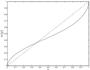
The psychological literature has considered the probability weighting function, a model of probability distortion, since the studies of Preston and Baratta (1948) and Ed-wards (1954). Renewed interest in the function emerged from the economics literature with the work of Handa (1977) and Kahneman and Tversky (1979). The probability weighting functionw : [0,1] →[0,1]takes the objective probabilitypas its argument and distorts it into a transformed probabilityw(p), which better describes the psychological consequences of risky events. The function increases on[0,1]and restricts the endpoints tow(0) = 0and w(1) = 1. If, for a given agent,w(p) =pfor the entire probability domain, then that agent assigns weights to all events equal to their corresponding objective probabilities. This case of linear probability weighting represents a baseline case against which all probability distortions will be compared. Therefore, the identity line accompanies each plot of the weighting function.
From experimental testing on the properties of the weighting function, the dominant result is that w(·) has a “regression” relative to the identity line, a fixed point near p = 1/3, and an inverse-S shape [Abdellaoui (2000); Abdellaoui, Bleichrodt, and L’Haridon (2007); Bleichrodt and Pinto (2000); Camerer and Ho (1994); Fox and Tversky (1995); Gonzalez and Wu (1999); Kahneman and Tversky (1979); Tversky and Kahneman (1992); and Wu and Gonzalez (1996, 1998)]. A regression of w(·) relative to the identity line means that people tend to overweight small probabilities,w(p) > p, and underweight the rest of the probability domain, w(p) < p. The point at which the weighting function
0 0.1 0.2 0.3 0.4 0.5 0.6 0.7 0.8 0.9 1 0 0.1 0.2 0.3 0.4 0.5 0.6 0.7 0.8 0.9 1 w ( p ) p
Figure 1: The Tversky and Kahneman (1992) Probability Weighting Function
The graph plotsw(·)withγ = 0.65. In the background lies the identity functionw(p) = p, which is a45o
line.
transitions from overweighting to underweighting, w(p) = p, is called the fixed point. A fixed point of p = 1/3 reflects the observation that the region of overweighting covers only one-third of the probability domain, whereas the region of underweighting covers the remaining two-thirds. An inverse-S shape for the probability weighting function means that w(·)begins as concave and then transitions into convexity. The change in curvature reflects people’s diminishing sensitivity to probability changes as they move away from either endpoint [Gonzalez and Wu (1999)]. An inverse-S-shaped weighting function could lie completely above or below the identity line, and a regressive weighting function need not start as concave and end as convex; hence, an inverse-S shape and regression relative to the identity line are logically independent properties. However, the region of overweighting (underweighting) usually does correspond to the region of concavity (convexity). Under this condition, the fixed point of the probability weighting function also acts as its inflection
point.
Over the course of numerous attempts to characterize the probability weighting func-tion, researchers have offered several simple parameterizations of its functional form. All of the common parameterizations ofw(·)capture its three main qualitative properties. The standard inverse-S-shaped probability weighting function, introduced by Tversky and Kah-neman (1992), is a function governed by a single parameter, γ, which controls both the curvature and the elevation of the function:
wT K(p) = p γ
[pγ+ (1−p)γ)]1/γ; if0.3≤γ ≤1 (1)
Although this specification is common, a normative case for adopting it has not been made [Cavagnaro et al. (2013)]. The LinLog two-parameter specification resembles Tversky and Kahneman’s one-parameter version. The LinLog specification is based on the assumption of a linear relationship between the log of the weighting odds and the log of probability odds:
ln( w(p)
1−w(p)) =γln(
p
1−p) +ln(δ) Some rearrangement yields,
w(p)LL = δp γ
δpγ+ (1−p)γ; if0< γ, δ (2)
Goldstein and Einhorn (1987) originally used this functional form, but not explicitly as a probability weighting function. Gonzalez and Wu (1999) argued for its appeal because it captures two properties to be discussed below: attractiveness and discriminability. In
contrast, Prelec (1998) derives his two-parameter probability weighting function based on the three axioms of compound invariance, subproportionality, and diagonal concavity:
w(p)P II =exp(−δ(−lnp)γ); if0< γ ≤1, 0< δ (3) The one-parameter Prelec function is obtained by settingδto unity:
w(p)P I =exp(−(−lnp)γ); if0< γ ≤1 (4) Each of these specifications of the probability weighting function nests the most simple case of linear weighting,w(p) =p, whenγ, δ = 1.
0 0.1 0.2 0.3 0.4 0.5 0.6 0.7 0.8 0.9 1 0 0.1 0.2 0.3 0.4 0.5 0.6 0.7 0.8 0.9 1
w
(
p
)
T K w ( p ) p 0 0.1 0.2 0.3 0.4 0.5 0.6 0.7 0.8 0.9 1 0 0.1 0.2 0.3 0.4 0.5 0.6 0.7 0.8 0.9 1w
(
p
)
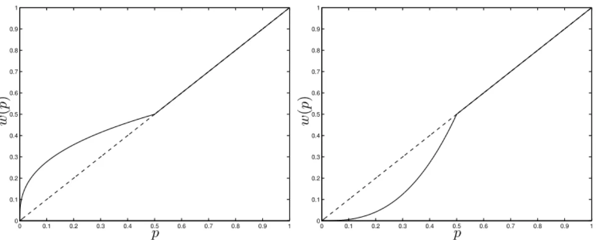
P I w ( p ) p Figure 2: Commonly Used One-Parameter Probability Weighting FunctionsTwo families of functions have been commonly used as probability weighting functions. The two functions are plotted for a range of parameter values. Left: the Tversky and Kahneman (1992) function forγ=0.2 to 1, in increments of 0.1. Right: the Prelec-1 function forγ=0.1 to 1, in increments of 0.1.
Decision-Making Under Risk
So far we have distinguished between two types of probability distortions: proba-bility estimation and probaproba-bility weighting. We have also reviewed the common ways in
which researchers model probability weighting. Probability distortion plays an important role in several strands of research, including visual frequency estimation, frequency estima-tion based on memory, confidence rating, signal detecestima-tion theory, decision-making under risk, and decision-making under uncertainty.1 Our study of probability distortions will take place in the context of decision-making under risk.
Decisions under risk involve evaluating one or more gambles with known outcomes and probabilities. A simple gamble g= (y1, p1;y2, p2;...;yN, pN)is a probability
distribu-tion, where yn is the monetary or non-monetary payoff from thenth outcome with
proba-bilitypn of occurring. The first theoretical attempt to evaluate these gambles was
formu-lated by Daniel Bernoulli (1738) and then axiomatized by von Neumann and Morgenstern (1944). Their approach to decision-making under risk derives from axioms of rational behavior and is known as expected utility theory (EUT). The experiments we use in our illustration involve only two-outcome gambles with positive payoffs. Thus, we will restrict our discussion to this case. Suppose an individual can choose either gamble gA, with a50%
chance of$200and a50%chance of only$100, or gamble gB, with a20%chance of$800
and an80%change of only$10. Under EUT, the individual would choose the gamble with the larger expected utility:
U(gA) =.5·u(W + $200) +.5·u(W + $100)and U(gB) =.2·u(W + $800) +.8·u(W + $10),
where W is current wealth and u(·) is an increasing utility function exhibiting either 1
concavity or convexity. Under EUT, individuals weight outcomes by their correspond-ing objective probabilities, implycorrespond-ing a probability weightcorrespond-ing function of w(p) = pfor all p∈[0,1].
In contrast to EUT (and its characterization of how a rational agent should gamble), prospect theory attempts to describe how an agent actually gambles. Tversky and Kahne-man’s (1992) cumulative prospect theory (CPT) introduces some important deviations from expected utility theory. Prospect theory is still regarded as the best description of how people evaluate risk in experimental settings [Barberis (2013)]. Research over the last decade has attempted to apply prospect theory to various economic settings. In fields where attitudes toward risk play a central role, such as in finance and insurance, CPT has clear applications. For example, can we explain the cross section of average returns using a model in which investors evaluate risk in a psychologically more realistic way? Behavioral finance has been a highly fruitful line of inquiry in the recent literature. Prospect theory has been applied to answer questions related to the endowment effect, industrial organization, labor supply, and consumption-savings decisions. Kahneman and Tversky’s (1979) original formulation of prospect theory evaluates the gambles in our example as
V(gA) =w(.5)·v($200) +w(.5)·v($100)
V(gB) =w(.2)·v($800) +w(.8)·v($10),
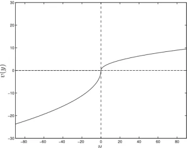
where v(·), termed the value function, is increasing and v(0) = 0. The value function describes how an individual values any possible payoff. This original prospect theory for-mulation poses two problems: it may violate stochastic dominance and it implies that the
decision weight depends only on the probability of the outcome and not on the outcome itself. −80 −60 −40 −20 0 20 40 60 80 −30 −20 −10 0 10 20 30 v ( y ) y
Figure 3: The Tversky and Kahneman (1992) Value Function
A plot of the value function proposed by Tversky and Kahneman (1992), wherev(y) = yκ wheny <0andv(y) =−λ(−y)κ
wheny≥0andyis the dollar gain or loss. Hereκ= 0.5
andλ= 2.5.
To resolve the theoretical limitations of original prospect theory, a decision-making theory must incorporate rank dependence. CPT is the most popular of the so-called rank dependent models, which acknowledge that the attention given to an outcome depends not only on the probability of the outcome but also the favorability of the outcome in comparison to the other possible outcomes in the gamble [Diecidue and Wakker (2001)]. Rank dependent models order outcomes in the gamble g= (y1, p1;y2, p2;...;yN, pN)from
best to worst: y1 > y2 > · · · > yn. Suppose we own a gamble gC = ($80, 1/5; $60,
1/5; $40, 1/5; $20, 1/5; $0, 1/5). It would be good news to receive information that the gamble will have a payoff more than$20. The probability of receiving more than$20,3/5, is the good-news probability or rank of the$20outcome. The rank of a specific outcomeyi,
ri =p1+·+pi−1, describes the probability of the gamble yielding an outcome ranked better thanyi. The ranks of outcomes$80, $60, $40, $20, and$0are0, 1/5, 2/5, 3/5, and4/5,
respectively—the lower the rank, the better the outcome. Rank dependent models apply the probability weighting function to the cumulative probability (i.e., the rank) rather than to the outcome probability. The decision weightπi of outcomeyi is the difference between
the weighted rank of the next best alternative outcome,yi+1, and the weighted rank of the outcome,yi:
πi =w(p1 +·+pi)−w(p1+·+pi−1) =w(ri+1)−w(ri) (5)
In particular,π1 = w(p1). The decision weight is the marginal contribution, measured in w(·)units, of the outcome probability to the rank. The decision weightπiincorporates both
the outcome probability,pi, and the outcome’s relative favorability within the gamble.
Whereas the probability weighting function describes how people weight cumulative probabilities in their minds, thedecision weightdescribes how people weight outcomes in their decision-making under risk. The divergence between the two concepts stems from the fact that people weight each outcome not just by its weighted cumulative probability, but also by how its weighted cumulative probability compares to the weighted cumulative probability of the next best outcome. The probability weighting functionw(·)is a “good-news” weighting function because it transforms the ranks.2 Under CPT, people evaluate
2
gambles as V(g) = n X i=1 πi·v(yi) (6)
Returning to our original example, under CPT, the individual would choose between gam-bles gAand gBaccording to the largest expected prospect value ofV(gA)andV(gB):
V(gA) =w(.5)·v($200) + [1−w(.5)]·v($100) V(gB) =w(.2)·v($800) + [1−w(.2)]·v($10) 0 0.1 0.2 0.3 0.4 0.5 0.6 0.7 0.8 0.9 1 0 0.1 0.2 0.3 0.4 0.5 0.6 0.7 0.8 0.9 1 ri | | | | | | | | w(ri) −− − − − − − −↑ πi pi → ri+pi | | | | | | | | | | w(ri +pi) −− − − − − − − − − − − w ( p ) p
Figure 4: Marginal Weight Contribution of Outcome Probabilitypito Rankri
Here we see the interaction between the weighting functionw(·)and the decision weightπ under rank dependence. The rank for outcomeyiisri=p1+·+pi−1.
Prospect theory captures four generalizations of EUT: reference dependence, loss aversion, diminishing sensitivity, and probability weighting. Both the utility function and the value function increase in the preference an individual has for an outcome. The cur-vature of each function represents an individual’s risk preferences over that domain of
outcomes. Reference dependence suggests that people make decisions based on changes
in attributes, as opposed to their absolute magnitudes. In CPT people derive prospect value from gains and losses, measured relative to some reference point, typically the status quo, rather than from absolute levels of wealth. This implies that the argument ofv(·)isyrather thanW+y. Loss aversion means that people are more sensitive to losses than to gains of the same magnitude. The value function generates this property by being steeper in the region of losses than in the region of gains. People tend to be risk averse with respect to gains and risk loving with respect to losses. Diminishing sensitivity to changes in wealth suggests that the value function is concave in the region of gains and convex in the region of losses. In contrast, any utility function imposes the same curvature for all wealth levels, so that risk preferences cannot switch between risk aversion and risk affinity. Unlike EUT, CPT allows for a nonlinear probability weighting function and this function can differ between losses and gains.3 Our experiment contains only gains, however, so our modeling does not need to incorporate loss aversion, diminishing sensitivity to losses, or a loss-specific probability weighting function.
Further psychological interpretations of the probability weighting function derive from the CPT framework. One person’s weighting function w1(·)is said to be more ele-vated than another’sw2(·)ifw1(p)≥w2(p)for allp∈[0,1]with at least one point of strict inequality. In the context of CPT with two-outcome gambles that pay only gains, a weight-ing function that is more elevated will assign greater weight to the more favorable outcome. Gonzalez and Wu (1999) interpret an interpersonal difference in elevation between
weight-3
ing functions as relative attractiveness. One person finds betting on the chance domain more attractive than a second person. Elevation can differ between chance domains as well as across individuals. An individual may prefer to bet on stock prices rather than on the outcomes of baseball games, for example, holding constant the chance of winning. Gon-zalez and Wu (1999) link the curvature of the weighting function, implied by diminishing sensitivity, to the psychological concept of discriminability. Recall that individuals exhibit sensitivity to the probability changes near the two endpoints of the probability domain (i.e., 0 and 1), and this sensitivity to probability changes diminishes as they move away from the endpoints. A person with a EUT weighting function ofw(p) =pfor allp∈[0,1]exhibits a perfect ability to discriminate a1%probability change. Conversely, a person with a near horizontal weighting function and extreme steepness near the two endpoints exhibits low ability to discriminate a1%probability change.
Although Gonzalez and Wu’s (1999) psychological interpretation characterizes the weighting function as a whole, it does not adequately interpret the psychological difference between the concave overweighted region (i.e., the “bulge”) and the convex underweighted region (i.e., the “sag”). Wakker (1994, 2008) and Diecidue and Wakker (2001) prove that convexity in a weighting function reflects probabilistic risk aversion or pessimism. Like-wise, they prove that concavity in a weighting function reflects probabilistic risk affinity or optimism. The decision weight for an outcome, which depends on the weighting func-tion’s differences, will be affected by the slope rather than absolute level ofw(·). Hence, a change in the slope of the decision weight implies a change in the curvature (i.e., the slope of decision weight’s slopes) of the weighting function. Pessimism is present if worsening
the rankrof outcomexincreases its decision weight (i.e., the worst outcomes receive rela-tively more decision weight than less bad outcomes). Specifically,π(p) = w(r+p)−w(r)
is decreasing inr if and only ifw(·)is convex. Optimism is present if improving the rank r increases the decision weight (i.e., the best outcomes receive relatively more decision weight than less good outcomes). Analogously,π(p) =w(r+p)−w(r)is increasing inr if and only ifw(·)is concave.
Recall that the weighting function transforms the cumulative probability (i.e., rank) of each outcome. A large cumulative probability for outcome xi, where its rank ri =
p1+· · ·+pi−1, corresponds with an unfavorable outcome relative to other outcomes. There
is a large probability that the gamble will yield a better outcome thanxi sinceri is large,
which means xi has a relatively bad rank compared to other outcomes. A small
cumu-lative probability for outcome xi corresponds with a favorable outcome relative to other
outcomes. There is a small probability that the gamble will yield a better outcome thanxi
sinceri is small, which means xi has a relatively good rank compared to other outcomes.
Therefore, as the rank of an outcome worsens (i.e., the cumulative probability increases), its decision weight is determined by a region of the weighting function that is farther away fromw(0) = 0and closer tow(1) = 1.
Concavity ofw(·), or optimism, for small cumulative probabilities implies that the most favorable outcomes are overweighted. Within the favorable outcome domain of small cumulative probabilities, shifting to better-ranked outcomes, according to optimism, in-creases the decision weight. Convexity ofw(·), or pessimism, for large cumulative proba-bilities implies that the least favorable outcomes are also overweighted. Within the
unfavor-able outcome domain of large cumulative probabilities, shifting to worse-ranked outcomes, according to pessimism, increases the decision weight. Little attention or weight is given to intermediate outcomes [Quiggin (1982) and Weber (1994)]. Choices in our framework are discrete and not continuous, so the absolute level of the weighting function does im-pact probabilistic risk preferences. Overweighting (underweighting) intensfies the degree of optimism (pessimism). The inflection point of the weighting function separates the prob-ability domain into a region of probabilistic risk affinity and a region of probabilistic risk aversion.
The common parameterizations of the probability weighting function do not per-mit independent estimation of the fixed point. An elevated weighting function indicates a higher fixed point. A higher fixed point implies an elevated weighting function holding constant the curvature parameter, under the common parameterizations. Hence, the eleva-tion parameter controls the fixed point, but not independently from the other parameters. The Prelec-1 weighting function has its fixed point at 1/e. The Tversky and Kahneman (1992) single-parameter weighting function necessarily confounds the estimation of the fixed point and curvature. The formula for the Prelec-2 fixed point is given by
p∗ =exp(−δ1/(1−γ))with0< γ≤1, 0< δ
Hence, the fixed point collapses to1/ewhenδ= 1. The formula for the fixed point of the LinLog weighting function is given by
p∗ = δ
1/(1−γ)
Both of the common two-parameter probability weighting functions thus have fixed points that depend on both parameters. This dependence prevents clear hypothesis testing of the location of the fixed point. We introduce a three-parameter probability weighting function that does allow for independent estimation of the fixed point; the fixed point depends on its own parameter. In fact, our alternative model allows for the case that an individual’s probability weighting function may never cross the identity line within the interior of the probability domain. To the extent that the region of concavity (convexity) corresponds to the region of overweighting (underweighting), the fixed point acts as the inflection point forw(·). Pinning down the location of the fixed point has theoretical value for fields such as economics and psychology because this point approximates where probabilistic risk attitudes transition from risk affinity to risk aversion along the probability domain.
All of the common weighting function parameterizations, furthermore, contain only one curvature parameter. Given that the typical empirical probability weighing function with an interior fixed point has an inverse-S shape, with two distinct regions, a single cur-vature parameter may be overly restrictive. A natural concern with the empirical estimation of these models is whether the estimated shape may be an artifact of the functional form in one region and not fully reflective of actual probability risk preferences throughout the domain. Our alternative function estimates the bulge to the left of the fixed point indepen-dently from the sag to the right of the fixed point. That is, we allow for separate estimates of the degree of optimism and pessimism across the probability domain. Individuals may significantly overweight the most favorable outcomes more than they overweight the most unfavorable outcomes, or vice versa.
Finally, we test our three-parameter function in a rich setting that seems not to have received adequate attention in the literature. Most studies concerning decision-making un-der risk emphasize the utility or value function component v(·). The few studies that do focus on the weighting function, w(·)often exclude heterogeneity in preferences. That is, all subjects are constrained to have approximately the same underlying preferences and the same weighting function. However, the representative individual’s probability weighting function may not adequately capture each individual’s weighting function. We generalize the probability weighting function to allow for heterogeneity across various sociodemo-graphic variables. The available observable sociodemosociodemo-graphic variables may be proxies for unobservable factors that influence probability weighting behavior. We will test whether groups formed on the basis of a number of sociodemographic variables exhibit systematic differences in the parameter values of their estimated probability weighting functions.
II. Literature Review
Parameteric and Nonparametric Methods
Any parametric model of decision-making under risk necessarily makes at least three assumptions about functional form for the components of the model: (1) the utility or value function, v(·); (2) the probability weighting function, w(·); and (3) the combination rule (e.g., expected utility theory, original prospect theory, or cumulative prospect theory) that combines the first two components,w(p1)·v(y1) + [1−w(p1)]·v(y2). The challenge in identifying these forms stems from the fact that they cannot be estimated directly. Instead, they must be inferred from people’s observed choice behavior. The standard technique of assuming specific functional forms forv(·)andw(·)has the limitation that there is no way to assess independently the fit ofv(·)andw(·).4 Stott (2006) finds that the performance of any standard one- and two-parameter weighting function depends on assumptions about the other component functions in cumulative prospect theory, including the value function and choice function. When the surrounding functions within which the weighting function is embedded have a worse fit, the extra flexibility provided by the parameter in the weighting function may play a compensating role.
The methodological limitation of parametric methods, that there is no way to assess the fit of each component function separately, has driven some researchers to explore non-parametric specifications for the probability weighting function. Nonnon-parametric methods make no particular assumption about the forms of v(·) andw(·) other than the
combina-4
For examples of the standard technique see Camerer and Ho (1994), Hey and Orme (1994), Tversky and Fox (1995), and Tversky and Kahneman (1992).
tion rule, so that each component function can be assessed separately. Both parametric and nonparametric methods can estimate the component functions at either the aggregate level or the individual level. For an aggregate weighting function, the data are averaged across participants according to a single-agent stochastic choice model, suppressing any hetero-geneity in preferences. A representative agent model can be generalized to allow for het-erogeneity in preferences by varying parameters systematically with observable variables. The weighting function will still be an aggregate weighting function, but an aggregate func-tion for each differentiated observable group rather than an aggregate of the whole sample. Alternatively, estimation of individual weighting functions allows for each individual to have a separate weighting function. Depending on whether the estimation uses parameteric or nonparameteric methods, individual weighting functions are reflected by either unique parameter estimates for each individual or separate point estimates for each individual. Few studies actually test the weighting function at the individual level because this type of test requires an inordinate amount of data on the choice behavior of each individual.
Studies using nonparametric methods adopt one of two main research strategies. The first strategy obtains information about the qualitative properties of the weighting function by testing simple preferences conditions. These studies test the weighting function at the aggregate level. Currim and Sarin (1989) confirm underweighting, subproportionality, and convexity ofw(·)in the aggregate. Wu and Gonzalez (1996, 1998) find aggregate behavior consistent with an inverse-S-shaped weighting function. The second strategy consists of eliciting point estimates for each individual’s probability weighting function throughout the probability interval. Wakker and Deneffe (1996) first propose a trade-off method to
elicit preference functions nonparametrically. Gonzalez and Wu (1999), Abdellaoui (2000), and Bleichrodt and Pinto (2000) all follow this second strategy. Their results demonstrate significant heterogeneity in the weighting function at the individual level that is not likely to be explained purely as noise.
Bleichrodt and Pinto (2000) confirm the robustness of nonlinear probability weight-ing in a medical context. Participants are assigned a hypothetical disease and they have to choose between disease treatments before it was known which disease they actually have. Outcomes of treatments are expressed in terms of expected remaining life-years. The non-parametric studies have limited sample sizes because they elicit, for each individual, many choices for each probability level and for each outcome level. The study by Gonzalez and Wu (1999) elicitswi(·)at eleven probability levels but has a sample size of only ten
indi-viduals. The studies by Abdellaoui (2000) and Bleichrodt and Pinto (2000) have sample sizes of forty and forty-nine, but elicitwi(·)at only five probability levels. Although these studies do confirm that preference heterogeneity exists, the samples are too homogeneous (i.e., all participants were graduate students or undergraduates in economics) and too small to characterize how risk attitudes may vary systematically with observed characteristics of individuals across the general population.
Nonparametric studies typically constrain the number of subjects in the study too severely to permit a full characterization of the distribution of risk preferences in the pop-ulation. However, these studies have taught us that any parametric study concerning sys-tematic heterogeneity inwi(·)across individualsi = 1,2, . . . , nor groupsj = 1,2, . . . , J must employ a fairly flexible parametric form. Little is known about the distribution of risk
preferences in the population.
The Distribution of Probability Risk Preferences
Harbaugh, Krause, and Vesterlund (2002), using the Prelec-2 weighting function, investigate how risk attitudes change with age. They find that children’s choices are ac-tually consistent with the underweighting of low-probability events and the overweighting of high-probability ones (i.e., the opposite of the pattern predicted by cumulative prospect theory). This tendency diminishes with age until the point that adults appear to use the objective probability when evaluating risk prospects (i.e., the EUT weighting function).
Fehr-Duda, de Gennaro, and Schubert (2006) use the LinLog two-parameter proba-bility function to study the relationship between gender and risk-taking behavior. They find that women tend to underweight large probabilities of gains more strongly than men do. Women appear to be more risk-averse than men when decisions are framed in investment terms. Bruhin, Fehr-Duda, and Epper (2010) use the same probability weighting function as Fehr-Duda et al. (2006) and find two classes of individuals in their data sets. Eighty percent of the subjects exhibit significant departures from linear probability weighting, consistent with CPT, and twenty percent of the subjects weight probabilities approximately linearly, consistent with EUT. The only variable that consistently affects behavioral parameters be-tween the groups is an indicator for gender. Within the study, women have a substantially lower value ofγ (i.e., aw(·)that is flatter in the region of medium probabilities and steeper near the ends) than men. They conclude that women tend to be less sensitive to changes in probability than men.
The above papers have been experimental studies, but Donkers, Melenberg, and Van Soest (2001) analyze a large, representative set of Dutch survey data that contains infor-mation on respondents’ risk attitudes as well as background inforinfor-mation on each person. Their semiparametric model does not specify v(·)or w(·), but makes a minimal assump-tion about the choice funcassump-tionP(V(gR), V(gS)|x), a function that indicates the probability that an individual will choose the risky gamble over the safe gamble. The choice function reflects the empirical finding that decision-making has a random component. They assume that the expected prospect values, V(gR) and V(gS), depend on an index, x′β, where x
is a vector of observable individual characteristics. Vector β is the vector of parameter values to be estimated. They do not specify how the index influences each component function ofV(·). Specifically, they assume a higher index valuex′β implies a larger value
of P(V(gR), V(gS)|x), which they argue is an indication of greater risk aversion. The semiparametric estimation results show a significant relationship between the subjects’ es-timated degree of risk aversion and their age, gender, education level, and income.
The generality of the semiparametric model, in that it identifies only the choice func-tionP(V(gR), V(gS)|x)rather than its component functions, prevents an interpretation of the effects of differences in risk attitudes on v(·)or w(·), more generally. Moreover, the semiparametric estimation results indicate that a single index (i.e., one systematically vary-ing parameter) is too restrictive. Hence, Donkers et al. (2001) form a parametric model with a first index,x′β
v, to control for variation in the value function, and a second index,
x′β
w, to control for variation in a Prelec-1 probability weighting function. They find that the
wealth, and marital and employment status. The estimated index,x′β, in the
semiparamet-ric model of the Donkers et al. (2001) paper closely resembles the estimated value of the differentiated index, x′β
v, in the value function rather than the estimated index, x′βw, in
the probability weighting function. The semiparametric estimation suggests two key con-clusions for any parametric study concerning heterogeneity in the weighting function: (1) parametric models of decision-making under risk should embody at least two indexes, and (2) heterogeneity inw(·)should be permitted to be distinct from heterogeneity inv(·).
Best Parametric Form for the Probability Weighting Function
Another related line of research endeavors to find the “best” parametric form for w(·). The trade-off pits the desire for a parsimonious form against the desire for a good fit to the data. Studies within this line of research essentially set up a “horse race” between the common probability weighting functions [Abdellaoui (2000), Bleichrodt and Pinto (2000), Cavagnaro et al. (2013), Gonzalez and Wu (1999), Stott (2006), and Zhang and Mal-oney (2012)]. For example, Abdellaoui (2000), Bleichrodt and Pinto (2000), and Gonzalez and Wu (1999) elicit their nonparametric point estimates of each individual’s probability weighting function and use nonlinear least squares estimation to fit the standard parametric weighting functions to these point estimates. All three of the studies also fit parametric functions to the median point estimates (i.e., the median certainty equivalent for each prob-ability level) using nonlinear least squares. These parametric estimates on the median data characterize the aggregate probability weighting function in sense that the central tendency of the sample’s choices describes the behavior of a representative agent. Bleichrodt and
Pinto (2000) and Gonzalez and Wu (1999) find that standard two-parameter functions fit the data much better than the standard one-parameter functions at the individual participant level, but only slightly better at the aggregate level. Gonzalez and Wu (1999) favor the two-parameter LinLog function for its psychological interpretation. Stott (2006) favors the Prelec-1 function, but only when paired with a power value functionv(y) = yλand a Logit
choice function. Cavagnaro et al. (2013) find heterogeneity in the best two-parameter form; some individuals are best described by a LinLog function while other are best described by a Prelec-2 form. Each of these studies discriminates among the standard small set of one-and two-parameter functional forms. They do not consider any three-parameter forms one-and cannot discriminate among the set of all possible parametric forms.
Two-parameter models of w(·) control elevation and curvature. The empirical evi-dence suggests that w(·)may have two separate regions: an overweighted concave curve (i.e., the “bulge”) and, after crossing the diagonal, an underweighted convex curve (i.e., the “sag”). The one- and two-parameter models combine all of the curvature information into a single parameterγ. However, it may be the case that the bulge and sag have inde-pendent magnitudes. In that case, an additional parameter would be needed. According to Cavagnaro et al. (2013), they would have strictly favored the LinLog model but some exaggerated overweighting of low probabilities by a subset of participants required that the analysis resort to the Prelec-2 form for some individuals. Perhaps the need for two separate two-parameter functions to best describe the individual probability weighting curvature in-dicates that the individual data are best captured by an even more general parametric form. Our three-parameter specification of w(·) allows for independent estimation of the bulge
and the sag as well as direct estimation of the fixed point. This additional flexibility an-swers the question of whether individuals are more sensitive to probability changes for lower- versus higher-cumulative-probability events.
Aggregate choice data seem to be well-characterized by a one-parameter functional form for w(·). At the individual level, however, a more-flexible form is needed to cap-ture heterogeneity in the shape and specification of w(·). Although our study does not seek to elicit the probability weighting function at the individual level, it does permit the representative agent’s weighting function to vary across sociodemographic groups. These observable individual characteristics might be correlated with unobservable characteristics that influence individual risk preferences. Hence, our systematically varying weighting function might require the same degree of flexibility as a weighting function wi(·) that
varies across each individual. Testing our specification of w(·)at the group level for het-erogeneity will (1) add to the relatively sparse literature on the distribution of risk attitudes and (2) identify the types of environments where a more-general parameterization of the weighting function may be appropriate.
III. Framework
Derivation of a Weighting Function Based on Lorenz Curve Forms
In welfare economics, a Lorenz curve is a cumulative plot of the share of income or wealth that is owned by the cumulative segment of the population. Lorenz curves have applications in describing problems in ecology, biodiversity, and physics. A Lorenz curve takes the form:
w∗ = 1−(1−p∗)1−1/k if1< k
The restriction on parameterk ensures convexity.
0 0.1 0.2 0.3 0.4 0.5 0.6 0.7 0.8 0.9 1 0 0.1 0.2 0.3 0.4 0.5 0.6 0.7 0.8 0.9 1 w ∗( p ∗) p∗
Figure 5: A Lorenz Curve withk= 2
Lopes (1984) argues for the intuitive value of Lorenz curves in capturing the psycho-logical features of decision-making under risk. She proposes that even if presented with a gamble in terms of outcome probabilities, people process probabilities in terms of their cu-mulative probabilities. The cucu-mulative character of Lorenz curves allows for representing
gambles in these cumulative terms. For a given gamble, she would order outcomes from worst to best. Then she plots the cumulative probability of receiving a particular outcome or worse on the x-axis and the cumulative proportion of expected value of a particular out-come or worse on the y-axis. The plot resembles a Lorenz curve. The plot can be seen as the cumulative proportion of the expected value accruing to cumulative segments of the population if the gamble is independently repeated for a large number of individuals.
The diagonal of a Lopes-Lorenz curve corresponds to a “sure thing,” a gamble with
100%probability of a single payoff. Hence, the expected value of each outcome or worse accrues evenly across the cumulative population segments in repeated trials. The degree of convexity, or deviation from the diagonal, indicates the amount of probability dispersion across outcomes, and it captures cases where the expected value accrues unevenly across members of the population. In a Lopes-Lorenz curve, the low end of the distribution cor-responds with the worst outcomes. She argues that just as welfare economists emphasize the condition of those who are least well-off in judging inequality, decision-makers have increased decision weights for outcomes at the low end of the distribution in judging risk. Her argument for “the distributional model” is equivalent to an argument for what we now call rank dependence.5
In the same spirit as Lopes (1984) argues for the intuitive value of Lorenz curves in modeling rank dependence, we argue for the intuitive value of Lorenz curves in modeling the probability weighting function. The Lorenz curve has some properties that make it
5
As a brief aside, Lopes orders outcomes and cumulative probabilities from worst to best, whereas mod-ern rank dependence orders them from best to worst.
attractive for modeling the sag portion of the probability weighting function. Mirroring the axes of the Lorenz curve will enable some functional form to be adapted to model the bulge portion of the probability weighting function as well. The attractive properties of Lorenz curves for our purposes include,
1. w∗ nest the linear case:w∗ = 1−(1−p) = pwhenk = 1
2. w∗ is continuous on[0,1]with range[0,1].
3. w∗ is increasing.
4. w∗(0) = 0andw∗(1) = 1.
5. w∗ is convex
6. w∗ lies at or below the diagonal.
7. w∗ transforms cumulative quantities
Within prospect theory, the diagonal serves as a benchmark case of EUT against which probability overweighting or underweighting may be measured. Within welfare economics, the diagonal corresponds to the Lorenz curve of a society in which everybody receives the same income and hence serves as a benchmark case against which actual in-come distributions may be measured. All of the properties listed above map nicely into the apparent empirical properties of portions ofw(·). The region ofw(·)to the right of its fixed point lies below the diagonal and is convex.
However unlike a Lorenz curve, w(·) contains a second region that lies above the diagonal and is concave. The fact that the Lorenz curve captures only the portion of the probability weighting function from the fixed point to p= 1 actually works to our advan-tage. If we mirror each axis of a typical Lorenz curve, we can achieve the desired properties
for the region of w(˙)to the left of the fixed point. We can construct the overall weighting function in a piecewise fashion by stitching together a mirrored Lorenz curve to the left of the fixed point and typical Lorenz curve to its right. The fixed point will become its own parameter. Allowing the Lorenz-type curvature parameter to differ to the left and right of the fixed point will permit separate estimation of the bulge and the sag. Other parameteri-zations cannot easily be adapted to separate the estimation of bulge from the sag because it is not straightforward how to subdividew(·)at the fixed point before that fixed point is defined. 0 0.1 0.2 0.3 0.4 0.5 0.6 0.7 0.8 0.9 1 0 0.1 0.2 0.3 0.4 0.5 0.6 0.7 0.8 0.9 1 w ∗( p ∗) p∗
Figure 6: A Lorenz Curve Mirrored at Each Axis
We transform w∗ from a curve that lies below the diagonal of a unit square into a
single-crossing function that might be suitable for describing w(·). Intuitively, we divide the weighting function into a piecewise function that transitions at the fixed pointm∗. We
the domain of the function so thatw∗is defined on[m∗,1]instead of[0,1]. w∗ = w−m ∗ 1−m∗ ,p ∗ = p−m ∗ 1−m∗ (7)
where wrepresents our weighting function and pits cumulative probability. Substituting the expressions forw∗ andp∗in terms ofwandpinto the Lorenz curve model produces:
w−m∗
1−m∗ = 1−(1−
p−m∗
1−m∗)
1−1/k ifp≥m∗ (8)
Rearrangement yields a function that describes the upper region of our piecewise function: w= 1−(1−m∗)(1− p−m∗
1−m∗)
1−1/k ifp≥m∗ (9)
Next we consider the lower region of the piecewise function. We use a mirrored version of the same shape. Replacingp∗ with (1−p∗)and w∗ with(1−w∗)will mirror
each axis. Now the underweighted convex curve becomes an overweighted concave curve:
(1−w∗) = 1−(1−(1−p∗))1−1/k (10)
w∗ = (p∗)1−1/k (11)
This time we change each variable so that the curve is defined on[0, m∗]instead of[0,1]:
w∗ = w
m∗ ,p ∗ = p
m∗ (12)
These expressions forw∗andp∗in terms ofwandpsubstituted into equation (11) produces:
w m∗ = ( p m∗) 1−1/k (13) w=m∗( p m∗) 1−1/k ifp < m∗ (14)
Our piecewise function now has one overweighted concave mirrored Lorenz curve to the left of the fixed point,m∗, and one underweighted convex Lorenz curve to its right:
w= m[mp∗]1−1/k ifp < m∗ 1−(1−m∗)(1− p−m 1−m∗)1−1/k ifp≥m∗ (15)
This function remains incomplete for two reasons. First, the magnitudes of the parameters are constrained, which will complicate their estimation. The fixed point parameter,m∗, is
constrained to the probability domain, [0,1]. Hence, we setm∗ = exp(m)/(1 +exp(m))
and estimate the unconstrained parameterm instead of m∗. Lorenz curves typically
con-strain the parameter k to (1,∞), or equivalently they constrain the exponent 1−1/k to the interval(0,1), so that the Lorenz curve cannot become either linear or concave. While this constraint holds for Lorenz curves used in welfare economics, the constraint does not apply to Lorenz curves used in probability weighting. In fact, the constraint is overly re-strictive for our purposes. Whenk → ∞, or equivalently when1−1/k = 1, our weighting function becomes linear. When k < 0, or equivalently when 1−1/k > 1 the function becomes S-shaped. The typical empirical weighting function follows an inverse-S shape. However, several studies have found cases in which the weighting function does follows a linear shape or even an S-shape [Barron and Erev (2003); Bleichrodt (2001); Goeree, Holt, and Palfrey (2002, 2003); Henrich and Mcelreath (2002); Humphrey and Verschoor (2004); Jullien and Salani´e (2000); Loomes (1991); Luce (1996); and Mosteller and Nogee (1951)]. Therefore, we replace the exponent 1−1/k withs∗ = exp(s). The constrained
parameter,s.
The second limitation of the new function so far is that it specifies only one shape parameter for both sides of the fixed point m∗. One motivation for this new specification
is to allow independent estimation of the bulge and the sag. We then solve this problem by permitting the shape parameter s to be scaled by a factor of a∗, but only beyond the
fixed point m∗. We actually estimate the logarithm of this factor a = ln(a∗)to constrain
the scale factor to be positive. Alternatively, if we scaled the constrained shape parameter s∗ by a factor of a∗, or equivalently added the unconstrained parameter a to the
uncon-strained parameters, then certain values forawould yield a perverse M-shape or W-shape that touches the diagonal once but never crosses. Multiplying the shape parameter sby a strictly positive factor a∗ prevents the possibility of this nonsensical pattern.
Incorporat-ing these generalizations yields our three-parameter Lorenz-type curve specification of the probability weighting function:
wLC(p|s, m, a) = m∗[ p m∗]exp(s) ifp < m∗ 1−(1−m∗)[1− p−m∗ 1−m∗]exp(sa ∗) ifp≥m∗ (16)
wherem∗ =exp(m)/(1 +exp(m))anda∗ =exp(a).
Properties of Weighting Function Based on Lorenz Curve Forms
This section provides intuition for how the parameters of our Lorenz curve probabil-ity weighting function control its form. To demonstrate its flexibilprobabil-ity, we first compare it with the most flexible of the common weighting functions, the two-parameter models. The fixed point has empirical value because it partitions where overweighting versus
under-0 0.1 0.2 0.3 0.4 0.5 0.6 0.7 0.8 0.9 1 0 0.1 0.2 0.3 0.4 0.5 0.6 0.7 0.8 0.9 1
w
(
p
)
LL w ( p ) p 0 0.1 0.2 0.3 0.4 0.5 0.6 0.7 0.8 0.9 1 0 0.1 0.2 0.3 0.4 0.5 0.6 0.7 0.8 0.9 1w
(
p
)
P II w ( p ) p Figure 7: Commonly Used Two-Parameter Probability Weighting FunctionsTwo families of two-parameter weighting functions. Left: The LinLog function forγ, δ=0.25 to 2, both in increments of 0.25. Right: The Prelec-2 function forγ=0.2 to 1,δ=0.4 to 2, both in increments of 0.2.
weighting occurs along the probability domain. If the fixed point equals the inflection point, then it also identifies where the transition from probabilistic risk affinity (i.e., concavity) to probabilistic risk aversion (i.e., convexity) occurs. Unlike its one-parameter counterpart which constrains the fixed point always to be equal to1/e, the Prelec-2 function allows the fixed point to vary. The LinLog form allows for flexibility in the estimation of the fixed point as well. However, both functions vary the location of the fixed point primarily as an artifact of varying the elevation of the entire curve.
Likewise, our function allows the fixed point to vary. As the fixed point parameter increases, so does the elevation of the entire curvature, holding fixed the shape parameters s and a. This implies that our fixed point parameterm∗ corresponds approximately with
the elevation parameter δof two-parameter models, when we hold fixed parameterssand a.
all. We estimate the underlying parameter m, which determines the fixed point bym∗ =
exp(m)/(1 +exp(m)). The function does not permit the values m∗ = 0 or m∗ = 1.
However, if no interior fixed point appears to exist, the function, in the limit asm → −∞
(or equivalentlym∗ →0), converges to a single Lorenz-type curve:
w(p|s, m=−∞, a) = 1−(1−p)exp(sa∗)
In the limit asm→ ∞(or equivalentlym∗ →1), our function yields the formula:
w(p|s, m=∞, a) =pexp(s)
If no interior fixed point exists, then the two curves degenerate into just one or the other. That is, the agent overweights or underweights the entire probability domain.
We now prove that the fixed pointm∗also acts an inflection point forw(·). The sign
of the second derivative of a function determine its curvature. When p∈(0, m∗), the sign
of the second derivative equals, sign[ ∂ 2 ∂p∂pw(p|s, m, a)] =sign[ m∗exp(s)(1−exp(s))( p m∗)exp(s) p2 ] =sign[s]
Whenp∈(m∗,1), the sign of the second derivative equals,
sign[ ∂ 2 ∂p∂pw(p|s, m, a)] =sign[ exp(a∗s)(exp(a∗s)−1)(1− p−m∗ 1−m∗)exp(a ∗s)−2 1−m∗ ] =sign[−a∗s] =−sign[s], sincea∗ >0
Only whens = 0, the linear case, does the weighting function have the same curvature on both sides of the fixed point. In general, the sign of curvature is opposite on either side of the fixed point. Thus, the fixed pointm∗ acts as the point at which curvature changes, the
inflection point. 0 0.1 0.2 0.3 0.4 0.5 0.6 0.7 0.8 0.9 1 0 0.1 0.2 0.3 0.4 0.5 0.6 0.7 0.8 0.9 1 w ( p ) p 0 0.1 0.2 0.3 0.4 0.5 0.6 0.7 0.8 0.9 1 0 0.1 0.2 0.3 0.4 0.5 0.6 0.7 0.8 0.9 1 w ( p ) p Figure 8: The Effect of Shifting the Fixed Point Parameterm, fixingsanda
Left:mvaries so thatm∗ =0.1 to 0.9 in increments of 0.1. Right: The limiting case ofmor
whenm∗= 1. Parameterss=−1anda= 0are held fixed.
Parameter s regulates the overall shape of the function. A negative sign on the pa-rameter s implies that the function will follow the predominant empirical pattern of an inverse-S shape. A positive sign implies an atypical S-shape. If parameter s equals zero, then the function degenerates to linear probability weighting. The greater the magnitude of the shape parameter, the greater the degree of curvature. The bulge becomes more con-cave and the sag becomes more convex. Hence, our overall shape parameterscorresponds roughly with the curvature parameterγof the LinLog and Prelec-2 functions, holding fixed the parametersmanda.
0 0.1 0.2 0.3 0.4 0.5 0.6 0.7 0.8 0.9 1 0 0.1 0.2 0.3 0.4 0.5 0.6 0.7 0.8 0.9 1 w ( p ) p 0 0.1 0.2 0.3 0.4 0.5 0.6 0.7 0.8 0.9 1 0 0.1 0.2 0.3 0.4 0.5 0.6 0.7 0.8 0.9 1 w ( p ) p Figure 9: The Effect of Shifting the First Shape Parameters, fixingmanda
Left: s =-1 to -0.1, in increments of 0.1. Right: s =from 0.1 to 1, in increments of 0.1. Parametersm= 0.4anda= 0are held fixed.
curve degenerates to a step function:
w(p|s=∞, m, a) = 0ifp < m∗ 1ifp≥m∗ w(p|s=−∞, m, a) =m∗
So far this Lorenz-curve-based weighting function resembles the two-parameter models that govern the elevation and curvature of w(·). Unlike the other functions though, our function independently estimates the fixed point. It does not conflate the estimation of the shape and the fixed point. An additional source of flexibility in our function comes from the third parameter.
Unlike other parameterizations that commingle the estimation of the two regions, our parameterization disentangles the estimation. This occurs through the interaction of the second shape parameter,a, with the first shape parameter,s, along only one side of the fixed point. The second shape parameter acts as an amplifier or dampener of the curvature
to the right of the fixed point relative to its left. Since the second shape parameter, a, acts 0 0.1 0.2 0.3 0.4 0.5 0.6 0.7 0.8 0.9 1 0 0.1 0.2 0.3 0.4 0.5 0.6 0.7 0.8 0.9 1 w ( p ) p 0 0.1 0.2 0.3 0.4 0.5 0.6 0.7 0.8 0.9 1 0 0.1 0.2 0.3 0.4 0.5 0.6 0.7 0.8 0.9 1 w ( p ) p Figure 10: The Effect of Shifting the Second Shape Parametera, fixingmands
Left: Sag amplification witha=0 to 0.8, in increments of 0.1. Right: Sag dampening with a=-1 to 0, in increments of 0.1. Parametersm= 0.4ands=−1are held fixed.
as an amplifier-dampener of curvature only beyond p = m∗, the remaining curvature is
governed entirely by the first shape parameter,s. Hence, the first shape parameter governs not only the overall curvature, but also the relative amplification or dampening of the left curve. Therefore, given any shift in the first shape parameter, we could adjust the second shape parameter so that the right curve remains in position and only the left curve changes. Positive (negative) values ofaimply an amplification (dampening) of right-side curvature relative to overall curvature. A value ofa= 0implies no differences in curvature between the two sides.
Finally, we consider the limiting cases of the second shape parameter. In the case of extreme right side flatness,a→ −∞, the right side converge to the diagonal line:
w(p|s, m, a=−∞) = m∗[ p m∗]exp(s)ifp < m∗ p ifp≥m∗
0 0.1 0.2 0.3 0.4 0.5 0.6 0.7 0.8 0.9 1 0 0.1 0.2 0.3 0.4 0.5 0.6 0.7 0.8 0.9 1 w ( p ) p 0 0.1 0.2 0.3 0.4 0.5 0.6 0.7 0.8 0.9 1 0 0.1 0.2 0.3 0.4 0.5 0.6 0.7 0.8 0.9 1 w ( p ) p Figure 11: Amplification and Dampening along the Left Curve
Left: Bulge amplification withs=-1.9 to -1, in increments of 0.1. Right: Bulge dampening withs=-1 to -0.1 in increments of 0.1. Parameterais adjusted in a corresponding way so that the right curve remains fixed. Parameterm= 0.4is held fixed.
The case of extreme right side curvature, a → ∞, depends on the first shape parameter. The right side will converge to eitherm∗, 1, or the diagonal line. We may notice from these
limits that the amplification the right portion of the curve can never extend below the fixed point m∗. This condition comes from the property that a Lorenz curve is monotonically
increasing on[0,1]: w(p|s <0, m, a =∞) = m∗[ p m∗]exp(s)ifp < m∗ p ifp≥m∗ w(p|s= 0, m, a =∞) = p w(p|s >0, m, a =∞) = m∗[ p m∗]exp(s)ifp < m∗ 1 ifp≥m∗
Compared to the options for the probability weighting function in the existing lit-erature, this function makes it possible to detect whether some portions of the probability
0 0.1 0.2 0.3 0.4 0.5 0.6 0.7 0.8 0.9 1 0 0.1 0.2 0.3 0.4 0.5 0.6 0.7 0.8 0.9 1 w ( p ) p 0 0.1 0.2 0.3 0.4 0.5 0.6 0.7 0.8 0.9 1 0 0.1 0.2 0.3 0.4 0.5 0.6 0.7 0.8 0.9 1 w ( p ) p
Figure 12: The Limiting Functional Form as the Second Shape Parametera→ −∞ Left:m∗ = 0.5, s=−1, a=−∞. Right:m∗= 0.5, s= 1, a=−∞.
weighting function estimated in other applications may simply be artifacts of the functional form that best fits the rest of the probability domain. In particular, we are interested in whether the interesting curvature features of estimated probability weighting functions are real or whether they merely accommodate the best-fitting parameters of some misspecified weighting function.
IV. Methodology
Structure of the Experiment
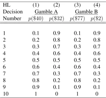
Holt and Laury (2002) pioneered the Multiple Price List (MPL) format, which is de-signed to elicit risk preferences. The format presents ten pairs of gambles. The participant then chooses her most-preferred gamble for each pair. The payoffs for the gambles are set so that Gamble B is more risky than Gamble A because the spread between payoffs is larger. The difference in expected value between Gamble A and Gamble B decreases as one moves down the table. Hence, the number of the gamble at which a person switches from the safe Gamble A column to the risky Gamble B column reveals her risk preferences. In Table 1, a risk-neutral participant would select the safe gamble in the first four decisions and the risky gamble in the last six decisions.
According to EUT, once an individual switches from preferring the safe column to preferring the risky column, it would be inconsistent for her to reverse back to the safe column in her choices. Although some studies design experiments so participants must be-have consistently, we do not impose the constraint of no reversals. Reversals in the price list indicate a reversals in risk preferences. Normative expected utility theory constrains risk preferences to be the same for all outcome and probability levels. Prospect theory allows for a reversal in risk preferences within the value function and the probability weighting function. For any agent who reverses his risk preferences, we can construct a pair of gam-bles in which a reversal of preferences would result in an irrational decision to give up an additional certain payoff.
Some evidence also suggests that individuals respond differently to hypothetical choices involving risk than they do in real-choice contexts [Battalio, Kagel, and Jiranyakul (1990); Laury (2002, 2005); and Taylor (2013)]. The real payoffs need to be sufficiently consequential to induce any difference in behavior. However, other studies find no sig-nificant difference in risk attitudes across settings [Beattie and Loomes (1997); Camerer and Hogarth (1999); Kang et al. (2011); and K¨uhberger, Schulte-Mecklenbeck, and Perner (2002)]. Therefore, we explicitly allow for a systematic difference in risk attitudes between real and hypothetical choices.
For each session of ten gambles that a participant completes, all ten choices are made in either a real or a hypothetical setting. Participants who considered gambles in the real setting were informed that they would make ten choices, one of which would be randomly selected to determine their payoff. Payoffs were relatively large–as high as $81. Those participants assigned to complete the hypothetical choices were informed that they would make ten choices, one of which would be randomly selected. They would then be shown how much their payoff would have been had the choice been real.
Procedure
The experiment was computer-based. It included a risk preferences task and a post-task section. The post-post-task section included a cognitive ability test and a survey that in-cluded demographic questions as well as questions about the individual’s preparation in math and economics. This questionnaire also inquired about whether participants had been distracted during the experiment, whether they were liquidity constrained, their education