Assessment of high-order finite volume methods on unstructured meshes for RANS solutions of aeronautical configurations

Antoniadis, Antonis F. and Tsoutsanis, Panagiotis and Drikakis, Dimitris

(2017) Assessment of high-order finite volume methods on unstructured

meshes for RANS solutions of aeronautical configurations. Computers

and Fluids, 146. pp. 86-104. ISSN 0045-7930 ,

http://dx.doi.org/10.1016/j.compfluid.2017.01.002

This version is available at

https://strathprints.strath.ac.uk/59947/

Strathprints is designed to allow users to access the research output of the University of Strathclyde. Unless otherwise explicitly stated on the manuscript, Copyright © and Moral Rights for the papers on this site are retained by the individual authors and/or other copyright owners. Please check the manuscript for details of any other licences that may have been applied. You may not engage in further distribution of the material for any profitmaking activities or any commercial gain. You may freely distribute both the url (https://strathprints.strath.ac.uk/) and the content of this paper for research or private study, educational, or not-for-profit purposes without prior permission or charge.

Any correspondence concerning this service should be sent to the Strathprints administrator:

[email protected]

Assessment of High-Order Finite Volume Methods on Unstructured Meshes

for RANS Solutions of Aeronautical Configurations.

Antonis F. Antoniadisa,∗_{, Panagiotis Tsoutsanis}a_{, Dimitris Drikakis}b a

Centre for Computational Engineering Sciences, Cranfield University, Cranfield MK43 0AL, United Kingdom

b

University of Strathclyde, Glasgow, G1 1XW, United Kingdom

Abstract

This paper is concerned with the application of k-exact finite volume methods for compressible Reynolds-Averaged Navier-Stokes computations of flows around aeronautical configurations including the NACA0012, RAE2822, MDA30P30N, ONERA-M6, CRM and DLR-F11. High-order spatial discretisation is obtained with the Weighted Essentially Non-Oscillatory and the Monotone-Upstream Central Scheme for Conserva-tion Laws methods on hybrid unstructured grids in two- and three- dimensions. Schemes of fifth, third and second order comprise the foundation of the analysis, with main findings suggesting that enhanced accuracy can be obtained with at least a third-order scheme. Steady state solutions are achieved with the implicit approximately factored Lower-Upper Symmetric Gauss-Seidel time advancing technique, conver-gence properties of each scheme are discussed. The Spalart-Allmaras turbulence model is employed where its discretisation with respect to the high-order framework is assessed. A low-Mach number treatment tech-nique is studied, where recovery of accuracy in low speed regions is exemplified. Results are compared with referenced data and discussed in terms of accuracy, grid dependence and computational budget.

1. Introduction

Reynolds-Averaged Navier-Stokes (RANS) methods are likely to remain the high-fidelity Computational Fluid Dynamics (CFD) modelling approach for the foreseeable future, with second-order discretisation schemes being the most common numerical methods in industrial CFD codes. Advanced turbulence sim-ulations such as Direct Numerical Simulation (DNS) and Large Eddy Simulation (LES) are prohibited in terms of computational cost for high Reynolds number flows around or inside complex geometries.

⇤

Corresponding author

Email addresses: [email protected](Antonis F. Antoniadis),[email protected]

Considerable research efforts have been spent into the development, implementation and assessment of high-order finite volume (FV) discretisation schemes for DNS and LES [1, 2]. High-order methods can achieve at least the same level of accuracy with second-order schemes but using coarser grids [3]. However, the enhanced efficiency is predominantly demonstrated for canonical cases and simple geometrical configurations. In the context of the present study concerning unstructured meshes around simple and complex aeronautical configurations, high-order schemes are referred to spatial discretisation of at least third-order accurate.

In the last decade, accuracy and efficiency considerations were the fundamental drivers for the devel-opment of high-order numerical schemes. Recent reviews on high-order methods were presented by Huynh et al. [4] and Wang et al. [5] highlighting the challenges and potential benefits of the methods compared with production codes. The vast majority of high-order schemes are based on the finite volume and the discontinuous Galerkin (DG) numerical frameworks. Other methods include the DG spectral element [6,7] and hybrid DG/FV methods [8–10]. High-order methods combined with solution adaptive techniques such as grid refinement and/or order enrichment demonstrate promising results on unstructured grids [11, 12]. The essentially non-oscillatory (ENO) and weighted-ENO (WENO) schemes were originally formulation for FV methods [13–15] for structured grids [16,17]. Furthermore, several research groups extended the original schemes to handle unstructured [18–22] as well as mixed-element unstructured grids [3,23–26], furthermore WENO methods are also utilised within the DG framework [27,28].

WENO schemes have been mainly used for inviscid, laminar and low Reynolds number flows [29, 30]. The grid requirements of high Reynolds number flows combined with low-quality highly skewed geometric elements poses a considerable robustness challenge for any high-order numerical method. For WENO schemes the grid sensitivity is mainly due to the inherited spatial extensiveness of the scheme, requiring large stencils for the reconstruction process. Furthermore, meshes with small neighbouring surface/volume ratio will benefit more as higher-order approximation of derivatives and gradient will be accurately estimated. The scheme is less sensitive to individual geometric quality metrics, as opposed to other framework, such as DG, where high-order grids would be required in order to explore their full potential of the method [31]. High-order spatial representation is a promising field, however for complex configurations often encounter in external aerodynamics, there is a limited number of tools available for accurate and efficient generation of high-order, curved meshes.

Numerical convergence and accuracy of CFD simulations can be further compromised by insufficient grid resolution, numerical dissipation and turbulence modelling issues. Furthermore, low Mach number effects can become important in near wall regions as well as in flow regions where vortical structures are

dominant [32,33]. Numerical methods designed for compressible flows should be assessed for their accuracy in these flow regions. Slow convergence rates and excessive numerical dissipation are often encountered in problems encompassing large changes in wave speeds. Local preconditioning methods [34,35] are popular techniques to address the stiffness of the resulting non-linear system. However, the computational expense can be excessive particularly for complex flow phenomena [36] such as unsteadiness, shock-wave-boundary layer interaction, transition and turbulence, which are often associated with buffet and flutter effects. A more compact technique with considerable smaller computational overhead was proposed by Thornber et al. [32] for block-structured grids and was investigated for a broad range of flows in [2]. The method was also employed in conjunction with implicit time-stepping in [37].

Implementation of high-order methods in conjunction with turbulence models poses additional chal-lenges with respect to robustness, accuracy and efficiency. High-order discretisation of the turbulence model transport equations can lead to non-physical (negative) eddy viscosity values, numerical artefacts and slow convergence rates [38]. Several researchers have documented irregularities attributed to the boundary layer edge-singularity inherited within wall-distance dependent turbulence models [39].

The development and implementation of the present high-order WENO and MUSCL schemes for un-structured grids has been presented for inviscid applications in [23]; for laminar, transitional and turbulent canonical and simple geometrical flows in the framework of Implicit Large Eddy Simulation (ILES) in [3] using an explicit time stepping technique. Although the utilisation of high-order methods makes more sense for long-time evolution of unsteady turbulent flow simulations, we explore the benefits that they can offer in the context of RANS simulations. Since in theory they should be able to provide smaller errors with respect to grid resolution, hence significant savings in terms of computational time. This paper assesses both the accuracy and efficiency of second- and third-order variants of the MUSCL scheme in conjunction with total variation diminishing (TVD) limiter functions as well as third- and fifth-order WENO schemes on mixed-element unstructured grids for subsonic and transonic flows around single aerofoils; multi-element aerofoils at high angle incidence; 3D wing; and aircraft configurations at cruise and landing conditions. The RANS computations have been carried out using an implicit lower-upper symmetric Gauss-Seidel (LU-SGS) method [40,41] and the one-equation Spalart-Allmaras (SA) turbulence model [42]. The paper is organized as follows. Section 2 is dedicated to the governing equations, Section 3 presents the high-order finite volume framework for unstructured meshes, the MUSCL and WENO methods, the flux treatment, the implicit time-stepping algorithm and the low-Mach number treatment method. The numerical results obtained for all the test-cases are presented in Sections 4. The conclusions drawn from the present study are outlined in

the last section.

2. Governing Equations

The compressible RANS equations with the one-equation Spalart-Allmaras (SA) turbulence model are written in conservative form as:

∂U₍x_{, t)}

∂t +∇(Fc(U)−Fv(U,∇U)) =S(U,∇U), (1) whereU_{is the vector of the conserved mean flow variables and the turbulence model variable, and}F_{c and} F_{v are the inviscid and viscous flux vectors, respectively:}

U_{= [ρ,ρu,ρv,ρw, E,ν]˜}T_, Fx c = ⇥ ρu,ρu2+p,ρuv,ρuw, u(E+p), uν˜⇤T , Fy_{c =}⇥ ρv,ρuv,ρv2+p,ρvw, v(E+p), vν˜⇤T , Fz c= ⇥ ρw,ρuw,ρvw,ρw2_{+p, w(E+p), wν˜}⇤T , Fx v =  0,τxx,τxy,τxz,Θ_x, 1 σ(νl+ ˜ν) ∂˜ν ∂x $T , Fy_{v =} 

0,τxy,τyy,τyz,Θ_y,1

σ(νl+ ˜ν) ∂ν˜ ∂y $T , Fz_{v =}  0,τxz,τyz,τzz,Θ_z, 1 σ(νl+ ˜ν) ∂˜ν ∂z $T , S₌ " 0,0,0,0,0, Cb1S˜˜ν+ 1 σCb2(∇ν)˜ 2 −Cw1fw ✓ ˜ ν d ◆2#T . (2)

In the above equations,ρis the density,u, v, w are the velocity components in x, y andzCartesian coordi-nates, respectively. Calorically perfect gas is assumed where the total energy per unit volume is calculated byE=p/(γ−1) + (1/2)ρ(u2_+v2_+w2_{), wherepis the pressure,γ= 1.4is the ratio of specific heats for air}

at normal atmospheric conditions;ν is the kinematic laminar viscosity andν˜is the SA turbulent viscosity working variable. The laminar viscosity is related to the temperature through the Sutherland law:

µl µ0 = ✓_T T0 ◆32 _T 0+S T+S, (3)

Sis the Sutherland temperature and the subscript0denotes a reference state for the corresponding variables. Unless otherwise stated, the reference values are taken at atmospheric conditions (sea level): dynamic viscosity µ0 = 1.7894×10−5kg/(ms); reference temperatures T0 = 288.16K; S = 110.4K; and Prandtl

numberP r= 0.72. Using the Boussinesq’s approximation the viscous stress tensorτij is defined by τij = (µl+µt) ✓ ∂u_i ∂x_j + ∂u_j ∂x_i − 2 3 ∂u_k ∂x_kδij ◆ , (4)

where µt is the eddy viscosity, δij is the Kronecker delta and the subscripts i, j, k refer to the Cartesian coordinate componentsx_{= (x, y, z). The work of viscous stresses and heat conduction,} Θ_{, is given by:}

Θ_{x=uτxx+vτxy+wτxz+} ✓ µ P r + µt P rt ◆ γ (γ−1) ∂T ∂x, Θ_{y=uτyx+vτyy+wτyz+}

✓ µ P r + µt P rt ◆ γ (γ−1) ∂T ∂y, Θ_{z=uτzz+vτzy+wτzz+} ✓ _µ P r + µt P rt ◆ γ (γ−1) ∂T ∂z. (5)

P rt is the turbulent Prandtl number; νt is the turbulent kinematic viscosity. The SA turbulence working variableν˜is related to eddy viscosityµtby:

µt=ρ˜νfv1, where fv1=

(ρ˜ν/µl)3

(ρ˜ν/µl)3_+C3

v1

and Cv1= 7.1. (6)

where the component of the source termS_{of equation (2) are given as:}

˜ S=Ω_+fv2 ν˜ κ2_d2, fv2= 1− (ρ˜ν/µl) 1 + (ρ˜ν/µl)fv1 , (7)

Ω_{is the vorticity magnitude and}

fw=g ✓_{1 +C} w36 g6_+C6 w3 ◆1/6

, where g=r+Cw2)r6−r* and r=min

✓ _˜ ν ˜ Sκ2_d2, rlim ◆ . (8)

The closure constants are:

Cb2= 0.622, Cw1= Cb1 κ2 + 1 +Cb2 σ , Cw2= 0.3, Cb1= 0.1355, Cw3= 2.0, σ= 2/3, κ= 0.41, rlim= 10, P rt= 0.9. (9) as given in [42]. 3. Numerical Framework

The discretisation in a domain Ω _{is achieved by combining conforming arbitrary shaped elements of} volume|Vi|. Integrating equation (1) over a mesh element using the finite volume formulation the following

ordinary differential equation is obtained dU_i dt =− 1 |Vi| Nf X l=1 Nqp X α=1 Fn_c,l₍U₍x_{α, t))}ωα|Al| + 1 |Vi| Nf X l=1 Nqp X α=1 Fn_v,l₍U₍x_{α, t),∇}U₍x_{α, t))ωα|Al|+}S_i, (10)

where U_{i is the volume averaged conserved variable vector,} S_{i is the volume averaged source term vector} within in a volume element i, Nf is the number of faces per element, Nqp is the number of quadrature points used for approximating the surface integrals. Figure 1 illustrates an example of quadrature point distribution on a aircraft surface mesh; the blue points located near the vertices correspond to quadrature weight smaller compared with the points located in the midsection coloured in red. |Al|is the surface area of the corresponding face, andα corresponds to different Gaussian integration points x_{α and weights} ωα over the face.

Figure 1: Close-up of the surface mesh and the corresponding quadrature points for a WENO third-order scheme, colour codes according to their corresponding weight value.

The weight and distribution of the quadrature points depend upon the order of the Gaussian quadrature rule employed, higher integration rule will result in enhanced interface flux approximation. The convective

and viscous flux tensors are defined as: Fn_c,l_=Fcx_nx+Fcy_ny+Fcz_nz, Fn_v,l_=Fx vnx+F y vny+F z vnz, (11)

where nx, ny and nz are the Cartesian components of the normal vector on the inter-element surface. The interface fluxes are computed from the reconstructed solution which is extrapolated at the interface. The solution is reconstructed from element-averaged data. The following section describe the methodology adopted for the reconstruction procedure.

3.1. Spatial Discretisation

The main objective of the reconstruction process is to build a high-order polynomialpi(x, y, z)of arbitrary orderr, for each considered elementVi that has the same average as a general quantityUi [43]. This can be formulated as U_i= 1 |Vi| ˆ Vi U_{(x, y, z)dV =} 1 |Vi| ˆ Vi pi(x, y, z)dV. (12)

The reconstruction method is based on the approach of [3,23], and only the key details are highlighted in this paper. The reconstruction is carried out in a transformed system of coordinates in order to minimize scaling effects that appear in stencils consisting of elements of different size as well as to improve the condition number of the system of equations [3,23,44]. The transformation is achieved by decomposing each element into tetrahedrals. Since a transformation based on shape functions of elements can fail when non-planar faces are encountered, this also applies to the quadrilateral faces, which need to be decomposed to triangular ones in order to accurately compute the normal vectors [3]. The reconstruction polynomial at the transformed elementV#

i is expanded over local polynomial basis functions labelled asφk(ξ,η,ζ), which are given by:

p(ξ,η,ζ) = K X k=0 akφk(ξ,η,ζ) =U0+ K X k=1 akφk(ξ,η,ζ), (13)

whereξ,η,ζare the coordinates in the reference system,akare the degrees of freedom and the upper index in the summation of expansion. Kis related to the order of the polynomialrbyK=1₆(r+ 1)(r+ 2)(r+ 3)−1. It must be stressed that the decomposition to tetrahedrals, is carried out to improve the condition of the reconstruction matrices only, rather than computing inter-element variables e.g. fluxes, since the use of prismatic or hexahedral elements for the boundary layer region is beneficial for computing the gradients with high-accuracy. For computing the degrees of freedomak, a minimum ofK elements is required in the stencil in addition to the target element. Using the minimum possible number of elements in the stencil, M ≡K, may produce ill-conditioned systems, hence usingM = 2·Kimproves the robustness of the method

as described in [23,44]. A linear least-square method is adopted to enable the system of equations of (13) for the unknown degrees of freedomak. The final form of the linear system is solve with the QR decomposition algorithm. Discontinuous solutions are often encounter in external aerodynamics, thus limiting functions are essential for maintaining numerical stability and suppress any spurious oscillations. Two approaches are assessed in this work the MUSCL and the WENO schemes.

3.1.1. MUSCL

The MUSCL scheme employed in this work is based on the Barth and Jespersen slope limiter [45]. The design of the scheme requires the minimum and maximum values in the stencil’s neighbourhood, i.e.,

Umin

i =min(Ui, Ul)andUimax=max(Ui, Ul), wherel= 1, ..L;Lis the total number neighbours of element

i. The gradient of a general quantity is defined as∇Uiand is an approximation of the solution gradient inside the element i. The gradient is computed during the reconstruction process by incorporating information from the entire central stencil. The scheme is written as

Uiα=Uic+φi∇Ui·xα, (14)

where Uc

i is the value for the general quantity at the element centroid and xα are the coordinates of the quadrature point. The limiter seeks the minimum value of the slope limiter for all the quadrature points that satisfy conditions: φi = min(φi,m1,φi,m2, ...φi,M). Then, the limiting function is applied, composed by three different states according to the difference of the reconstructed value at the quadrature points of the considered elementU(i,α), the minimum and maximum values from the neighboursUl, and the element centre valueUi, yielding:

φi,α= 8 > > > > > < > > > > > : min ✓ 1,U max i −Ui Ui,α−Ui ◆ , ifUi,α−Ui >0 min ✓ 1,U min i −Ui Ui,α−Ui ◆ , ifUi,α−Ui <0 1, ifUi,α−Ui= 0. (15) 3.1.2. WENO

WENO schemes use a non-linear combination of various reconstruction polynomials, where each poly-nomial is weighted according to the smoothness of its solution. The polypoly-nomials are given by

pweno i = ms X m=1 ωmpm(ξ,η,ζ), (16)

where ms is the total number of WENO stencils. Substituting back to equation (13) for pm(ξ,η,ζ), we obtain the following expression

pm(ξ,η,ζ) = K

X

m=0

a(_km)φk(ξ,η,ζ). (17)

Using the condition that the sum of all weights is unity, yields pwenoi =U0+ K X k=1 ms X m=0 ωmamk ! φk(ξ,η,ζ)≡U₀₊ K X k=1 ˜ akφk(ξ,η,ζ), (18)

where˜ak are the reconstructed degrees of freedom; and the non-linear weightωm as ωm= _mωm˜_s P m=0 ˜ ωm where ωm˜ = λm (0+Im)b. (19)

The smoothness indicator is given by

Im= X 1≤|β|≤r ˆ ˜ Ei ) Dβ_pm(ξ,η,ζ)*2 (dξ, dη, dζ), (20)

where β is a multi-index, r is the polynomial’s order, λm is the linear weight, and D is the derivative operator. The smoothness indicator is a quadratic function of the degrees of freedom (am

k) and can be expressed as a universal mesh-independent oscillation indicator matrix.

The various reconstruction polynomials arise from different sets of stencils that satisfy some geometrical conditions. The reader is referred to [3,23, 44], and references therein, for a comprehensive explanation of the different set of geometrical conditions and WENO characteristic reconstruction.

Additionally for the MUSCL and WENO schemes for ensuring that the pressure and density remain positive through the reconstruction the positivity condition of [13] is used where the reconstructed values of density and pressure for each Gaussian quadrature points(α)must satisfy the following condition:

|ρiα−ρi|<0.8ρi and |piα−pi|<0.8pi. (21) If the condition (21) is not satisfied for all Gaussian quadrature points then the reconstruction order for the considered element is reduced by one order until the condition is satisfied.

3.2. Fluxes Approximation

Having reconstructed the element-averaged solutions, the interface fluxes can be evaluated. For the convective fluxes the Riemann problem is solved with the approximate Harten-Lax-van Leer-Contact (HLLC) solver as proposed in [46]. The HLLC solver is also employed for the convective part of the turbulence transport equation when a higher than first-order discretisation of the turbulence variable is adopted. The

HLLC flux function is given as: ˆ FHLLC 8 > > > > > > > < > > > > > > > : ˆ F−_{, if0} ≤S−_, ˆ F∗− _{= ˆF}−_+S−⇣_Wˆ∗− −Wˆ−⌘_{, ifS}− ≤0≤S∗_, ˆ F∗+ _{= ˆF}+_+S+⇣_Wˆ∗+ −Wˆ+⌘_{, ifS}∗ ≤0≤S+_, ˆ F+_{, if0} ≥S+_, (22) where ˆ W∗±_=ρ± ✓ S± −u± S±_−S∗ ◆ 2 6 6 6 6 6 6 6 6 6 6 6 6 6 6 4 1 S∗ v± w± E± ρ± (S ∗ −u±₎ ✓ S∗₊ p± ρ±) S±−u±* ◆ ˜ ν ρ± 3 7 7 7 7 7 7 7 7 7 7 7 7 7 7 5 . (23) ˆ

W∗± _{is computed either for the considered element “}

−”, or for its neighbour “+” and the wave speeds +S−_,+S+_{, S}∗ _{are approximated by an adaptive iterative procedure as detailed in [46].}

The discretisation of the convective turbulence flux term has significant impact on the amount of artificial dissipation produced by the turbulence model. Disproportional amounts of eddy viscosity are introduced when there is a severe mismatch between the discretisation of the mean flow and turbulence model equations. Mispredictions of eddy viscosity production can lead to very small or negative values. Several numerical experiments were performed in order to establish the most stable and accurate methodology for the discreti-sation of the turbulence model terms, including the convective component, the turbulence model variable gradients and source terms which are depended upon the velocity, turbulence model gradients. For second-order mean flow discretisation, a first-second-order upwind flux is employed for the turbulence model convective term and the second-order scheme for all gradients. The convective turbulent flux Fˆ˜ν

c for a second-order scheme is computed as ˆ Fν˜ c = 1 2 ⇥ N) (˜ν)−_{+ (˜ν)}+* −|N |) (˜ν)+ −(˜ν)−*⇤ , (24)

where (ν)− _{and (ν)}+ _{are the element-centred values of the turbulent eddy viscosity for the considered}

element and its direct side neighbour, respectively, withN defined as

N =1 2 ⇥ nx ) u−_+u+* +ny ) v−_+v+* +nz ) w−_+w+*⇤ , (25)

For high-order mean flow discretisation it was found that the most stable method with accurate solutions, is to treat the turbulence convective term through the Riemann solver as shown in equation (23). The turbulence model variable is reconstructed according to the high-order spatial scheme of the mean flow equations either with a MUSCL or WENO approach whereas the gradients are estimated with the same approach as viscous terms. For the evaluation of the viscous fluxes the extrapolated interface variables Ui,a± and their unlimited gradients ∇Ui,a± from the k-exact least square reconstruction of equation (12) are averaged from two discontinuous states as detailed in [3,47]. Although, other methods for the evaluation of the diffusive fluxes such as the one of the generalised Riemann problem of Gassner et al. [48], or the diffusive flux of direct DG [49, 50] can be applied, the k-order accurate flux is implemented as it easily obtained through element centred reconstructions and has been applied for various flows problems [47,51,52].

This k-exact reconstruction flux approximation has been previously assessed by Ivan and Groth [47] and it is not susceptible to odd-even decoupling, however the discrete maximum principle is not satisfied and is influenced by the mesh quality, which agrees with the rule that for finite volume discretisation methods, accuracy and positivity are conflicting properties. Therefore, for stability purposes, and when dealing with meshes consisting of non-planar quadrilateral faces, hence poor quality hexahedral, prisms and pyramids, the least square reconstruction can introduce severe errors in the computation of the viscous flux gradients. As it has been reported by Diskin et al [53], where extensive tests have been performed for different grid topologies with high aspect ratio and skewness elements, the Green-Gauss formulation for computing the viscous terms is much more robust and less sensitive to the quality of the grid element.

In the presence low radius curvature (e.g. leading edge of a wing) highly skewed elements can introduce large errors when computing their gradients with a least square reconstruction of high-order polynomial. Therefore, for each element that has an aspect-ratio greater than a threshold value ≈100, we utilise the Green-Gauss formulation as described in [3], otherwise the least square reconstruction procedure for the gradients is employed. This condition of gradient approximation is only applicable to the gradients of the viscous terms. In the convective terms, the least square reconstruction is used both with the MUSCL and WENO schemes.

3.3. Low-Mach Number Treatment Modification

A low-Mach number modification is employed in the present study for subsonic flows and it follows the previous work of Thornber et al. [32], where the left and right state of the reconstructed velocities,normal to the interface are modified in a linear way with respect to the local Mach number. In the case of the local

speed approaches to zero the arithmetic mean of them is modified in the following manner: u∗ L = (1 +ζ)uL+ (1−ζ)uR 2 , u ∗ R= (1 +ζ)uR+ (1−ζ)uL 2 , (26)

with the functionζbeing equal toζ=min(1, max(ML, MR)). The Mach number for the left and right states are calculated based on the velocity magnitude of all the velocity components independent of the normal direction in which the flux is computed. This modification is different in nature from a preconditioning step used for changing the flow variables, since our main motivation is not to relax the restriction in terms of the time-step size, but rather to increase the resolution at low speed regions, where this modification has demonstrated increased resolution and accuracy for a wide-range of flow problems [1,2,32, 33,54], can be utilised with any Riemann solver and without computational overheads.

3.4. Time discretisation

Convergence to steady state solution are obtained with the lower-upper symmetric Gauss-Seidel (LU-SGS) implicit time integration method in conjunction with local time stepping algorithm. The LU scheme was introduced by Jameson [55] and it is extensively used for high-Reynolds number flows on unstruc-tured grids [56–61] in various formulations including WENO and Spectral schemes. Although, alternative implicit-time stepping methods are introduced for unstructured grids e.g. the Newton-Krylov GMRES implementations [62], the present time advancement scheme is considered to be robust with efficient par-allelisation and low computational cost. The LU-SGS scheme with an approximate first-order Jacobian is considered. Equation (10) can be rewritten in the following semi-discrete form

dU_i

dt =Ri, (27)

where R_{i is the right-hand side residual, which should converge to the machine precision. Employing a} first-order backward Euler implicit time stepping scheme, equation (27) takes the following form

dUn_i dt = Un+1 i −Uni dt =R n+1 i . (28)

Linearising in time, equation (28) gives

dUn_i dt =R n i + ∂Rn_i ∂U , (29)

whereR_{i should be equal to zero, hence equation (29) becomes}

✓_I dt − ∂Rn i ∂U ◆ dU_{i =}Rn i. (30)

The solution at each elementiis updated asUn+1

i =Uni +dUi, whereIstands for the identity matrix. The term ∂Rni

∂U is the Jacobian matrix and contains the linearisation of the inviscid and viscous flux vectors as well as the source terms. For obtaining the quadratic convergence properties of the Newton’s method, the linearisation of the numerical flux function must be exact. However the formulation of the exact Jacobian matrices for high-order non-linear schemes such as WENO methods, require excessive memory storage [41, 63]. Since we are only interested in steady state solutions and in order to simplify the linearisation of the Jacobian, a first-order approximation of the numerical fluxes is employed, since the matrix of ∂Rni ∂U is identical to the graph of the corresponding unstructured grid. The numerical flux is estimated with the Rusanov flux function given as

R_i(U_i,U_{j, nij) =}1 2 )_Fnij c,v(Ui,∇Ui) +F nij c,v(Uj,∇Uj)*− 1 2|λ ij c +λijv|(Uj−Ui), (31) with the maximum convective and viscous eigenvalue written respectively

λijc =|Vij·nij|+aij, λijv =

µij ρij|xj−xi|

, (32)

where n_{ij is the normal vector to the element interface,} V_{ij is the velocity vector and aij is the speed} of sound. The viscous eigenvalue is approximated by the viscous spectral radius xj −xi of the element barycenter. Linearising the Rusanov flux of equation (31) gives the diagonal and off-diagonal components respectively: ∂R_i ∂U_i = 1 2 ✓ ∂F_c,v ∂U_i +|λ ij c +λijv|I ◆ , ∂R_i ∂U_j = 1 2 ✓ ∂F_c,v ∂U_j −|λ ij c +λijv|I ◆ . (33)

Due to these approximations, the quadratic convergence of the Newton’s method will not be achieved due to the discrepancy in the resolution of the right- and left-hand sides of equation (30). The resulting linear system of the form AX = B of equation (30), following the implementation of [58], is solved by a two step approach, consisting of two sweeps; the forward and backward sweeps are given by the following two equations upper and lower part, respectively:

WhereU∗ _{is the intermediate state, the upper, lower and diagonal components of the system of equations} are written as U = 1 2 ✓ ∂F_c,v ∂U_i −|λ ij c +λijv|I ◆ , L= 1 2 ✓ −∂Fc,v ∂U_j −|λ ij c +λijv|I ◆ , D= I dt+ Nf X l=1 1 2 ✓ ∂F_c,v ∂U_i +|λ ij c +λijv|I ◆ − ∂S ∂U. (35)

The implicit scheme has small computational cost per iteration and the only storage requirements arise from the diagonal of the equation above. The diagonal elements of the matrix must be stored and inverted directly and the off-diagonal ones are computed at every stage. Hence, the diagonal elements used in the present study are scalars multiplied by the identity matrix and the off-diagonals are computed according to equation (33). The number of sweeps per Newton iteration is set to 5 in the present study, based on the findings of various approaches using the LU-SGS schemes for similar flow problems [56–61]. The source termS is differentiated with respect to the turbulence model variable only, in order to keep the diagonal dominance of the system matrix, and the source term Jacobian is restricted to be positive as suggested by [42], hence dS dν˜ =Cb1S˜+ 1 σCb22 (∇ν˜)−2Cw1fw ✓_ν˜ d2 ◆ ≤0. (36)

Finally, the boundary conditions are also treated implicitly according to Batten et al. [63].

4. Results and Discussion

Computations are performed for three two-dimensional and three three-dimensional external aerody-namic flows of aeronautical configurations. The MUSCL second- and third-order schemes and the WENO third- and fifth-order schemes are employed, henceforth labelled as M2, M3, W3 and W5, respectively. The MUSCL schemes of higher-order of accuracy are not pursued since due to their non-differentiable nature of the limiters they can not achieve higher-order of accuracy. The W3 scheme has a desirable balance between accuracy and computational cost, whereas the W5 is significantly more expensive. High-order discretisation of turbulence model variable in a coupled fashion is extensively assessed and presented for some represen-tative case. The low-Mach number treatment technique is investigated and the findings are presented with main focus on flows with regions of low velocity. Three types of boundary conditions are implemented, no-slip wall for all body surfaces, characteristics based far-field boundary conditions and where appropriate symmetry conditions. The flow cases are presented in an escalating level in terms of difficulty, complexity

and overall computational effort. Grid convergence study is performed for all cases excluding the flow over the DLR-F11 aircraft configuration due to computational budgets available. Grid refinement strategy fol-lows the simple rule of halving the element size on the wall surface; the strategy is applied in regions of interest i.e. near boundary layers, shocks and wakes. Computations are performed without wall-functions thus y+ values are kept to unity.

4.1. NACA-0012

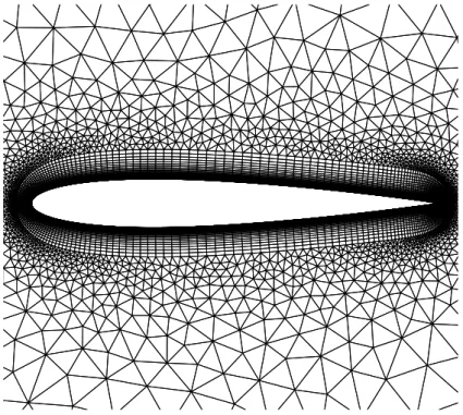
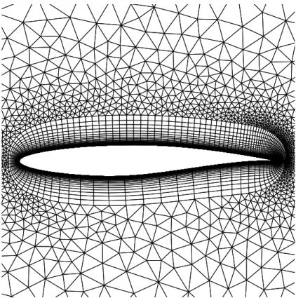
The first case concerns the subsonic turbulent flow around the symmetric NACA-0012 aerofoil at zero degree incidence. Freestream conditions correspond a Mach number ofM∞= 0.3, angle of attack ofα= 0◦ and a Reynolds number ofRec= 1.85×106based on the aerofoil chord length. Five grids are generated, the grid statistics are shown in table1. A hyperbolic method is employed for the inflation of the quadrilateral layer with a constant growth rate of 1.1; figure 2 shows a close-up of the coarse grid topology. The aim of this test case is to evaluate the benefit of high-order reconstruction methodology for RANS solutions on fully attached flow over symmetric aerofoils.

Figure 2: Close-up of the coarse grid for the NACA-0012 aerofoil.

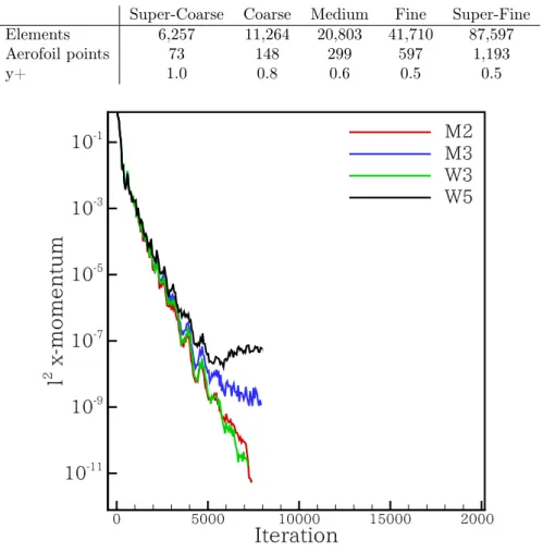
With respect to convergence properties the solutions of order smaller than fifth exhibit a residual drop of at least eight orders of magnitude, where the fifth order solution suggests a plateau at10−7_{, this is also}

Table 1: Grid properties for the NACA-0012 test case.

Super-Coarse Coarse Medium Fine Super-Fine

Elements 6,257 11,264 20,803 41,710 87,597

Aerofoil points 73 148 299 597 1,193

y+ 1.0 0.8 0.6 0.5 0.5

Figure 3: Residuals forl2

norms of x-momentum for the subsonic flow over the NACA-0012 aerofoil on the fine grid (M1= 0.3

α= 0◦andRec= 1.85×106).

are depicted in figure 3 where the l2 _{norms of x-momentum (ρu) on the super-fine grid are plotted for}

the MUSCL and WENO solutions of second and third, and third and fifth order, respectively. It is worth mentioning that the convergence rate is similar for all spatial schemes including the conserved variables and turbulence parameter (ρ,ρu,ρv, E, µ) up until5,000iterations and no considerable grid dependence is observed with respect to either the speed or the convergence levels.

In terms of accuracy, the pressure coefficient (Cp) estimates are shown in figure4and compared with the experimental data obtained from the AGARD report [64]. This case is characterised by a smooth attached flow throughout the surface of the aerofoil, which is also predicted by the computed solutions, leading to good agreement with the experiment. There are no apparent differences in theCp profiles for all numerical schemes on the fine grid, however there are variations in the drag prediction.

Figure 4: Pressure coefficient (Cp) on the fine grid for the NACA-0012 case compared with experiment data [64] (M1= 0.3

α= 0◦andRec= 1.85×106).

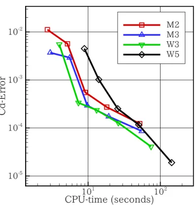
the wall-clock time. The relative drag error is computed based on an additional refinement M2 solution, where the indicative wall clock time is based on the computations performed on a intel-i7 3820 four core processor. Each line corresponds to one numerical scheme for the five grid refinements, starting from the left hand side with the coarse one. Only WENO predictions can reach lower than 10−_{4 error levels for} the given grids. W5 solutions demonstrate higher error for the same spatial refinement compared with the W3, this may be attributed to the higher grid quality requirements of the stencil construction in terms of smoothness and isotropy for the fifth order scheme compared with the third-order one. Additionally, the imbalance in the resolution between the left and right hand side of the implicit time-stepping due to the first-order Jacobian approximation could also be responsible for this behaviour. It has to be noted, that for the super-coarse and coarse grids the average aspect ratio in the vicinity of the aerofoil surface is around 5,000.

4.2. RAE-2822

The shock capturing capabilities of the numerical framework are assessed with the two-dimensional transonic flow around the RAE-2822 supercritical aerofoil. The freestream conditions are based on the wind tunnel measurements performed in 1979 and presented in the technical report by Cook et al. [65]. Case 6

Figure 5: Relative drag error against wall-clock time in seconds on an i7-3820 processor for the NACA-0012 case (M1= 0.3

α= 0◦andRec= 1.85×106).

is investigated where the wind tunnel freestream conditions correspond to a Mach number ofM∞= 0.725, an angle of incidence ofα= 2.92◦ _{and Reynolds number based on the aerofoil chord of Re}

c = 6.5×106. Several modifications on the Mach number and angle of attack have been proposed in order to account for wall interference. The corrected Mach number of M∞ = 0.729, angle of attack ofα= 2.31◦ and with the same Reynolds number are adopted for the current analysis as performed also in [66].

The outer boundary is positioned approximately 100 chord lengths away from the aerofoil to minimize any artificial reflections from the outer boundary conditions. The flow is characterised by a normal shock on the upper surface of the aerofoil interacting with the boundary layer, which considerably thickens downstream up to the end of the trailing edge. To account for the shock-wave boundary layer interaction on the suction side and benefit of the flexibility of unstructured grids a non-uniform distribution of points is set for the upper and lower part of the aerofoil. Three hybrid unstructured grids are generated their details are tabulated in table2, the meshes are generated based on the o-grid strategy, the coarse grid is shown in figure6.

High-order discretisation of turbulence model poses robustness and accuracy challenges for the RANS computations. Negative values of eddy viscosity in the vicinity of the boundary layer edge as well as non-physical oscillations are often encountered in high Reynolds number flows with high-order approximations

Figure 6: Coarse grid for the RAE-2822 case. Table 2: Grid properties for the RAE-2822 test case.

Coarse Medium Fine

Elements 10,714 23,852 51,294

Upper surface points 85 170 341

Lower surface points 45 90 188

y+ 1.0 0.8 0.6

particularly for under-resolved grids [38,67,68]. The effect of discretisation of the turbulence parameter for high-order reconstruction is presented for this case in terms of accuracy and convergence. Figure7 depicts the residual histories on the fine grid for the second, third and fifth order schemes, where the coupled (COU) approach refers to a discretisation of the turbulence parameter according to the type (WENO or MUSCL) and order of the mean flow variable approximation, whereas the decoupled refers to a discretisation of the turbulence parameter according to a first order upwind method, shown in equation (24). The residual histories suggest that for the third and fifth order coupled results, a lower drop than the decoupled ones is achieved. However, this is not the case for the second order solution, which could be attributed to the non-differentiable nature of the slope limiter used for the turbulence model variable that in turn influences the mean flow residuals. The two discretisation approaches differ also on the level of eddy viscosity production,

Figure 7: Residual histories ofl2

norm for total energy for the RAE-2822 aerofoil (M1= 0.729,α= 2.31◦andRec= 6.5×106).

particularly for the higher-order solutions, this is illustrated in figure8 for the WENO third order solution on the fine grid.

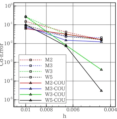
In terms of accuracy the coupled approach for higher than third order discretisation is shown in figure

9 where the relative drag coefficient is plotted against grid refinement defined as h= 1/√Elements. The benefit of discretising the turbulence parameter according to the mean flow equation method is amplified with higher grid resolution for the WENO method, where the MUSCL type solution suggest small differences between the coupled and decoupled approach. This effect is also demonstrated in figure 10, where the coefficient of pressure on the coarse grid is compared against the fine fifth order solution and the experimental data of Cook et al. [65]. Henceforth all solutions presented in this work correspond to the coupled method for higher than second order schemes and only for the second order solutions a decoupled manner is adopted including the NACA-0012 case.

4.3. MDA 30P-30N

Flow phenomena around high-lift devices are considered challenging for numerical methods and turbu-lence model discretisation; deployed slat and flap at high angles of attack in combination with low speed, potential unsteady flow regime, flow separation, laminar/turbulent transition, interaction of aerofoil/wing

Figure 8: Eddy viscosity production for the coupled and decoupled approaches on the WENO third order fine grid for the RAE-2822 aerofoil (M1= 0.729,α= 2.31◦andRec= 6.5×106).

elements, streamline curvature, wake in pressure gradient are some of the them. A well established case for assessing the performance and accuracy of the developed numerical framework for flow over high-lift devices is the McDonnell Douglas three-element configuration at 30P-30N or simply MDA 30P-30N. The freestream conditions correspond to a Mach number of M∞ = 0.2, an angle of incidence of α = 16◦ and Reynolds number based on the reference aerofoil chord length ofRec = 9×106. The flow around this configuration has been previously studied experimentally by Spaid [69] and by Rumsey et al [70], where 3D effects are analysed including CFD simulations, further CFD work is presented in the following papers [71–74].

Three hybrid unstructured grids are generated, labelled as coarse, medium and fine the grid properties are presented in table3 where the grid topology is visualised in figure11for the medium grid. The grid is locally refined around the aerofoil elements and the wake.

The flow over the high lift aerofoil is characterised by several low speed regions i.e. at the lower surface of the slat and inside the slot with the sharp corner cove. Compressible solvers inherently struggle with low

Figure 9: Relative drag coefficient error for different grid for the RAE-2822 aerofoil (M1 = 0.729,α = 2.31◦ and Rec =

6.5×106).

Table 3: Grid proprerties for the MDA-30P-30N aerofoil.

Coarse Medium Fine

Elements 34,184 74,902 192,845

Slat points 90 147 284

Main element points 203 372 667

Flap points 85 140 265

y+ 1.0 0.8 0.6

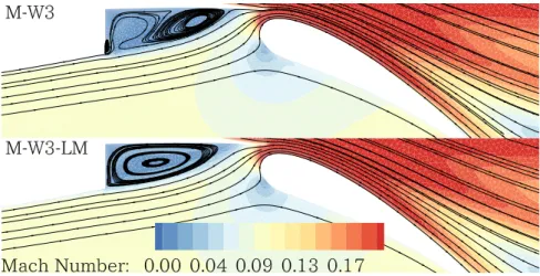
speed flow regions, due to the stiffness of the system of equations, leading to slow convergence rates and impaired accuracy. To surpass the accuracy challenge the low-Mach number treatment method presented in the previous section is investigated. Simulations are performed with the second and third order MUSCL scheme as well as with the third and fifth order WENO, with and without the low-Mach number (LM) treatment. The benefit of the low-Mach number treatment in terms of flow structures is most evident in low speed regions, predicting an accurate representation of the flow, illustrated in figure13where Mach number contours are plotted, overlaid with streamlines on the medium grid W3 solutions. The LM treatment effect is also mirrored on the increased eddy viscosity production near low velocity regions, depicted in figure12

Figure 10: Coefficient of pressure (Cp) variations for the coupled and decoupled approaches on the RAE-2822 aerofoil compared with the experimental data [65] (M1= 0.729,α= 2.31

◦

andRec= 6.5×106).

Figure 11: Medium grid for the MDA 30P-30N multi-element aerofoil

of eddy viscosity are observed.

Convergence rates for higher order schemes with low-Mach number treatment don’t exhibit particular improvement, however for second order not only the rate of convergence is faster but also the plateau is reached much lower. This trend is amplified for the residuals of the turbulence working variable as exemplified in figure14, where thel2 _{norms for the SA turbulence working variableν and energy are plotted against}

the total number of iterations for the medium grid second order solutions.

Coefficients of drag and lift are plotted in figures15(a) and (b) respectively for all schemes against grid refinement. All solutions demonstrate monotone trends towards a grid independent solution for both drag

Figure 12: Contours of eddy viscosity (µt) for the medium grid W3 solutions, MDA 30P-30N aerofoil (M1= 0.2,α= 16 ◦

and

Rec= 9×106).

Figure 13: Contours of Mach number and streamlines for the medium grid W3 solutions, MDA 30P-30N aerofoil (M1= 0.2,

α= 16◦andRec= 9×106).

and lift except third and fifth order WENO without low-Mach number treatment on the fine grid. Higher resolution either by grid or polynomial order results to an increased lift and a decreased drag. The predicted Cl and Cd values agree well with values reported by other works [74] as well with the experimental lift coefficient of 4.1 (+/- 0.05) [70]. The advantage of the low-Mach number treatment is demonstrated for the two outliers mentioned earlier W3 and W5 on the fine grid, without the treatment the solution divergences and oscillations are observed in the wake which is due to the inherent unsteadiness of the solution at the flap wake, that the coupling of the turbulence model variable is not sufficient to produce the levels of eddy viscosity to supress these oscillations. This is again demonstrated when comparing the coefficient of pressure on the three elements with the M3 and W3 schemes against the experimental values in figure16.

Figure 14: Residuals of turbulent variableνand total energy for the second order solutions with and without low-Mach number

treatment, MDA 30P-30N aerofoil (M1= 0.2,α= 16 ◦

andRec= 9×106).

(a) Cl (b) Cd

Figure 16: Coefficient of pressure for the coarse grid M3 and W3 solutions compared with experimental data [70], MDA 30P-30N aerofoil (M1= 0.2,α= 16◦andRec= 9×106).

4.4. ONERA-M6

The three dimensional solver capabilities are assessed with the turbulent transonic flow around the ONERA-M6 wing; freestream conditions are set: Mach number of M∞ = 0.84, an angle of attack of

a = 3.06◦ _{and a Reynolds number of Re}

c = 11.72×106 based on the mean aerodynamic chord. The ONERA-M6 is a swept-span wing, with no twist and symmetrical aerofoil section and a rounded tip. Wing tunnel measurements were conducted by Schmitt and Charpin [75] and pressure data are publicly available with an error margin for Cp of±0.02. The transonic flow is characterised by a pair ofλ-structured shocks on the upper surface of the wing where they coincide towards the wing tip.

(a) Coarse (b) Medium

Figure 17: Grid topologies for the ONERA M6 wing.

(a)y/b= 0.2 (b)y/b= 0.44

(c)y/b= 0.90 (d)y/b= 0.95

Figure 18: Coefficient of pressure for the W3 and W5 solutions at four spanwise stations compared with experimental data [75] (M1= 0.84,α= 3.06

◦

andRec= 11.72×106).

projected normal to the wall to generate the prismatic layer followed by tetrahedra for the outer far field. Grid statistics are presented in table4, the medium and fine grid are locally refined near the shock location as presented in figures17.

(a) Cl (b) Cd Figure 19: Lift and drag coefficients against grid points for the ONERA M6 wing (M1= 0.84,α= 3.06

◦

andRec= 11.72×106).

Table 4: Grid properties for the ONERA M6 wing.

Coarse Medium Fine

Elements 1,170,073 1,739,464 3,557,505

Triangles on wing’s surface 38,389 43,720 69,692

y+ 1.0 1.0 0.8

when compared with the experimental data [75], this can be depicted from the coefficient of pressure in figures18, where the Cp is plotted at four spanwise sections where solutions of the WENO third and fifth order schemes are plotted for the three grid refinements. By either refining the grid or increasing the order of the scheme the predicted lift is increased and the drag decreased as shown in figure 18, where the Cl and Cd is plotted against grid size for all schemes. It is worth noting that higher order schemes (M3,W3 and W5) seem to converge within a narrower Cl and Cd range particularly for the finer grid resolutions, demonstrating that they reach grid-independent solutions faster than second order schemes.

4.5. CRM

This test case concerns the transonic flow over an aircraft configuration, the NASA Common Research Model (CRM) at cruise flight conditions. Drag prediction of the CRM model has been the main objective for the 4th_{, 5}th _{and 6}th _{drag prediction workshops [76,77].}

Case 1a from the 4th _{workshop is considered for the current analysis, the CRM configuration includes} wing, body and horizontal stabilizer. The flow is computed at a constant lift of Cl = 0.5 with error of

Figure 20: Grid configurations for the transonic flow over the CRM model.

Figure 21: Continuity residuals and lift histories for the W3 solutions, CRM configuration (M1 = 0.85, Cl = 0.5 and

Rec= 5.0×106 ).

±0.001. Wind tunnel measurement are carried out at the National Transonic Facility (NTF) at NASA Langley. The NTF data are publicly available which include drag polar, the corresponding coefficient of lift and main wing pressure measurements at several spanwise stations. The freestream conditions correspond to a Mach number ofM = 0.85with a Reynolds number of5×106_{based on the reference chord length. Two}

where the medium represents standard engineering practices; the grid surface distribution is shown in figure

20. The grid is locally refinement on the main wing and horizontal stabilizer.

The computations are initialised with an educated guess on the angle of attack, after the simulation has converged the angle is extrapolated for the first run and then linearly interpolated until the target lift is reached within the lift threshold. An example of the computations procedure is shown in figure21where the l2 _{norm of continuity and the Cl histories are plotted. A residual drop of at least ten orders of magnitude is}

achieved for both grids for the W3 scheme. According to the findings of the two dimensional transonic flow case RAE-2822 presented in the previous sections, the results with the third order MUSCL reconstruction did not demonstrate noticeable benefits compared with the second order solutions, in terms of shock location and forces predictions. Therefore, for the present transonic case the main objective is to assess the WENO third and fifth order methods and compare them with the industry workhorse-second order upwind solution as well with reference experimental and CFD data.

The coefficient of pressure on the CRM configuration is shown in figure 22 and at two representative spanwise stations on the main wing in figure23. The third and fifth order profiles are plotted against the chord-wise length and compared with the NTF pressure measurements [76]. The presence of the shock on the wing’s suction side is evident for both stations near the wing’s mid-spanwise location. Grid refinement suggests smaller discrepancies with respect to the shock position (η= 0.60) compared with the experiment regardless the scheme.

Table 5: Computed Drag for all schemes and grids compared with the average CFD and experimental values [76].

Elements(106_{) a C} d ∆Cd (counts) C-M2 3.5 2.395 0.03227 47.6 C-W3 3.5 2.295 0.02962 21.11 C-W5 3.5 2.360 0.02942 19.06 M-M2 11.0 2.210 0.02810 5.89 M-W3 11.0 2.236 0.02742 0.93 M-W5 11.0 2.264 0.02716 3.49 DPW-CFD - 2.340 0.02701 5 DPW-NTF - 3.020 0.02751

-Forces predictions are summarised in table 6, where for each run the angle of attack for constant lift, the predicted drag coefficient and the error ∆_{Cd in terms of drag counts with respect to the experiment} [76] are presented. The first apparent observation for the predicted drag is that the standard deviation σ for the fine grid is at least three times smaller than for the one on the coarse grid. Moreover, second order drag estimates, irrespective of the grid, have at least twice greater σ compared with WENO predictions. Both WENO solutions on the fine grid suggest lower ∆_{Cd than 5 drag counts representing the averaged}

CFD predictions of the workshop data [76]. Considering the additional computational cost of the fifth order scheme and the associated gains in terms of accuracy for the subject test-case, the W3 scheme represents a more suitable method with a favourable balance between cost and accuracy for these type of configurations.

Figure 22: Coefficient of pressure on the medium grid W3 solutions, CRM configuration (M1 = 0.85,Cl= 0.5and Rec =

5.0×106).

(a)η= 0.50 (b)η= 0.60

Figure 23: Coefficient of pressure at two spanwise stations (η) on the main wing compared with the wind tunnel measurement

[76], CRM configuration (M1= 0.85,C_l= 0.5andRec= 5.0×106).

4.6. DLR-F11

Following the series of computations with the two dimensional high-lift device (MDA 30P-30N), the flow around the DLR-F11, a full aircraft configuration at landing conditions is computed. According to the

Table 6: Coefficients of lift and drag compared with experimental data [78] and wall-clock time (hours) on 64 cores of Intel E5-2660 CPUs, DLR-F11 configuration.

Time CL CD CL/CD Experiment - 2.6796 0.2755 9.7278 M2 22.1 2.5514 0.3002 8.4984 M2-LM 22.1 2.6572 0.3043 8.7328 M3 26.5 2.5822 0.2993 8.6276 M3-LM 26.5 2.6842 0.3044 8.8171 W3 41.9 2.6197 0.3016 8.6857 W3-LM 41.9 2.6977 0.3047 8.8522

findings from the CRM case, the W3 method was found to be the best compromise in terms of resources/cost, henceforth, the second and third order schemes would be employed for the DLR-F11 flow problem. In addition, the effect of the low-Mach number treatment technique is assessed. The increased complexity of the configuration lies with the flow conditions at high-angles of attack, the geometry itself as well as the grid size and quality, where high aspect ratio elements (> 10,000) with non-planar face definition are unavoidable. The grid sensitivity is more profound for high-order finite volume spatial methods as imbalanced sized stencils in the vicinity of sharp corners could lead to deteriorated accuracy even “blow-up” of the entire simulation process. Therefore, fifth-order solutions are not presented in the paper, converged solutions were only achieved by p-adaptation, decrease the polynomial order of the spatial reconstruction scheme near the wall surfaces. P-adaptivity is beyond this work focus as one of the current objectives is to assess the impact of the numerical schemes in terms of solution accuracy.

Case 1, configuration 2 of the 2nd_{AIAA high-lift prediction workshop [78] is considered with freestream} conditions corresponding to a Mach number ofM∞= 0.175, and angle of attack ofa= 16.0◦and Reynolds number ofRec= 15.1×106based on the mean aerodynamic chord. The computations were performed on a mixed-element unstructured grid containing approximately 27 million elements shown in figures 24. It should be mentioned that the simulated aircraft configuration is a simplified version of the full experimental configuration that included the slat-track and flap-track fairings and the slat pressure tubes. Simulations were carried out using the M2, M3 and W3 schemes. Additionally, low-Mach (LM) corrections were employed to study the reduction of numerical dissipation of the upwind schemes in the very low speed regions.

The employment of low-Mach number correction suggests improved lift predictions, thus also improving the lift to drag ratio see Table6. The over-prediction of the drag coefficient compared to the experiment has been reported in several papers dealing with the same configuration at 16 degrees [79–81]. The discrepancies between drag predictions and computations have been partially attributed to installations effects of the model in the wind tunnel [82]. The scatter of the lift coefficient predictions using the M3 and W3 schemes in

(a) Cut section of grid (mirrored).

(b) Surface grid on the wing. (c) Adapted grid in the wake. Figure 24: Grid views for the DLR-F11 configuration.

conjunction with the LM correction is0.54%. This is an indication that the level of uncertainty is reduced when using higher than second order schemes. In terms of computational cost the M3 method is 20% and the W3 is 100%more expensive than the second order scheme.

The pressure coefficient at four indicative stations along the half-span wing is shown in figures25;η is the percentage of the half-span length from the root to the wing tip. The suction peak near the wing root (η=28.8%) for the slat and main elements is under-predicted by all schemes; however, the WENO predictions are in better agreement with the experiment. This is also shown in the close-up plots. Furthermore, the LM-corrected WENO scheme gives better results near the wing tip (η=81.8%andη=89.1%) in the pressure recovery region of the slat and main-elements.

Although for turbulent flows at high angles of attack of massively separated flow RANS methods experi-ence difficulties in providing the accurate solutions due to the inherent flow unsteadiness, and unsteady flow separation and turbulent wakes, in particular, they remain a high-fidelity engineering tool for assessing the impact of various design configurations. In this context the third order methods can increase the accuracy of these predictions and reduce the computational cost since coarser grid resolutions could be employed. 5. Conclusions

An investigation of the accuracy and efficiency of high-order k-exact finite volume, MUSCL and WENO schemes in conjunction with mixed element unstructured grids for RANS computations of aeronautical flows around simple and complex geometries, is presented. The evident outcome of the investigation lies with the overall potential increase of accuracy with higher-order discretisation. However, there is a limit on how much the RANS simulations can benefit from higher-order schemes, since the approximations in terms of turbulence models employed, implicit-time stepping algorithms, and elements of poor grid quality restricts the potential benefits of very high-order methods for these simulations. For the fifth-order scheme a greater sensitivity to grid irregularities and anisotropies is found; in addition, the imbalance between Jacobian approximations of the implicit time stepping and the spatial-discretisation, and the excessive computational cost do not justify their applicability for practical industrial-scale RANS simulations. The WENO third-order method provides the best trade/offin terms of accuracy cost and robustness for most cases. Coupling the discretisation of turbulence model with the mean flow equations for the WENO reconstruction suggests improved convergence and accuracy compared with standard practices of lower order methods. Furthermore, the proposed Low-Mach number treatment technique for compressible solvers, provides enhanced accuracy irrespective of spatial scheme type or order without additional computational effort. Two-equation models such as the k-ω SST [83] are currently under implementation and will be assessed and compared with the results of this work. Furthermore, the benefits of using higher-order schemes for RANS simulations, could also be useful when dealing with Detached Eddy Simulations (DES) and the discretisation for both RANS and LES regions being high-order, an aspect that is going to be explored in the near future.

Acknowledgements

The authors acknowledge the computing time on the UK national high-performance computing service ARCHER that was provided through the UK Turbulence Consortium in the framework of the EPSRC grant EP/L000261/1. Panagiotis Tsoutsanis acknowledges the computing time at HAZELHEN at the High-Performance Computing Centre Stuttgart (HLRS), Germany and SuperMUC at the Leibniz Supercomputing

1260 1280 1300 -4.5 -4 -3.5 -3 -2.5 (a)η: 28.8% (b)η: 68.1% 1740 1760 -6 -4 (c)η: 81.8% (d)η: 89.1%

Figure 25: Pressure coefficient at four stations along the half-span model compared against the wind tunnel measurement data [78], DLR-F11 configuration (M1= 0.175,α= 16

◦

andRe= 15.1×106).

Centre (LRZ) in Garching, Germany in the framework of the PRACE project funded in part by the EU Horizon 2020 research and innovation programme (2014-2020) under grant agreement 653838.

References

[1] I. Kokkinakis, D. Drikakis, Implicit large eddy simulation of weakly-compressible turbulent channel flow, Computer Meth-ods in Applied Mechanics and Engineering 287 (2015) 229–261. doi:10.1016/j.cma.2015.01.016.

[2] D. Drikakis, M. Hahn, A. Mosedale, B. Thornber, Large eddy simulation using high-resolution and high-order methods, Philosophical Transactions of the Royal Society A: Mathematical, Physical and Engineering Sciences 367 (1899) (2009) 2985–2997.

[3] P. Tsoutsanis, A. Antoniadis, D. Drikakis, WENO schemes on arbitrary unstructured meshes for laminar, transitional and turbulent flows, Journal of Computational Physics 256 (2014) 254–276.

[4] H. Huynh, Z. Wang, P. Vincent, High-order methods for computational fluid dynamics: A brief review of compact differential formulations on unstructured grids, Computers and Fluids 98 (2014) 209–220. doi:10.1016/j.compfluid. 2013.12.007.

[5] Z. Wang, K. Fidkowski, R. Abgrall, F. Bassi, D. Caraeni, A. Cary, H. Deconinck, R. Hartmann, K. Hillewaert, H. Huynh, N. Kroll, G. May, P.-O. Persson, B. van Leer, M. Visbal, High-order CFD methods: Current status and perspective, International Journal for Numerical Methods in Fluids 72 (8) (2013) 811–845. doi:10.1002/fld.3767.

[6] F. Hindenlang, G. Gassner, C. Altmann, A. Beck, M. Staudenmaier, C. Munz, Explicit discontinuous Galerkin methods for unsteady problems, Computers and Fluids 61 (2012) 86–93.

[7] G. Gassner, F. Lorcher, C. Munz, A discontinuous Galerkin scheme based on a space-time expansion II. Viscous flow equations in multi dimensions, Journal of Scientific Computing 34 (3) (2008) 260–286.

[8] M. Dumbser, Arbitrary high order PNPM schemes on unstructured meshes for the compressible Navier-Stokes equations, Computers and Fluids 39 (1) (2010) 60–76. doi:10.1016/j.compfluid.2009.07.003.

[9] M. Dumbser, D. Balsara, E. Toro, C.-D. Munz, A unified framework for the construction of one-step finite volume and discontinuous Galerkin schemes on unstructured meshes, Journal of Computational Physics 227 (18) (2008) 8209–8253.

doi:10.1016/j.jcp.2008.05.025.

[10] H. Luo, L. Luo, R. Nourgaliev, V. Mousseau, N. Dinh, A reconstructed discontinuous Galerkin method for the compressible Navier-Stokes equations on arbitrary grids, Journal of Computational Physics 229 (19) (2010) 6961–6978. doi:10.1016/ j.jcp.2010.05.033.

[11] N. Burgess, D. Mavriplis, Hp-adaptive discontinuous Galerkin methods for the Navier-Stokes equations, AIAA Journal 50 (12) (2012) 2682–2694.

[12] M. Ceze, K. Fidkowski, A robust adaptive solution strategy for high-order implicit CFD solvers, in: 20th AIAA Compu-tational Fluid Dynamics Conference, 2011.

[13] A. Harten, B. Engquist, S. Osher, S. R. Chakravarthy, Uniformly high order accurate Essentially Non-Oscillatory schemes, III, Journal of Computational Physics 71 (2) (1987) 231–303.

[14] C. Shu, S. Osher, Efficient implementation of essentially non-oscillatory shock-capturing schemes, Journal of Computa-tional Physics 77 (2) (1988) 439–471.

[15] G. Jiang, C. W. Shu, Efficient implementation of weighted ENO schemes, Journal of Computational Physics 126 (1) (1996) 202–228.

[16] J. Huang, H. Lin, J. Yang, Implicit preconditioned WENO scheme for steady viscous flow computation, Journal of Computational Physics 228 (2) (2009) 420–438.

[17] J. Yang, T. Hsieh, C. Wang, Implicit weighted essentially nonoscillatory schemes with antidiffusive flux for compressible viscous flows, AIAA Journal 47 (6) (2009) 1435–1444.

[18] O. Friedrich, Weighted Essentially Non-Oscillatory schemes for the interpolation of mean values on unstructured grids, Journal of Computational Physics 144 (1) (1998) 194–212.

[19] W. Wolf, J. Azevedo, High-order unstructured essentially nonoscillatory and weighted essentially nonoscillatory schemes for aerodynamic flows, AIAA Journal 44 (10) (2006) 2295–2310.

[20] M. Dumbser, W. Boscheri, High-order unstructured Lagrangian one-step WENO finite volume schemes for non-conservative hyperbolic systems: Applications to compressible multi-phase flows, Computers and Fluids 86 (2013) 405–432.

[21] C. Ollivier-Gooch, M. Van Altena, A high-order-accurate unstructured mesh Finite-Volume scheme for the advection-diffusion equation, Journal of Computational Physics 181 (2) (2002) 729–752.

[22] D. Caraeni, D. C. Hill, Unstructured-grid third-order finite volume discretization using a multistep quadratic data-reconstruction method, AIAA Journal 48 (4) (2010) 808–817.

[23] P. Tsoutsanis, V. A. Titarev, D. Drikakis, WENO schemes on arbitrary mixed-element unstructured meshes in three space dimensions, Journal of Computational Physics 230 (4) (2011) 1585–1601.

[24] A. Antoniadis, P. Tsoutsanis, Drikakis.D., High-order schemes on mixed-element unstructured grids for aerodynamic flows, in: AIAA (Ed.), 42nd AIAA Fluid Dynamics Conference and Exhibit, no. AIAA 2012-2833, New Orleans, Louisiana, 2012. [25] A. F. Antoniadis, P. Tsoutsanis, D. Drikakis, Numerical Accuracy in RANS Computations of High-Lift Multi-element Airfoil and Aircraft Configurations, in: AIAA (Ed.), 53rd AIAA Aerospace Sciences Meeting, no. AIAA 2015-0317, Kissimmee, Florida, 2015.

[26] D. Drikakis, A. F. Antoniadis, P. Tsoutsanis, I. Kokkinakis, Z. Rana, Azure: An advanced cfd software suite based on high-resolution and high-order methods, in: AIAA (Ed.), 53rd AIAA Aerospace Sciences Meeting, no. AIAA 2015-0813, Kissimmee, Florida, 2015.

[27] D. Balsara, C. Altmann, C. Munz, M. Dumbser, A sub-cell based indicator for troubled zones in RKDG schemes and a novel class of hybrid RKDG+HWENO schemes, Journal of Computational Physics 226 (1) (2007) 586–620.

[28] J. Zhu, J. Qiu, C. Shu, M. Dumbser, Runge-Kutta discontinuous Galerkin method using WENO limiters II: Unstructured meshes, Journal of Computational Physics 227 (9) (2008) 4330–4353.