Aero-Optical Assessments of Hypersonic Flowfields

(1)

Aero-Optical Assessments of Hypersonic

Flowfields

by

Lauren E. H. Mackey

A dissertation submitted in partial fulfillment of the requirements for the degree of

Doctor of Philosophy (Aerospace Engineering) in The University of Michigan

2019

Doctoral Committee:

Professor Iain D. Boyd, Chair Professor Carlos E. S. Cesnik

Associate Professor Karthik Duraisamy Associate Professor Eric Johnsen

(2)

“When I meet God, I am going to ask him two questions: Why relativity? And why turbulence? I really believe he will have an answer for the first.”

(3)

Lauren E. H. Mackey [email protected] ORCID iD: 0000-0003-2643-2779

c

(4)

(5)

ACKNOWLEDGEMENTS

This dissertation represents the work of many besides myself over the last several years. Without their constant support, encouragement, and guidance my graduate career would not have begun, let alone progressed to where it is today. If I were to simply list all who helped shape my career thus far, that list would certainly be longer than the rest of this dissertation.

I would first like to extend a thanks to my advisor Professor Iain Boyd, without whose constant guidance and support this work would not have been possible. Thank you for always providing the assistance needed, especially when things went very wrong or took decidedly longer than either of us would have imagined. I would also like to thank the members of my dissertation committee: Professor Carlos Cesnik, Professor Karthik Duraisamy, and Professor Eric Johnsen. I want to thank you for the time and energy you put into serving on my committee.

I would also like to extend a huge thank you to all the engineers and scientists I worked with at the Air Force Research Labs: Eswar Josyule, Nick Bisek, Ryan Gosse, Timothy Leger, and Konstantinos Vogiatzis. I am truly thankful to all of you for your diligent guidance. I would like to especially express my gratitude to Eswar Josyula for shaping my thesis through diligent mentorship.

To all the member of NGPDL, I am indebted to you, and thank you. Especially to Astrid Raisanen for letting me bounce so many ideas off of you over the last few years. Also, thanks for letting me complain when everything seemed to be going wrong, both with research and in life. I would also like to extend thanks to Peter

(6)

Cross for answering all (and there have been many) of the questions I have had over the years. And lastly, thank you to all my office mates for making the FXB feel a bit more like home.

Finally, I would to say how grateful I am to my family, especially, Mom and Dad. It looks like I will finally be graduating! Without your constant support and love I would not be here today. To my brother and his family, thanks for all of the support and minimal jokes about how I am approaching 30 and still in school. Last (and of course not least) I want to thank my husband, Luke. Thanks for keeping me sane when it seemed like going crazy was inevitable. Thanks, also, for proof-reading the rough draft of this work. That was not an easy task.

(7)

LIST OF FIGURES

Figure

1.1 Representation of typical hypersonic ISR vehicle [11] . . . 1

1.2 Apollo re-entry trajectory [31] . . . 2

1.3 Schematic of Aero-optical distortion [57] . . . 3

1.4 Schematic of possible sources of EO/IR signal distortion . . . 4

1.5 Comparison of temperature ratios between a calorically perfect gas and reacting flows [2] . . . 8

1.6 Turbulent energy spectrum [50] . . . 11

3.1 Index of Refraction for perfect gas air as a function of signal wavelength 36 3.2 Density and Mach contours for the Mach 7.7 re-scaling . . . 39

3.3 Critical plasma density for various RF frequencies . . . 41

3.4 Depiction of simulation geometry . . . 43

3.5 Density contour, (a.), and Mach contour, (b.), for the Mach 7 flow . 45 3.6 Temperature and Pressure profiles, (a.), and index of refraction pro-files, (b.), extracted along path A . . . 46

3.7 Temperature and Pressure profiles, (a.), and index of refraction pro-files, (b.), extracted along path B . . . 47

3.8 Temperature and Pressure profiles, (a.), and index of refraction pro-files, (b.), extracted along path C . . . 48

(11)

3.9 Plasma Density profiles extracted along the three paths in Fig. 3.4 . 50 3.10 Profile of Surface Temperature . . . 51 4.1 Schematic of grid with the solid lines denoting sensor windows and

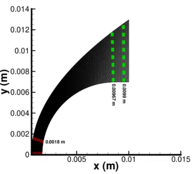
the area considered for optical assessment. . . 56 4.2 Grid Study: Mass density along the stagnation streamline for course,

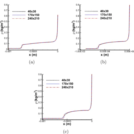
medium, and fine grids shown for (a.) Mach 11, (b.) Mach 13, and (c.) Mach 15. . . 57 4.3 Grid study: mass density in the expansion zone (x=9.7 mm from the

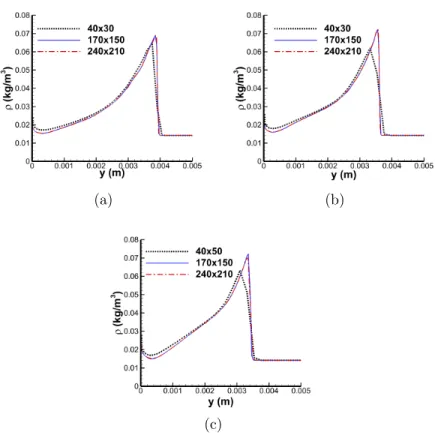
stagnation point) normal to the body for coarse, medium, and fine grids shown for (a.) Mach 11, (b.) Mach 13, and (c.) Mach 15. . . . 58 4.4 Comparison of Mach number contours, (a.) Mach 11 and 13, (b.)

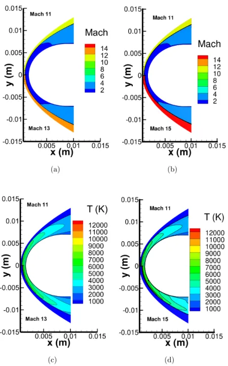
Mach 11 and 15, and comparison of temperature contours, (c.) Mach 11 and 13, (d.) Mach 11 and 15. . . 59 4.5 Comparison of mass fraction contours, (a.) O2 for Mach 11 and 13,

(b.) O2 for Mach 11 and 15, (c.) N2 for Mach 11 and 13, and (d.) N2 for Mach 11 and 15. . . 60

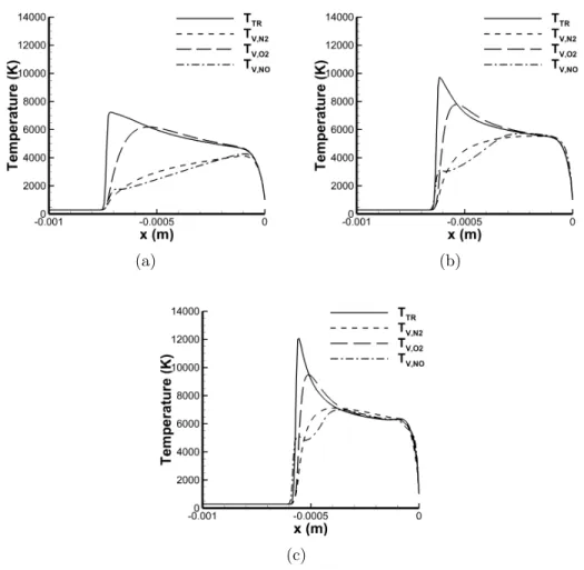
4.6 Temperature Distribution along the stagnation streamline for (a.) Mach 11, (b.) Mach 13, and (c.) Mach 15. . . 61 4.7 Mass Fraction Distribution along the stagnation streamline for (a.)

Mach 11, (b.) Mach 13, and (c.) Mach 15. . . 62 4.8 Temperature distribution normal to the surface at the aftbody (x=9.7

mm from the stagnation point). . . 63 4.9 Mass fraction distribution normal to the surface at the aftbody (x=9.7

mm from the stagnation point). . . 64 4.10 Temperature Contours comparing Real and Perfect Gas Flows at

Mach 11 and 15 . . . 65 4.11 Density profiles in the stagnation region for the Mach 11, (A.), and

Mach 15, (B.), hemisphere flow . . . 66 4.12 Density profiles in the expansion region for the Mach 11, (A.), and

(12)

4.13 OPD profiles for the hemisphere flow: (A.) Mach 11; (B.)Mach 15 in

the stagnation region . . . 68

4.14 OPD profiles for the hemisphere flow: (a.) Mach 11; (b.) Mach 15 in the expansion region . . . 69

4.15 Profiles of the Gladstone-Dale constant along the stagnation streamline. 70 4.16 Comparison of species mass fractions with mass weighted fraction of Gladstone-Dale constant for each species along the stagnation streamline for Mach 15 flow. . . 71

4.17 Profiles of the product of mass fraction and Gladstone-Dale constant along the stagnation streamline at (a.) Mach 11, (b.) Mach 13, and (c.) Mach 15. . . 72

4.18 OPL in the red zone (Fig. 3.1) for (a.) Mach 11, (b.) Mach 13, and (c.) Mach 15. . . 73

4.19 OPD in the red zone (Fig. 1) for (a.) Mach 11, (b.) Mach 13, and (c.) Mach 15. . . 74

4.20 OPL (a.) and OPD (b.) profiles for the Mach 15 flow in the aftbody region. . . 76

4.21 Effects of diffusion along the stagnation streamline for Mach 15 flow on (a.) mass fraction (Zone A), (b.) Gladstone-Dale constant profiles, and (c.) modified index of refraction. . . 77

4.22 OPL (a.) and OPD (b.) with and without diffusion. . . 78

5.1 Counter-rotating vortices used to induce turbulence [10] . . . 82

5.2 Mesh Structure for the Mach 6 Flat Plate . . . 85

5.3 Flat plate density contours (ILES t= 0.25 ms) . . . 86

5.4 Density curves at (a.) x= 0.23 meters and (b.) x= 0.33 meters . . . 87

5.5 Flat plate density profiles for (a.) laminar simulation, (b.) RANS, and (c.) ILES (t=0.25 ms) for Optical Zone . . . 89

5.6 The standard deviation in density for ILES, Menter SST, and laminar flows . . . 90

(13)

5.7 OPD profiles for the flat plate flow . . . 91

5.8 Profiles of OPD obtained from the ILES flow simulation: (a.) in 3 different streamwise planes (t=0.25 ms); (b.) at 3 different time steps (z=0.0129 m) . . . 91

5.9 Velocity profiles for perfect and real gas compared to theoretical curves 95 5.10 Progressive average of TKE for (a.) Perfect Gas and (b.) Real Gas . 96 5.11 Temperature contours for (A.) perfect gas flow and (B.) real gas flow 97 5.12 Density contours for (A.) Perfect Gas and (B.) Real Gas . . . 98

5.13 Density profile at x=0.35 m . . . 99

5.14 Skin friction coefficient . . . 100

5.15 Mass fraction profiles (z=0.0077 meters, x=0.35 meters) . . . 101

5.16 Density fluctuations of perfect and real gas (z=0.0077 m, x=0.35 m) 102 5.17 Index of refraction profile . . . 102

5.18 Optical path distortion . . . 103

6.1 Vortical breakdown characteristic of the Taylor Green Vortex [64] . 108 6.2 Comparison of vortical energy decay for various mesh sizes produced by Hypercode and decay produced WRLES [15] . . . 112

6.3 Vortical break down (as illustrated with vorticity iso-contours) expe-rienced in theO2 perfect gas flow at t=0.01 sec, (a.), t=0.04 sec, (b.), and t=0.10 sec,(c.). . . 114

6.4 Evolution of translational and vibrational temperature for (a.) O2 and (b.) N2 at 4000 K . . . 115

6.5 Evolution of mass fraction for theO2 flow, (a.), and theN2flow, (b.), at 4000 K . . . 116

6.6 Energy evolution for N2, (a.), and O2, (b.), at 4000 K . . . 117

6.7 Turbulent kinetic energy evolution of the Taylor Green vortices of perfect and real gases for N2, (a.), and O2, (b.) . . . 118

(14)

6.8 Evolution in change in kinetic energy for (a.) N2 and (b.) O2 at 4000

K . . . 120 6.9 Vorticity iso-contours forN2 real, (a.), and perfect, (b.), gas

simula-tions at 4000 K . . . 121 6.10 Vorticity iso-contours for O2 real, (a.), and perfect, (b.), gas

simula-tions at 4000 K . . . 122 6.11 Density iso-contours for N2 real, (a.), and perfect, (b.), gas

simula-tions at 4000 K . . . 123 6.12 Density iso-contours for O2 real, (a.), and perfect, (b.), gas

(15)

LIST OF TABLES

Table

2.1 S-A Constants . . . 21

2.2 Species’ Gladstone-Dale Constants . . . 27

3.1 Common Radio Frequencies used for Communication . . . 41

3.2 Study Flow Parameters . . . 42

3.3 Strehl ratios produced by method I . . . 48

3.4 Strehl ratios produced by Method II . . . 49

4.1 Test Conditions . . . 55

5.1 Turbulence Study Flow Parameters . . . 84

5.2 Flat plate Mesh Parameters . . . 84

5.3 Mach 4 Test Case Flow Parameters . . . 93

(16)

LIST OF ABBREVIATIONS

Dsk Multicomponent Diffusion Coefficient

e Energy [J/kg]

h Enthalpy [J/kg]

k Thermal Conductivity [W/(m· k)]

kb Backward Rate Coefficient

KEQ Equilibrium Rate Coefficient

kf Forward Rate Coefficient

KGD Gladstone-Dale Constant [m3/kg]

l Coordinate along Line of Sight [m]

Le Lewis Number

M Mach Number

n Index of Refraction

OPD Optical Path Difference [m]

OPL Optical Path Length [m]

P Pressure [Pa] ˙ q Flux Vector [W/m2_] ρ Density [kg/m3] T Temperature [K] t Time [s] θ Characteristic Temperature [K] τ Relaxation Time [s] ˜

τ Shear Stress [Pa]

u Diffusion Velocity [m/s] u Velocity [m/s] ˙ ω Source Terms X Molar Fraction Y Mass Fraction

tke Turbulent Kinetic Energy

Sc Schmidt Number

Rs Strehl Ratio

λ Wavelength [m]

f Frequency [Hz]

(17)

Sub/Superscripts c Controlling d Dissociation ∗ Equilibrium ∞ Freestream hi Spatial Average s Species 0 _Fluctuating trans Translational t Turbuelent v Vibrational radio radio chem Chemical r Rotational

(18)

ABSTRACT

A potential future use of hypersonic platforms is for responsive Intelligence, Surveil-lance, and Reconnaissance (ISR). It is common for these types of missions to employ Electro-Optical/Infrared (EO/IR) sensors and Radio Frequency (RF) sensors to col-lect information. If an optical signal were to travel through a hypersonic flowfield, the type of high-speed flow analysis required to perform reliable assessments of sen-sor performance is unclear. In order to provide this information, the hypersonic flow phenomena of thermochemistry, high speed turbulence, and high enthalpy turbulence are studied.

In a hypersonic environment, the high kinetic energy of the oncoming flow causes the molecules in the flow to be thermally excited, leading to dissociation. In such a flowfield, an aero-optical analysis that considers thermochemical nonequilibrium is necessary to assist in sensor design. In the present thesis, we assess the optical properties of a nonequilibrium flowfield. The optical distortions are quantified using optical path length (OPL) and optical path difference (OPD). Optical distortion is also assessed based on flowfield modeling performed using a perfect gas assumption, and these distortions are provided for comparison. The primary contributions of nonequilibrium flow properties on optical distortion are identified. For all Mach numbers, OPLs are higher when the effects of dissociation and vibrational relaxation are included. Oxygen dissociation is the dominant nonequilibrium flow phenomenon affecting the optical distortion. As Mach number increases, atomic nitrogen begins

(19)

to have an additional influence on optical aberrations.

Additional distortion can arise in the hypersonic regime from high speed turbu-lence within the boundary layer. An initial study is conducted on a Mach 6 flow over a flat plate. This simulation is performed using air as a calorically perfect gas with varying levels of turbulence modeling and resolution. The cases are run using a laminar flow assumption (no turbulence), the Menter SST closure model for the Reynolds Averaged Navier-Stokes equations (RANS), and Implicit Large Eddy Sim-ulation (ILES). It was found that the OPDs produced by the highest fidelity ILES approach can be as much as two orders of magnitude larger than solutions produced by the Menter SST model and laminar flow. While RANS was able to predict the mean flow quantities, it is unable to correctly predict the optical distortion.

The effects of thermochemical nonequilibrium on turbulent flow, and consequently optical distortion, are also presented in this dissertation. In the present study, numer-ical simulations are utilized to perform implicit large eddy simulations of flows over an adiabatic flat plate. The simulations are run with and without thermochemistry models to determine the effects of thermochemical nonequilibrium on optical distor-tion. Accounting for thermochemical nonequilibrium predicts less variation in OPD across the sensor aperture. The RMS average of OPD is significantly smaller for the real gas simulation when compared to a perfect gas. These differences in OPD occur because nonequilibrium energy exchanges act to damp out turbulent fluctuations, as illustrated with the Taylor-Green Vortex problem in this thesis. It is therefore neces-sary to include these physical flow effects in optical assessments to obtain an accurate description of the aero-optic distortions.

(20)

CHAPTER I

Introduction

1.1 Motivation

Throughout history, man has desired to fly further in less time. As such, much time and effort has been devoted to the pursuit of technological advances in the field of aeronautics. As technology advances, flight in the hypersonic regime is becoming more feasible. Missions for vehicles engaged in intelligence, surveillance, and reconnaissance (ISR) are well suited for hypersonic flight. Hypersonic ISR vehicles will be able to collect accurate and time relevant information to support missions globally. Figure 1.1 presents an image of a proposed hypersonic vehicle that is designed for ISR missions by the Boeing Corporation [11]. Sensors placed on vehicles like those in Fig. 1.1 are particularly susceptible to distortion, as the flow around such a body often reduces

(21)

the effective range of the sensor [58].

Numerous aspects of any flowfield can be a potential cause of signal distortion and aberration. This is especially true when examining hypersonic flow phenomena. One such type of distortion is radio frequency (RF) sensor degradation, often referred to as radio blackout. This phenomenon occurs when enough energy is imparted onto the air molecules that they not only dissociate, they begin to ionize. Radio waves can be reflected or diminished by the plasma layer [31]. Any signal with frequencies that fall below the characteristic plasma frequency will be attenuated [31]; as such, low frequency RF signals are the most vulnerable.

Radio blackout is a problem that has and continues to plague vehicles engaged in space travel. The Apollo missions experienced lost communications, for example [31]. Figure 1.2 presents a depiction of the Apollo re-entry trajectory. The altitudes at which the capsule experienced loss of communications are denoted in the figure. The altitude traversal where radio blackout was experienced corresponds to a time

Figure 1.2: Apollo re-entry trajectory [31]

period of several minutes. Even modern re-entry vehicles can expect anywhere from 4 to 16 minutes of radio blackout [31]. While the ISR platforms are intended to fly intra-atmospheric missions, blackout may still be an issue since these vehicles will experience strong shock waves with elevated temperatures.

(22)

Another type of signal distortion that requires in-depth analysis is the distortion of an electo-optical or infrared (EO/IR) signal collected or sent from a hypersonic vehicle. Optical distortion caused by a flowfield is seen frequently in phenomena such as the twinkling of stars and is leveraged in the collections of Schlieren and shadowgraph images [57]. Distortion of an EO/IR beam arises as the beam travels through a field consisting of varying indices of refraction (which can be found from the density and mass fraction profiles using the Gladstone-Dale relation) [20]. Portions of an initially coherent wave front travel at different local speeds throughout such a field. A sensor used to detect through this field, therefore, will receive a signal that has various portions which have experienced phase shifts. An initially coherent structure will no longer be so. These aberration effects can be even larger in the presence of turbulent flow, as this type of flow is highly chaotic. Figure 1.3 presents a schematic of the optical distortion experienced from a sensor placed on a turret-like structure which is immersed in a turbulent flow.

Figure 1.3: Schematic of Aero-optical distortion [57]

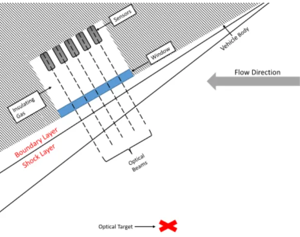
It should be noted that the EO/IR signal sent or received by a sensor located on the surface of a body will experience many effects apart from those imposed directly by the vehicle’s interaction with the fluid around it. Figure 1.4 presents a description of various sources of possible signal distortion. Possible sources of distortion arise from the gas within the sensor, the sensor window which is often exposed to high

(23)

Optical Target

Flow Direction

Figure 1.4: Schematic of possible sources of EO/IR signal distortion

temperatures, the boundary layer, the shock layer, and the atmosphere. The majority of the study presented in this dissertation focuses on the aero-optical effects, or the effects imposed on the signal from the boundary layer and the shock layer. The effects from the window and the atmosphere are neglected.

1.2 Review of Relevant Work

Many approaches have been taken to quantify sensor distortion, some of which are mentioned in Chapter III through Chapter VI. The study of aero-optics within the United States has gone through two stages of evolution, each of which coincided with developments in the field of laser technology [29]. The first period began in the 1970’s and lasted until the 1980’s. The second period began in the early 1990’s and represents the era we are currently in [29]. The first era of study was primarily concerned with turrets and beam detectors as well as with atmospheric effects. As such, much study was dedicated to predicting the optical distortion produced in free shear flows. Many of the methods used to quantify optical distortion that are still used today were developed during this period. The Strehl ratio, or the ratio of the intensity of a distorted beam to an undistorted one, first made its appearance during the first period of aero-optical discovery [29].

(24)

The second period in which we are now in is marked by the advancement technol-ogy. For example, wave sensor technology has improved to a point at which taking detailed measurements in experimental settings is possible. Another important ad-vancement in the second era can be found in the computational sciences. Solving higher fidelity flow models is now possible. The existing work still often details the optical distortion caused by turrets in sub- or supersonic flow [29]. Due to the flow scales in these test cases, the flow is treated as turbulent. Another set of current computational work focuses on relatively low speed, low enthalpy turbulent bound-ary layers created over flat or near-flat surfaces [57], [22], [23]. Only recently, as technology has advanced, has optical distortion analysis included resolved turbulence analysis. It is common in these studies to present the total distortion in terms of optical path difference, an approach which is adopted in the current study [57].

Much of the prevailing hypersonic work in the field of aero-optics is computa-tional in nature, as it is expensive and very hard to replicate flight enthalpies. Often, the media surrounding a hypersonic vehicle is at a high temperature and cannot be accurately represented by a perfect gas. In fact in Ref. 1, it is illustrated that for any temperature exceeding 5000 K a single Gladstone-Dale constant, a proportion-ality constant used to find index of refraction, cannot describe the entire flow field. Atomic species will increase the Gladstone-Dale constant more than their molecular counterparts, as they have higher individual Gladstone-Dale constants [1]. While Ref. [30], does use density averaged Gladstone-Dale constants, the assessment is restricted to shock tunnel simulations. Algebraic relations to obtain OPDrms have been developed for this regime of flow, however, they are limited in application [63], [23]. For example, Ref. 58 is derived for an adiabatic wall assuming turbulence and small pressure fluctuations. Similar to these, many studies are concerned largely with turbulent fluctuations in the supersonic regime [22], [57]. The published data also does not provide any information regarding the sensitivity of optical quantities to

(25)

nonequilibrium flow phenomena. From the published data, the effects of including nonequilibrium in optical calculations is not immediately apparent.

Studies that investigate the interaction between turbulence and chemical reac-tions are scarce. The few studies that do exist have shown that turbulence may exert a significant effect on detailed chemical composition [36]. Furthermore, these stud-ies show that exothermic reactions increase turbulent fluctuations and endothermic reactions dampen turbulent fluctuations. In the boundary layer, both types of re-actions are possible, as species may dissociate and recombine. It should be noted that these past studies neglected thermal nonequilibrium. Even fewer studies have investigated a turbulent flow in thermochemical nonequilibrium to calculate optical properties. Most studies focus on low enthalpy perfect gas flows. The flow media surrounding a hypersonic vehicle cannot be accurately represented by a perfect gas. None of these simulations investigate the manner in which thermochemical nonequi-librium effects optical distortion in turbulent flows. Wyckham and Smits did present optical distortion over a flat plate for a turbulent flow with a high Mach number [63]. However, detailed descriptions of the role of thermochemical nonequilibrium in optical distortion is lacking in the published data and is a focus of the present thesis.

1.3 Background

Section 1.2 is presented in two subsections, each providing background information regarding flow phenomena that may have a significant effect on signal distortion.

1.3.1 Hypersonic Flight Conditions

The very definition of hypersonic flow is under much contention. Unlike sub- and supersonic flows, which are clearly delineated on the basis of Mach number, there are no clear Mach number divisions at which all flow above is hypersonic. As Pro-fessor P.L. Roe stated with regards to the definition of hypersonics, “it would be

(26)

quite possible for someone to advocate, and defend, numbers as small as three, or as high as 12. [2]” Instead, the definition of the hypersonic regime relies on the appear-ance of certain physical flow phenomena. These phenomena become progressively important as Mach number increases [3]. The flow phenomena that are of special importance in hypersonic flows are thin shock layers caused from increased density post-shock and the conservation of mass, strong entropy gradients within the bound-ary layer caused from the strong shock surrounding the vehicle body, and the strong viscous interactions (within the shock) that result in thick boundary layers with very high translational temperatures. These elevated temperatures can excite the internal modes of the molecules. Above 800 K, the vibrational mode of molecules becomes ex-cited; beginning at 2000 K molecules in air begin to dissociate; starting at 9000 K the atoms in air can begin to ionize (Chemical dissociation and ionization are presented at equilibrium conditions) [4]. The excitation of the internal modes has ramifications on the bulk flow properties and, consequently, the optical distortion produced by the field.

Figure 1.5 presents the shock layer temperature for various re-entry velocities [2]. In the figure, the calorically perfect predicted shock temperature is also provided. The chemically reacting boundary layer has lower post-shock translational temperatures. This lowering of temperature is a consequence of energy leaving the translational mode and entering the excited internal modes. While Fig. 1.5 presents the effects of an equilibrium chemically reacting boundary layer, reaching equilibrium requires some amount of time. When the flow passes through high gradient regions, it takes a finite amount of collisions for the internal energies to adjust to a new thermodynamic state, often resulting in regions of nonequilibrium and relaxation [55]. Vibrational and chemical energy exchange processes are often relatively slow (compared to trans-lational and rotational energy exchange processes), as seen in Eqn. (1.1) , to adjust

(27)

Figure 1.5: Comparison of temperature ratios between a calorically perfect gas and reacting flows [2]

to the rapidly changing flowfield, and thus nonequilibrium in these modes prevail.

τchem, τv >> τtrans, τr (1.1)

where τ is the characteristic time scales of the various flow phenomena.

In nonequilibrium regions, chemical dissociation often begins when the freestream Mach number of the vehicle exceeds 6. Dissociation occurs when the internal energy exceeds the dissociation energy of the molecule. Therefore, dissociation depends on the state of the internal energy modes and consequently the relaxation processes [26]. Through the gas transport processes, species can also diffuse, further altering the gas flow properties.

To accurately assess signal propagation through a hypersonic flowfield, high en-thalpy flow physics need to be appropriately accounted for in optical distortion pre-diction. Specifically, high enthalpy effects in high gradient regions, such as strong shocks and boundary layers, need to be addressed in the optical assessments.

(28)

1.3.2 Turbulence

Because we are interested in examining the effect of hypersonic flow on optical distortion, it is pertinent to study turbulence in addition to high enthalpy thermody-namics. In particular, it is important to understand the manner in which energy is distributed and stored in turbulent flows, and how this can be affected by hypersonic flow phenomena. The turbulent energy can have an effect on optical analysis because turbulence is a chaotic flow phenomenon; it consists of vortical structures which pro-mote fluctuations in flow parameters both spatially and temporally. These flows are often non-homogenous and anisotropic.

As an example of the complexity associated with turbulent flows, the precise definition of the turbulent structures, commonly referred to as eddies, has remained elusive to scientists [46]. Instead, eddies have come to be largely recognized as regions of turbulent motion which are relatively organized and have a consistent structure [46]. The eddies can range in size from the large scale eddies which have sizes dictated by the characteristic length associated with the general flow under consideration down to the smallest scales which can be dissipated by viscous effects. The larger eddies can occupy regions that are also populated by eddies of smaller sizes.

In 1920 Richardson proposed that the large eddies are inherently unstable [24]. As a consequence of this, the eddies break down into multiple smaller eddies (consis-tent with the stretching and conservation of angular momentum present in turbulent flows). This process will continue until the eddies become small enough for the vis-cous forces to have any influence over them. When the eddies reach the smallest “stable” scales, the viscous forces begin to dissipate the organized turbulent motions. Richardson hypothesized that the largest eddies are responsible for the energy pro-duction in turbulence, these eddies then break down and transfer energy through invisicid processes, due to the instability of their structures, to the smallest eddies which are dissipated by the viscosity.

(29)

Kolmogorov expanded upon (and quantified) these ideas; he developed what has come to be known as K-41 theory [46]. This theory is based on physical logic and has proven to be helpful in describing the general structure of turbulent flows [46]. Kolmogorov presented the idea that all geometric information of the large eddies is lost as the eddies break down in size, and, consequently, the smaller scales are statistically independent of the larger eddies. Therefore, the smaller scales are independent of the mean flow and the boundary conditions. He argued that the motions of these small scale eddies are universal to all turbulent flows. He further presented the idea that turbulent structures are dependent on only viscosity and dissipation rate (ν and ε, respectively) since they represent the two dominant processes that dictate energy transfer in turbulent flows. Kolmogorov further built upon this idea by supposing the intermediate scales have sufficiently high Reynolds numbers that the viscous effects are negligible on their energy transfer. This means that at sufficiently high Reynolds numbers, the intermediate scale are dependent on only ε. This correlates well with the hypothesis posed by Richardson, that energy is injected into turbulence at the large scales and cascades through intermediate structures until the structure is small enough for the viscous force to have a significant influence on them. Using dimensional analysis, energy in this range can be represented only by Eqn. (1.2).

E(k) =Ckε

2 3k

−5

3 (1.2)

where Ck is referred to as the Kolomogorov constant and k is the wavenumber. The

implications of K-41 theory are of importance. K-41 theory suggests that in all turbulent flows there is a universal range where energy decays at a rate of k−35.

Figure 1.6 presents the scaled energy spectrum for turbulent flows.

The purpose of discussing the turbulent energy cascade are two-fold. One reason to understand this cascade is to gain insight into turbulence modeling; see Chapter II

(30)

Figure 1.6: Turbulent energy spectrum [50]

for information regarding the specific models used in this study. Methods for perform-ing turbulent calculations range from Reynolds-Averaged Navier-Stokes (RANS), in which all turbulent dynamics are modeled, to direct numerical simulations (DNS), in which all scales shown in Fig. 1.6 are resolved. Large eddy simulation (LES) lies in between these two methods in terms of resolution. Large eddy simulation resolves all large energy-containing eddies and all eddies in the universal inertial range; see Fig. 1.6. All small, dissipative scales are either modeled or numerically dissipated.

The other reason to study the turbulent cascade is to better understand energy ex-changing mechanisms in turbulent flow and how they may be affected by thermochem-ical nonequilibrium. While studies that investigate turbulence and thermochemthermochem-ical nonequilibrium are not numerous, it is largely supposed that any mechanism which extracts energy out of the translational mode will dampen turbulent structures and turbulence in the inertial range may no longer be universal. Studying the turbulent energy transfer produced from simulations which utilize thermochemical nonequil-brium models can, therefore, provide insight into how these features affect turbulent flow and consequently optical distortion.

1.4 Scope of Present Work

The present work is divided into seven chapters. Chapter II presents the numerical analysis, both of the flowfield and of the optical distortion, employed in this study.

(31)

Chapter III presents a preliminary assessment of possible causes of signal distortion. Chapter IV illustrates the effects of modeling thermochemical nonequilbrium on signal distortion. Chapter V illustrates the effects of high velocity turbulence on signal aberration. Due to the importance of turbulence on optical distortion, it is pertinent to discuss the manner in which turbulent flow can be affected by thermochemical nonequilbrium. Chapter VI presents the effects of thermochemical nonequilibrium on turbulent flow. Chapter VII presents a summary discussing the ways in which hypersonic flow phenomena affect signal distortion.

(32)

CHAPTER II

Numerical Methods

2.1 Introduction

This chapter details the methods utilized in this study to simulate both the mean flow and optical solutions. This numerical analysis is presented in two sections, (1) nonequilibrium computational analysis of the flow field around the body of interest (including the nonequilibrium models used in this study), and (2) optical assessments using both real and perfect gas Gladstone-Dale proportionality constants.

2.2 Flowfield

The flowfield calculations are discussed in terms of (a) The Navier-Stokes equa-tions with nonequilbrium models and (b) the modeling and resolution of turbulent structures.

2.2.1 Nonequilibrium Flow Field Calculation

The numerical calculations are conducted using computational fluid dynamic codes developed for high speed applications in which the Navier-Stokes equations are coupled with thermodynamic and transport property models. Unless otherwise noted, the information presented in this work pertains to all codes that are used.

(33)

The majority of this study is conducted using the research codes LeMANS (see Ref. [59] for validation and verification), US3D (see Refs. [40], [41] for validation and verification studies), and ANDEE (see Refs. [28], [27] for validation and verification studies). The computations are performed with the aid of finite rate chemistry and the Landau-Teller vibrational energy relaxation model. The mass-averaged velocity form of the governing equations for nonequilibrium flow are given in Eqns.(2.1) - (2.4) [27]. Unless otherwise noted, variables are as described in the list of abbreviations.

∂ ∂tρs+∇ ·ρs(u+us) = ˙ωs (2.1) ∂ ∂tρu+∇ ·(ρuu+ ˜τ) = 0 (2.2) ∂ ∂tρsev,s+∇ ·(ρsev,s+ρs(u+us) + ˙qv,s) = ˙ωv,sρs+ev,sω˙s (2.3) ∂ ∂tρe+∇ ·(ρ(e+ P ρu))−q˙trans− X ˙ qv,s+ X (ρshsus) =∇ ·(uτ˜) (2.4)

Eqn. (2.1) is the species’ mass conservation equation. In Eqn. (2.1), ρs is each species’ density, and us is the diffusion velocity. The diffusion velocity is assumed to

be generated by the species’ concentration gradients according to Fick‘s first law of diffusion [6]:

ρsus=−ρDsk∇

ρs

(34)

where Dsk is the multicomponent diffusion coefficient and assumes a constant Lewis

number of 1.4.

Le= ρDskCp

k (2.6)

In Eqn.(2.1), the creation and destruction of each species, s, is represented by the source term ˙ωs. This source term used to describe chemical nonequilibrium

(neglect-ing ionization) is found for each species utiliz(neglect-ing the 17 reactions (see Eqns.(2.7)) that occur with the 5 primary species in dissociating air (N2, O2, N O, N, and O).

In Eqns.(2.7), M represents all 5 collisional partners.

N2+M ↔2N +M (2.7a)

O2+M ↔2O+M (2.7b)

N O+M ↔N+O+M (2.7c)

N O+O ↔O2+N (2.7d)

N2+O ↔N O+N (2.7e)

The first three reactions (a−c) in Eqns.(2.7) represent the dissociation and recom-bination of N2, O2, and N O, respectively. The last two reactions in Eqns.(2.7) are

exchange reactions involving N O. In equilibrium, oxygen begins to dissociate at about 2000 K, followed by nitrogen at 4000 K. N O forms at approximately 2000 K through dissociatedO colliding with the abundant N2 molecules (via Eqn.(2.7e)) [2]. N O will begin to dissociate at higher energies than O2 due to the strength of the

bond that is formed between the nitrogen and oxygen atom[9]. The forward reaction rate and backward reaction rates are given in Eqns.(2.8) and (2.9), respectively. The

(35)

equilibrium constants and reaction rate coefficients are taken from Park [45]. kf(Tc) =CfTcηexp( θd Tc ) (2.8) kb(Tc) = kf Keq (2.9)

where Keq is derived from statistical mechanics and is referred to as the equilibrium rate coefficient and Tc is the rate controlling temperature; see Eqn.(2.10) [43].

Tc=

p

(T Tv) (2.10)

whereT is the translational temperature andTv is the vibrational temperature. This

model is referred to as Park‘s two temperature model [43]. It should be noted that in this study it is assumed that the flow is in rotational equilibrium. Equation (2.2) is the total momentum conservation equation. Equation (2.3) is the vibrational en-ergy conservation equation which incorporates terms to describe vibrational enen-ergy conduction and diffusion. The source term for the conservation of vibrational en-ergy equation is found using the Landau-Teller Relaxation model which describes vibrational translational energy coupling; see below [32].

˙

ωv,s =ρs

e∗_v,s−ev,s τs

(2.11)

where ˙ωv,sis the energy exchange rate for the vibrational mode,e∗_v,sis the equilibrium vibrational energy of species s at the local translational temperature, and ev,s is the

(36)

Eqn.(2.12). τs = P sXs P sXs/τrs (2.12)

where Xs is the mole fraction of the species s. The inter-species relaxation time,τrs , is found using the Millikan and White approximation; see Eqn.(2.13) [38].

pτrs= (−18.42) + (1.16x10−3)µ 1 2θ 4 3 v,s(T− 1 3 −0.015µ 1 4) atm·s (2.13)

LeMANS, which is used for Chapter III, utilizes an additional correction factor in the Millikan and White approximation suggested by Park [43]. The vibrational temper-ature for each species is determined with a known vibrational energy and Eqn.(2.14) [55].

ev,s = Rθv,s

exp(θv,s/Tv,s)−1

(2.14)

where R is the species gas constant and θv,s is the characteristic temperature of

vi-bration for each species, s. Equation (2.4) is the total energy conservation equation which includes additional terms that describe the species diffusion and translational heat conduction. Equations (2.1) - (2.4) are solved using the finite volume formu-lation. The viscosity for each species is found using Blottner curve fits [7], and the thermal conductivity for each species is found using Euckens relations [55]. Wilkie‘s semi-empirical mixing rule is used for the conductivity and the viscosity of a mixture [60].

It should be noted that Park‘s two temperature model was developed based on experimental investigations and may not accurately describe flow with rotational nonequilibrium and significant radiation that induces ionization [44]. The Landau-Teller model assumes only weak deviations from equilibrium. It also assumes the

(37)

molecules behave as a simple harmonic oscillator, and it only allows for single quantum jumps [55]. Millikan and White relaxation times were derived from empirical curve fits that do not accurately represent high temperature nonequilibrium physics [9]. The data for these curve fits are collected from shock tube experiments performed at temperatures ranging from 300 K to 8000 K [38]. Because of the narrow temperature range used to derive the fit, the curve fit only reports relaxation at certain vibrational levels. Still, these models are adequate for assessing a number of nonequilibrium phenomena and are widely used to describe nonequilibrium physics, thereby allowing a preliminary assessment of the effects of nonequilibrium on optical calculations.

2.2.2 Turbulence

Two classes of turbulent simulations are employed in this thesis. The Reynolds Averaged Navier Stokes equations are solved, and large eddy simulations are per-formed.

2.2.2.1 Reynolds Averaged Navier Stokes Equations

One of the most prevalently used methods utilized to assess turbulent flows in-volves decomposing the velocity into a mean and a fluctuating component. This sum of the two components is then inserted into the Navier-Stokes equations and the aver-ages of the equations are taken. The resulting set of equations is called the Reynolds Averaged Navier Stokes equations (RANS); see appendix A for full description of these equations [21].

In the RANS equations there are more unknowns than there are equations, as such these equations cannot be directly solved. The inability of RANS to be solved by themselves is commonly referred to as the closure problem and arises from the existence of an additional stress referred to as the Reynolds stress. One method that is used to “close” these equations finds its basis in the Boussinesq equation; see

(38)

Eqn.(2.15) [24]. −ρ(u0_iu0_j) = µt( ∂ui ∂xj +∂uj ∂xi − 2 3 ∂uk ∂xk δij)− 2 3ρkδij (2.15)

This model assumes that the Reynolds stress can be modeled in an analogous manner to the laminar stress. It should be noted that in Eqn.(2.15),δijis the kronecker delta

function and k is the turbulent kinetic energy.

With the aid of Eqn.(2.15) the RANS equations largely take the form of the laminar Navier-Stokes equations with the conserved variables describing the mean flow field. Notable differences in the equation sets (RANS and Navier-Stokes) can be found in the modification of the stress term in the conservation of momentum equation [21].

∂ ∂xj

(tij +τij) (2.16)

where τij is the turbulent stress and is of the form suggested by Boussinesq; see

Eqn.(2.15).

The energy equation is modified by the addition of the term shown in Eqn.(2.17) which represents the effect of turbulent shear stress on the system’s energy.

∂ ∂xj

(ui(tij +τij)) (2.17)

It should be further noted that the diffusion coefficient and thermal conductivity are also modified to include the effects of turbulence in the flow. The total diffusion coefficient and thermal conductivity are now composed of the sum of their respec-tive laminar and turbulent components. The turbulent translational and vibrational

(39)

thermal conductivities are presented in Eqns.(2.18) and (2.19) [21]. kturb = klam klam+kv,lam µt cpP rt (2.18) kv,turb = kv k+kv µt cpP rt (2.19)

where P rt is the turbulent Prandtl number and is taken to be 0.9, as suggested by

Allmaras [52]. The turbulent contribution to diffusion is shown in Eqn.(2.20).

Dt= µt

ρSct (2.20)

where Sct is the turbulent Schmidt number and is assumed to be constant andµt is

the eddy viscosity. The eddy viscosity is as of yet unknown. A further model must be used to find this effective turbulent viscosity. One such model, based largely on empiricism and dimensional arguments, is the Spalart-Allmaras model (S-A model) [52].

The S-A model consists of one equation that describes the transport of a modified turbulent (eddy) viscosity. At its inception, it was assumed that an incompressible eddy viscosity model would be sufficient in the compressible regime. This was proved to be incorrect. The S-A model was thus improved as shown in Eqn.(2.21) [13].

∂ρν_e ∂t +uj ∂ρ_eν ∂xj =cb1(1−ft2)Sρe eν− h cw1fw− cb1 κ2ft2 i ρ e ν d 2 + 1 σ ∂ ∂xj ((µ+ρν_e)∂νe ∂xj ) +cb2ρ ∂ν_e ∂xi ∂ν_e ∂xi (2.21)

In Eqn.(2.21),Seis the modified vorticity; see Eqn.(2.22).

e

S ≡S+ eν

(40)

where dis the distance to the closest wall, S is the magnitude of vorticity, andfv2 is

found using Eqn.(2.23).

fv2 = 1− χ

1 +χfv1

(2.23)

In the S-A model, fw is found using Eqn.(2.24).

fw =g 1 +c6 w3 g6 ₊_c6 w3 1₆ (2.24)

where g is found using Eqn.(2.25) and Eqn.(2.26).

g =r+cw2(r6−r) (2.25)

r=min( ν˜

e

Sκ2_d2,10) (2.26)

The term ft2 is described in Eqn.(2.27).

ft2 =ct3exp(−ct4χ2) (2.27)

All remaining constants are described in Table 2.1 [52].

Table 2.1: S-A Constants Constants Value cb1 0.1355 σ 2/3 cb2 0.622 κ 0.41 cw1 cb1/κ2+ (1 +cb2)/σ cw2 0.3 cw3 2 cv1 7.1 ct3 1.2 ct4 0.5

(41)

The S-A model, as shown in Eqn.(2.21), can allow negative eddy viscosity which presents a non-physical solution. This anomaly is caused from grids that do not properly resolve the flow and non-physical variations in time that can arise from dis-cretization schemes. In order to avoid negative eddy viscosity, the modified vorticity as described in Eqn.(2.22), is altered. The improved vorticity model is shown in Eqn.(2.28). e S=        S+ ¯S S¯≥ −cv2S S+ S(c2v2S+cv3S¯) (cv3−2cv2)S−S¯ ¯ S <−cv2S (2.28) where ¯ S= eν κ2_d2fv2 (2.29)

and S is the magnitude of vorticity. The variables found in Eqns.(2.29) and (2.28) are as described above with the addition of cv2 which equals 0.7 andcv3 which equals

0.9.

Another modification is implemented to avoid further undershooting. This modi-fication consists of utilizing a different conservation equation if the eddy viscosity is less than zero. The negative model takes the form of Eqn.(2.30) [52].

∂ρν_e ∂t +uj ∂ρ_eν ∂xj =cb1(1−ct3)Sρe e ν−cw1ρ e ν d 2 + 1 σ ∂ ∂xj ((µ+fnρνe) ∂ν_e ∂xj ) +cb2ρ ∂_eν ∂xi ∂ν_e ∂xi (2.30)

When compared with Eqn.(2.21), Eqn.(2.30) is found to be similar with changes to few terms. The function fn is introduced and found using Eqn.(2.31).

fn =

cn1+χ3 cn1 −χ3

(42)

where cn1=16 and χ is as described above.

Using Eqns.(2.30) and (2.21), the eddy viscosity can be found directly using Eqn.(2.32).

µt =ρνfe v1 (2.32)

where fv1 is found using Eqn.(2.33).

fv1 = χ3 χ3 ₊_c3

v1

(2.33)

and cv1 is equal to 7.1. χ is described in Eqn.(2.34).

χ= νe

ν (2.34)

In order to be numerically evaluated, the S-A convective fluxes (see Eqn.(2.35)) are discretized and shown in Eqns.(2.36). The fluxes are discretized using integration over a surface and an upstream method in which the variables from the direction upstream in the flow are used and those downstream are neglected.

∇ ·(ρ~u_eν) (2.35)

X

0.5∗(ulef t+uright)ρeνupstreamds (2.36)

where ulef t and uright denote the values of u in each respective cell and ds denotes

the area of the face.

(43)

a surface as shown in Eqn.(2.38). 1 σ((µ+ρνe)∇eν) (2.37) 1 σ X (µ+¯ρ_eν)(∇_eν·n)ds (2.38)

The final term in the S-A model that is discretized is the cross diffusion term; see Eqn.(2.39). cb2 σ ρ∇ 2 e ν (2.39)

The cross diffusion term was discretized using the divergence theorem and values of eddy viscosity from the right and left cells of each face. The fullly discretized term is illustrated in Eqn.(2.40). cb2 σ X (ν_elef t+eνright) 2_ρ_∗_V _(2.40)

The dependence on volume in the previously shown term evolves from integrating over a control volume.

The source terms are algebraic in nature and require no extra treatment from their original form (in Eqn.(2.21)) except for integration over a control volume.

Once the terms are discretized in space, an implicit time-marching scheme is constructed for the model. For demonstration of this application the S-A model is presented in a compact form; see Eqn.(2.41).

V ∂ρνe

∂t =−R (2.41)

(44)

commonly referred to as the residual. V, which denotes cell volume, appears through the discretization process when terms are integrated over a control volume. The implicit time marching method is applied as in Eqn.(2.42).

V

4tρ(νen+1−νen) =−R(˜νn+1) (2.42)

The right side of Eqn.(2.42) is then expanded using a Taylor series. Higher order terms are neglected, and Eqn.(2.43) is obtained.

R(_eνn+1) = R(eνn) +

∂R

∂ν_e4eν (2.43)

Equation 2.42 can then further be simplified to Eqn.(2.44).

( V 4tρ+

∂R

∂_eν)4eν =−R(eνn) (2.44)

Equation (2.44) provides a method to find the updated viscosity (from 4_eν) with the described spatial discretization. A previously undiscussed term appears in Eqn.(2.44),

∂R

∂ν˜, which is called the Jacobian.

The Jacobians for the source terms depend on taking the derivative of each func-tion with respect to the conserved variable. In practical applicafunc-tions, the cross diffu-sion contribution to the Jacobian are neglected due to stability issues that can occur. The Jacobians for the convective and diffusive fluxes are differential in nature and found as in Refs. [14].

2.2.2.2 Large Eddy Simulation

While RANS is able to capture mean flow behavior with some reliability, it uses simplistic approximations to assess flow features and is unable to provide resolved turbulent information. Due to the lack of detail provided by RANS simulations, it is

(45)

necessary to utilize the more computationally expensive large eddy simulation (LES). LES utilizes the Navier-Stokes equations applied to a filtered flowfield to solve for a system on a mesh with enough resolution to resolve the large-scale turbulent struc-tures. The small scale turbulence is either modeled or dissipated by the grid spacing. Due to the computational expense related to this method of solution, relatively sim-plistic flows are evaluated.

The flat plate large eddy simulations in this thesis are conducted using the finite volume US3D code, a computational fluid dynamics code for high speed flows that was developed at the University of Minnesota. In US3D, the viscous terms are calculated using a 2nd-order central scheme. The inviscid terms are calculated using a 6th-order central scheme. The time integration is performed using a 2nd-order implicit method. The high order terms are used to help reduce the number of grid points required in the computational domain to resolve the turbulence [53].

The Taylor-Green vortex problem in this study is run with Hypercode. It is a finite volume code intended for use on high speed flow applications. Hypercode uses a 2nd-order central scheme for the viscous fluxes and 5th-order weighted essentially non-oscillatory (WENO) stencil (with AUSM flux splitting) for the inviscid fluxes. Hypercode uses a second order explicit time-marching scheme.

The large eddy simulations are conducted using an implicit filter. An implicit LES method does not resolve all turbulent flow features. Instead, the grid behaves as a filter. All features that are not resolved by the grid will be numerically dissipated [19]. This level of resolution is acceptable for an optical study because the most optically important features are approximately the size of the boundary layer [58].

2.3 Optical Analysis

The optical analysis is performed on a steady-state flow field. To conduct optical assessments of an initially planar wave front, the index of refraction of the fluid

(46)

mixture surrounding the vehicle is needed. The index of refraction can be found from simplifying Lorentz radiation interaction theory with the model of an induced harmonic oscillator [51]. The resulting simplification for transparent media is the Gladstone-Dale relation; see Eqn.(2.45) [61]:

n =KGDρ+ 1 (2.45)

where n is the index of refraction, ρ is the gas mixture density and KGD is the

Gladstone-Dale constant. The Gladstone-Dale relation is built upon Lorentz radiation interaction theory. The Gladstone-Dale constant in Eqn. (2.45) can be assumed to be a constant for the entire flowfield as for (perfect gas) air. However, this study also uses a Gladstone-Dale constant that is variable over the flowfield and accounts for real gas effects, Eqn.(2.46) [37].

KGD =

X

Ks ρs

ρ (2.46)

where Ks is the Gladstone-Dale constant for each species, ρs is the density of each species, and ρ is the total mixture density. The experimentally obtained Gladstone-Dale constants for each species are listed in Table 2.2 [1, 4, 30]. These constants

Table 2.2: Species’ Gladstone-Dale Constants Species Gladstone-Dale Constant,m3/kg

N2 2.40x10−4

O2 1.93x10−4

NO 2.21x10−4

N 3.10x10−4

O 3.04x10−4

are applicable for sensor sources at wavelengths equivalent to approximately 0.5µm

[1, 4, 30].

(47)

in which the experiments (where temperatures do not exceed 9000 K) were performed the Gladstone-Dale constants were independent of temperature. It has been further suggested that since the Gladstone-Dale constant is a function of polarizability for particles, that for non-polar molecules (N2,O2) whose polarizability is independent of

temperature, the applicability of the calculated Gladstone-Dale constant extends be-yond the range of experimentation [4]. N O, however, is a polar molecule and therefore its polarizability does depend on its thermal state. However, it was experimentally de-termined that the Gladstone-Dale constant forN O remained approximately constant up to a Mach number of 22 [1]. Existing computations have used the Gladstone-Dale constant in Table 2.2 for N O for temperatures exceeding 9000 K [30].

Many of the trends observed in Table 2.2 may be explained by polarizability. The polarizability of an atom or molecule describes how it reacts to an outside force; specif-ically, how the electron cloud is supplanted due to the outside force. The Gladstone-Dale constant is proportional to the product of the polarizability and the inverse of the molecular weight [4]. Generally, polarizability increases with atomic radius, as electrons are less tightly held by the nucleus. Atomic nitrogen has a larger radius and lower molecular weight than atomic oxygen resulting in a higher Gladstone-Dale con-stant. The same polarizability trends with regards to size generally apply to molecules and explain the differences in Gladstone-Dale constants between molecular nitrogen and oxygen. While the molecular species may be more polarizable (due to their larger size), the increase in polarizability does not offset their increase in molecular weight. This results in molecular Gladstone-Dale constants that are lower than their atomic counterparts.

While some characteristic trends are general and apply to almost all molecules or atoms, some characteristics are specific to a molecule or atom. For example, there is a larger difference in Gladstone-Dale constant between N2 and N than O2 and O.

(48)

needs to be examined. According to the Heitler-London rule, a description of chemical bonding based on quantum mechanics, it can be expected that O atoms would bond with 10 bonding electrons and only 2 anti-bonding pairs. However, this is not what is seen in real systems. O2 forms with 8 bonding pairs and 4 anti-bonding pairs. The

extra non-bonding pairs makeO2 more polarizable, and thus it has a Gladstone-Dale

constant closer to O (than N2 will have relative to N) since N2 does not have an

extra pair non-bonding electrons [1].

Once the Gladstone-Dale constant is calculated (Eqn.(2.46)) and the index of refraction is known (Eqn.(2.45)), it is possible to find the optical path length (OPL). Optical path length is the distance light would travel in a vacuum to arrive in phase with light traveling through the actual medium. For a non-varying field, this reduces to the product of the index of refraction and the geometric distance the light travels; however, the indices of refraction in this study are varying and therefore must be integrated along each ray of an optical beam; see Eqn. (2.47) [56]:

OP L=

Z

ndl (2.47)

where n is the index of refraction and dl is the geometric length over which the integration is performed. Each ray of the beam is assumed to be a straight line. In this study, refraction is neglected. It should be noted that for this study n-1 is the quantity that is integrated. Often of more interest in considering optical aberrations, is the difference between optical path length of a ray and a reference value, usually taken to be the spatially averaged OPL (of all rays) across the sensor aperture; it is a measure of each ray’s phase shift from the mean. This difference is referred to as optical path difference (OPD) and is found using Eqn.(2.48) [57].

(49)

In the derivation of the Gladstone-Dale relation, it was assumed that the medium through which the light travels is transparent and that absorption can be neglected [51]. The beam’s absorption of radiation emitted by a high energy gas, however, may be important. The current analysis also neglects the molecules in high vibra-tional states that could potentially have differing polarizabilities [1] and thus different Gladstone-Dale constants. Another feature that is not considered in this study is chemistry involving the vehicle’s surface or sensor window.

(50)

CHAPTER III

Preliminary Analysis Of Optical Beam

Propagation

3.1 Introduction

While the majority of the work presented in this dissertation focuses on detailed, high fidelity studies of optical distortion, Chapter III presents a preliminary analysis of signal propagation using simple correlations and models. This is done to identify the areas of signal distortion analysis that are lacking. This study will also provide information to help determine which causes of signal distortion are likely to be present in hypersonic flows of interest for ISR missions. In this study, numerical simulations are utilized to examine the effects of hypersonic flow on sensor signal degradation. The simulations are performed on a flow at Mach 7 and an altitude of 30 km over an axisymmetric cone. The simulated flows are assumed to be fully turbulent and are run with multi-equation closures to the RANS equations.

Chapter III first presents a preliminary analysis of optical and infrared distortions (EO/IR). These may be the most difficult to quantify computationally. EO/IR signals can become aberrated as the waves traverse a field that has changing density. As the wave fronts travel through the changing density field, portions can travel at different speeds, thus distorting the signal. Turbulent fluctuations can create even greater

(51)

density variations, leading to increased distortion of the signal.

Chapter III not only presents simple models for EO/IR distortion, it also presents the potential signal attenuation caused from plasma formation. The strong shock waves that surround hypersonic vehicles can promote the formation of plasma sheathes. The high incoming kinetic energy of the freestream fluid is partially transferred into the internal modes of the molecules as the fluid passes through the shock wave. This energy transfer promotes dissociation and, if enough energy is imparted into the in-ternal modes of the fluid, ionization. These plasma sheathes can absorb and scatter radio frequency (RF) signals, potentially making them unusable for information ex-change. Including the real gas effects is integral to calculating radio frequency sensor degradation; radio blackout can only be accounted for when ionization is considered. Radio blackout occurs when sufficient energy is imparted onto the molecules sur-rounding the vehicle that they ionize. Radio waves can be reflected or diminished as they travel through this plasma field [31]. In fact, any signal will be attenuated for frequencies that fall below the plasma frequency [31]. Low frequency RF waves are the most vulnerable. Radio blackout is a problem that has plagued many vehi-cles associated with space travel. The Apollo missions experienced many minutes of lost communications, for example [31]. Radio blackout has continued to be an issue even for the more modern Space Shuttle missions [31]. While the ISR platforms are intended to fly intra-atmospheric missions, blackout may still be an issue, as these vehicles will experience strong shocks.

A significant effect on sensors can also come from the surface temperature of the vehicle. If the temperature exceeds material specific thresholds, the portion of the sensor exposed to flow could suffer damage and/or performance loss. At hypersonic Mach numbers, vehicle surface temperatures become elevated. The elevated temper-atures arise from the viscous interaction of the fluid with the vehicle. High Mach flow also carries large amounts of kinetic energy. The flow must be slowed to zero

(52)

velocity at the wall which creates a large transfer of energy. This transfer of energy often manifests as an increase in the temperature of the fluid surrounding the vehicle and, consequently, as an increase in surface temperature of the vehicle. The flow considered in this study is also turbulent. Turbulent mixing promotes the transfer of both momentum and energy which can further increase surface temperature.

Chapter III first presents the methods used only in this portion of the dissertation. It should be noted that the remainder of the dissertation uses the methods outlined in Chapter II; however, due to the preliminary nature of this study, a differing set of methods is applied. Chapter III will then present the conditions of the numerical sim-ulations. Next, the results will be discussed. Chapter III concludes with a summary of the pertinent knowledge gained from this analysis.

3.2 Methods of Analysis

This study employs the University of Michigan’s hypersonic computational fluid dynamics (CFD) code LeMANS. LeMANS is a CFD solver that simulates continuum flows that are in thermochemical nonequilibrium [35]. These types of flows, often experienced during hypersonic flight, have air molecules (O2 andN2) that are excited

due to the presence of extreme physical conditions. LeMANS couples the Navier-Stokes equations with thermodynamic and transport property models [35]. The code utilizes finite rate chemistry and energy relaxation models to describe the nonequi-librium aspects of the flow [35]. LeMANS uses a finite volume formulation and is second order accurate [35].

In order to examine the turbulent boundary layers critical to the present study, three turbulence models are added to LeMANS: Menter BSL [18], Menter SST [18], and Spalart-Allmaras [52]. The original code is modified to solve the RANS equations; see Chapter II. For the cases that are of interest in this study, the flow is assumed to be completely turbulent. Once the flow data is calculated, various parameters along

(53)

linear paths (representing lines-of-sight) and along the vehicle surface are evaluated to assess how a sensor’s performance could be affected.

3.2.1 EO/IR Interference

Two different methods are applied to discern the effects of a hypersonic flowfield on electro-optical signal aberration. Method I is discussed in section 3.2.1.1 and is adapted from free shear flow theory. Method II is discussed in section 3.2.1.2 and is derived to correspond with experiments conducted on a turbulent flow over a flat plate.

3.2.1.1 Method I

Many ISR vehicles use EO/IR sensors that collect electro-magnetic signals. EO/IR signals can experience degradation due to the boundary layer surrounding the vehicle [8]. This degradation can be characterized by the Strehl ratio which describes the ratio of the focused intensity of the disturbed beam to the focused intensity of a “perfect,” undisturbed beam. An undistorted beam would have a Strehl ratio equal to one. The Strehl (Rs) ratio is calculated using Eqn. (3.1).

Rs= exp−hΨ2_i _(3.1)

where Ψ is the phase error. The phase error can be calculated using Eqn. (3.2) [5]. It should be noted that this model was developed to analyze turbulent disruptions to the signal in free shear flows. However, it is assumed here that it can provide general trends when care is taken to ensure that the physics of the boundary layer are retained. hΨ2_i_{= 2}_k2b3 aL 3 Z _dn dy 2 dy (3.2)

(54)

In Eqn. (3.2), k is the wave number, b3_/a _{is an experimentally determined value of}

0.0057,n is the index of refraction, and Lis the lateral distance between the 5% and 95% value of the time-averaged index of refraction profiles [33]. Because this model is designed to work for free shear flows and not for features such as shocks, only the profile of n near the wall is used.

In order to obtain Rs, one needs to know the spatial profile of the index of refrac-tion. The index of refraction can be found using Eqn. (3.3).

n= 1 +KGD ρ(y)

ρref (3.3)

where KGD is a mass averaged Gladstone-Dale constant, ρ is the mass density, and ρref is the reference mass density at 1 Atm and 273 K. It should be noted that for the cases used in this study, the chemistry did not play an important part in the overall flow; the mass fraction of the reactants never exceeds 10−6_{. Because of the relatively}

low effect of chemical reactions in this flow, the index of refraction of perfect air, as provided by Ref. [33], is used. The index of refraction is provided for a temperature of 15◦C and a pressure of 1 Atm. Figure 3.1 presents the index of refraction for air over the wavelengths of interest. A correction derived from experimentation is provided for perfect gas air in Ref. [33] to account for variations in temperature and pressure; see Eqn. (3.4).

σc=p

[1 +p(60.1−0.972T)10−10_]

96095.43(1 + 0.0003661T) (3.4) where σc is the correction multiplier, p is the pressure in Pascals and T is the

tem-perature in degrees Celsius. The temtem-perature and pressure profiles are provided by LeMANS. The correction profile is multiplied by the index of refraction to obtain an index of refraction profile. The gradient of the index of refraction is then integrated to find the Strehl ratio; again, see Eqn. (3.2).

(55)

Figure 3.1: Index of Refraction for perfect gas air as a function of signal wavelength

3.2.1.2 Method II

The method described above does not take turbulent fluctuations directly into consideration. In order to better assess flows with turbulent fluctuations, an equation derived by Wyckham and Smits [63] is adapted to capture physical turbulent effects on EO/IR aberration. Specifically, the method was developed to capture the effects of the large eddies which are present outside of the near-wall region in turbulent flow. In deriving this model, it was assumed that the optical aperture is larger than the boundary layer thickness, as this conjecture compared well to experimental measurements at Strehl ratios greater than 0.3 [63]. The derivation of Method II begins with defining the root mean squared optical path difference (OPD) using Eqn. (3.5). OP DRM S = L Z 0 n0 dy = L Z 0 KGDρ0dy (3.5)

where n0 is the fluctuating index of refraction, ρ0 is the fluctuating density, and KGD

is the Gladstone-Dale constant. The OPD is the difference between the optical path length and the spatially averaged optical path length. The integral in Eqn. (3.5) is further simplified using the strong Reynolds’ analogy and the ideal gas law; see Eqn.