O
PTIMAL
R
ESPONSE TO A
D
EMOGRAPHIC
S
HOCK
J
UAN
C.
C
ONESA
C
ARLOS
G
ARRIGA
CES
IFO
W
ORKING
P
APER
N
O
.
1393
C
ATEGORY5:
F
ISCALP
OLICY,
M
ACROECONOMICS ANDG
ROWTHJ
ANUARY2005
An electronic version of the paper may be downloaded
• from the SSRN website: www.SSRN.com
CESifo Working Paper No. 1393
O
PTIMAL
R
ESPONSE TO A
D
EMOGRAPHIC
S
HOCK
Abstract
We examine the optimal policy response to an exogenously given demographic shock. Such a shock affects negatively the financing of retirement pensions, and we use optimal fiscal policy in order to determine the optimal strategy of the social security administration. Our approach provides specific policy responses in an environment that guarantees the financial sustainability of existing retirement pensions. At the same time, pensions will be financed in a way that by construction generates no welfare losses for any of the cohorts in our economy. In contrast to existing literature we endogenously determine optimal policies rather than exploring implications of exogenously given policies. Our results show that the optimal strategy is based in the following ingredients: elimination of compulsory retirement, a change in the structure of labor income taxation and a temporary increase in the level of government debt.
JEL Code: E6, H0.
Juan C. Conesa University Pompeu Fabra Department of Economics and Business
Ramon Trias Fargas 25 – 27 08005 Barcelona
Spain
juancarlos.conesa@upf.edu
Carlos Garriga Florida State University
Economics Department 246 Bellamy Building Tallahassee, FL 32306 - 2180
USA cgarriga@fsu.edu
We thank very useful comments by Georges de Menil. Conesa acknowledges support from the Fundación Ramón Areces. Both authors acknowledge financial support from Ministerio de Ciencia y Tecnología, SEC2003-06080 and Generalitat de Catalunya, SGR01-00029.
1. Introduction
Financial sustainability of the social security system is an important policy concern due to the aging of the US population and in particular of the baby boom. According to estimates of the Social Security Administration the dependency ratio (measured as population 65 or older over population between 20 and 64) will increase from its present 21% to 27% in the year 2020, 37% in 2050 and 42% in 2080 under the scenario they label as the “medium population growth”.
Figure 1: Population 65+ / Population 20-64 from SSA
1970 1980 1990 2000 2010 2020 2030 2040 2050 2060 2070 2080 0.15 0.2 0.25 0.3 0.35 0.4 0.45 0.5 0.55 0.6 0.65 Year High Growth Medium Growth Low Growth
Under this demographic scenario the Social Security system, of a Pay-As-You-Go (PAYG) nature, will face clear financial imbalances unless some reforms are introduced. In this paper we explore the optimal response to an exogenously given demographic shock. In particular, we will use optimal fiscal policy in order to determine policies specifically designed to guarantee the financial sustainability of current
Notice that we are only concerned about efficiency considerations in the financing of retirement pensions, rather than in the efficiency of their existence in the first place. Their existence might be justified on different grounds.1 We do not model why social security was implemented in the first place, but rather we will take as given its existence. Moreover, in our exercise the fiscal authority facing a demographic shock will be committed to provide the retirement pensions that were promised in the past. We will consider for our experiments an unexpected demographic shock, which might sound quite awkward since these shocks are certainly quite predictable by looking at Figure 1. The reason why we do that is because if the demographic shock is predictable the fiscal authority should have reacted to it in advance. However, we believe it is more interesting to focus on what should be done from now on, rather than focusing on what should have been done. In that sense predicting it but not doing anything about it is equivalent to the shock being unexpected.
The quantitative evaluation of social security reforms has been widely analyzed in the literature.2 Demographic considerations play an important role in the social security debate, but there are few quantitative studies of policy responses to demographic shocks, and none to our knowledge from an optimal fiscal policy perspective. In particular, De Nardi et al. (1999) considers the economic consequences of different alternative fiscal adjustment packages to solve the future social security imbalances associated to the projected demographics in the U.S. They find that all fiscal adjustments impose welfare losses on transitional generations. In particular, policies that partially reduce retirement benefits (by taxing benefits, postponing retirement or taxing consumption), or that gradually phase benefits out without compensation yield welfare gains for future generations, but make most of the current generations worse-off. They argue that a sustainable social security reform requires reducing distortions in labor/leisure, consumption/saving choices and some transition policies to compensate current generations (issuing government debt). Our approach allows for the endogenous determination of such policies.
Jeske (2003) also analyzes payroll adjustments to demographic shocks in an economy similar to ours. He finds that in contrast with the benchmark economy not all cohorts
1
The basic reason might be because of dynamic inefficiencies, see Diamond (1965) or Gale (1973). Also, even in a dynamically efficient economy, social security might be sustained because of political economy considerations, see Grossman and Helpman (1998), Cooley and Soares (1999) or Boldrin and Rustichini (2000). Also, social security might be part of a more general social contract, as in Boldrin and Montes (2003).
2
Feldstein and Liebman (2001) summarizes the discussion on transition to investment-based systems, analyzing the welfare effects and the risks associated to such systems.
are worse-off because of the arrival of the baby boomers. In particular, the parents of the baby boomers gain about 0.5 percent of average lifetime consumption; the baby boomers lose 1 percent, the children of the boomers gain 2 percent, and the grandchildren lose more than 2 percent. The intuition for this result comes from movements in factor prices implied by the demographic shock, and payroll taxes adjustment to balance the government period budget constraint.
In contrast to them, we do not analyze the different implications of exogenously specified strategies to guarantee sustainability, but rather we optimize over this policy response to demographic shocks.3 However, for computational tractability we will substantially simplify the nature of the demographic shocks relative to De Nardi et al. (1999).
Our main conclusions indicate that the optimal strategy in absorbing a negative demographic shock consists of:
1. Changing the age structure of labor income taxation. In particular, labor income taxes of the young should be substantially decreased.
2. Eliminating compulsory retirement and allowing cohorts older than 65 to supply labor in the market.
3. Increasing the level of government debt during the duration of the demographic shock and then repaying it slowly.
We find that the welfare gains will be concentrated for generations born in the distant future after the demographic shock is over, while it does maintain the benchmark welfare level for existing cohorts and current newborns during the shock. Therefore, no generation is worse-off along the fiscal adjustment process implied by the demographic shock. This result contrasts with the findings of De Nardi et al. (1999), and Jeske (2003), where either current or future generations suffer important welfare losses. More importantly, we find that a sustainable social security reform does not necessarily require reducing distortions in consumption/saving choice. It is sufficient with a reduction in labor/leisure distortions, and issuing government debt to compensate current generations. We find that the welfare costs of distortionary taxation are quantitatively important, especially right after the demographic shock, and relatively less important in the long run.
3
The quantitative analysis of optimal fiscal policy in overlapping generations economies was pioneered by Escolano (1992) and has been recently considered by Erosa and Gervais (2002) and Garriga (1999). In a previous paper, Conesa and Garriga (2004) used a similar framework to analyze the design of social
We also show that when the income from retirement pensions is not taxable, the government could use this fact to replicate lump-sum taxation, and achieving first-best allocations. Yet, since we want to focus in an environment where the government is restricted to distortionary taxation, we only consider an environment where the fiscal treatment of retirement pensions is constrained to be the same as that of regular labor income.
The rest of the paper is organized as follows. Section 2 describes the benchmark theoretical framework used. Section 3 explains how we parameterize our benchmark economy. Section 4 describes the optimal fiscal policy problem using the primal approach. Section 5 describes the experiment we perform, the demographic shock, and analyzes the optimal response. Section 6 concludes. All the references are in Section 7.
2. The Theoretical Environment
HouseholdsThe economy is populated by a measure of households who live for I periods. These households compulsory retire in period ir. We denote by
µ
, i t
µ the measure of households of age i in period t. Preferences of a household born in period t depend on the stream of consumption and leisure this household will enjoy. Thus, the utility function is given by:
1 , 1 , 1 1 ( , ) ( , 1 ) I t t i i t i i t i i U c l β −u c + − l + − = =
∑
− (1) Each household owns one unit of time in each period that they can allocate for work or leisure. One unit of time devoted to work by a household of age ii
translates into εi
ε
efficiency units of labor in the market, and these are constant over time.
Technology
The Production Possibility Frontier is given by an aggregate production function ( , )
t t t
Y =F K L , where Kt denotes the capital stock at period t and , , 1 I t i t i i t i L µ εl = =
∑
is the aggregate labor endowment measured in efficiency units. We assume the functionF displays constant returns to scale, is monotonically increasing, strictly concave and satisfies the Inada conditions. The capital stock depreciates at a constant rate δ.
Government
The government influences this economy through the Social Security and the general budget. For simplicity we will assume that initially (before the demographic shock) these two programs operate with different budgets. Then, pensions (pt
tr
) are financed through a payroll tax (τtp) and the social security budget is balanced. On the other hand, the government collects consumption taxes (τtc), labor income taxes (
l t
τ ), capital income taxes (τtk) and issues public debt (bt) in order to finance an exogenously given stream of government consumption (gt).
Thus the Social Security and the government budget constraints are respectively given by: 1 , 1 r r i I p t t i i i t t i i i i w l p τ − µ ε µ = = =
∑
∑
(2) 1 , , , 1 1 1 1 (1 ) (1 ) r i I I c l p k t i i t t t t i i i t t t i i t t t t t i i i c w l r a b g r b τ µ τ τ − µ ε τ µ + = = = + − + + = + +∑
∑
∑
(3)In response to the demographic shock, however, both budgets will be integrated and we will allow the government to transfer resources across budgets to finance the retirement pensions.
Market arrangements
We assume there is a single representative firm that operates the aggregate technology taking factor prices as given. Households sell an endogenously chosen fraction of their time as labor (li t, ) in exchange for a competitive wage of wt per efficiency unit of labor. They rent their assets (ai t, ) to firms or the government in exchange for a competitive factor price (rt), and decide how much to consume and save out of their disposable income. The sequential budget constraint for a working age household is given by:
, 1, 1 , ,
(1 c) (1 l)(1 p) (1 (1 k) ) , 1,..., 1
t ci t ai t t t w lt i i t t r at i t i ir
τ + + τ τ ε τ
+ + = − − + + − = − (4)
Upon retirement households do not work and receive a pension in a lump-sum fashion. Their budget constraint is:
, 1, 1 ,
(1 c) (1 l) (1 (1 k) ) , ,...,
t ci t ai t t pt t r at i t i ir I
τ + + τ τ
The alternative interpretation of a mandatory retirement rule is to consider different labor income tax rates for individuals of ages above and below ir. In particular, a confiscatory tax on labor income beyond age ir is equivalent to compulsory retirement. Both formulations yield the same results. However, when we study the optimal policy we prefer this alternative interpretation since it considers compulsory retirement as just one more distortionary tax that the fiscal authority can optimize over. Moreover, by choosing labor income taxes sufficiently high the fiscal authority could choose the optimal retirement age.
In the benchmark economy a market equilibrium is a sequence of prices and allocations such that: i) consumers maximize utility (1) subject to their corresponding budget constraints (4) and (5), given the equilibrium prices; ii) firms maximize profits given prices; iii) the government and the social security budgets are balanced, (2) and (3); and iv) markets clear.
3. Parameterization of the Benchmark Economy
DemographicsWe will choose one period in the model to be the equivalent of 5 years. Given our choice of period we assume households live for 12 periods, so that the economically active life of a household starts at age 20 and we assume that households die with certainty at age 80. In the benchmark economy households retire in period 10 (equivalent to age 65 in years).
Finally, we assume that the mass of households in each period is the same. All these assumptions imply that in the initial Steady State the dependency ratio is 0.33, rather than the 0.21 observed nowadays. The reason is that in our simple environment there is no lifetime uncertainty.
Endowments
The only endowment households have is their efficiency units of labor at each period. These are taken from the Hansen (1993) estimates, conveniently extrapolated to the entire lifetime of households.4
4
In order to avoid sample selection biases we assume that the rate of decrease of efficiency units of labor after age 65 is the same as in the previous period.
Figure 2: Age-Profile of Efficiency Units of Labor from Hansen (1993) 20-24 25-29 30-34 35-39 40-44 45-49 50-54 55-59 60-64 65-69 70-74 75-79 1.1 1.2 1.3 1.4 1.5 1.6 1.7 1.8 1.9 2 Government
We assume that in the benchmark economy the government runs two completely independent budgets. One is the social security budget that operates on a balanced budget. The payroll tax is taken from the data and is equal to 10.5%, which is the Old-Age and Retirement Insurance, OASI (we exclude a fraction going to disability insurance, the OASDI is 12.4%). Our assumptions about the demographics together with the balanced budget condition directly determine the amount of the public retirement pension. It will be 31.5% of the average gross labor income.
The level of government consumption is exogenously given. It is financed through a consumption tax, set equal to 5%, a marginal tax on capital income equal to 33% and a marginal tax on labor income net of social security contributions equal to 16%. We have estimated these effective tax rates following Mendoza, Razin and Tesar (1995). The effective distortion of the consumption-leisure margin is given by
l p c
(1-τ )(1-τ )/(1+τ )=1-0.3, yielding an effective tax of 30%.
Calibration: Functional Forms
Households’ preferences are assumed to take the form: 1 1 1 1 ( (1 ) ) 1 I i i i i cγ l γ σ β σ − − − = − −
∑
(6) where β >0 represents the discount rate, γ∈(0,1) denotes the share of consumption on the utility function, and σ >0 governs the concavity of the utility function. The implied intertemporal elasticity of substitution in consumption is equal to 1/(1-(1- ) )σ γ .Technology has constant returns to scale and takes the standard Cobb-Douglas form: 1
t t t
Y =K Lα −α, where α represents the capital income share.
Calibration: Empirical Targets
We define aggregate capital to be the level of Fixed Assets in the BEA statistics. Therefore, our calibration target will be a ratio K/Y=3 in yearly terms. Also, computing the ratio of outstanding (federal, state and local) government debt to GDP we get the following ratio B/Y=0.5 in yearly terms. Depreciation is also taken from the data, which is a fraction of 12% of GDP. Another calibration target is an average of 1/3 of the time of households allocated to market activities. We will choose a curvature parameter in the utility function consistent with a coefficient of relative risk aversion in consumption of 2 (alternatively a consumption intertemporal elasticity of substitution of 0.5). Government consumption will be fixed to be 18.6% of output as in the data. Finally, the capital income share is taken to be equal to 0.3, as measured in Gollin (2002).
Calibration Results
In order to calibrate our economy we proceed as follows. First, we fix the curvature parameter in the utility function to be σ =4 and the capital share in the production function α =0.3. Then the discount factor β =1.003 is chosen to match a wealth to output ratio of 3.5,5 and the consumption share γ =0.327 is chosen in order to match an average of 1/3 of time devoted to working in the market economy. The depreciation rate is chosen so that in equilibrium depreciation is 12% of output.
Notice that σ =4 and γ =0.327 together imply a consumption intertemporal elasticity of substitution of 0.5 (CRRA of 2).
5
Notice that in a finite life framework there is no problem with discount factors larger than 1, and in fact empirical estimates often take values as large.
Table 1 summarizes the parameters chosen and the empirical targets that are more related to them.
Table 1: Calibration Targets and Parameter Values
Empirical Targets A/Y IES Av.Hours wN/Y Dep./Y Empirical Values 3.5 0.5 1/3 0.7 0.12
Parameters β σ γ α δ
Calibrated Values 1.003 4 0.327 0.3 0.0437
Using the empirical tax rates and ratio of government consumption to GDP, we derive from the government budget constraint an implied equilibrium government debt of 50% of output. This figure is consistent with the average figure in the data. Therefore, the capital/output ratio is 3 as desired.
Given this parameterization, social security annual payments in the benchmark economy amount to 7.35% of GDP and the social security implicit debt is equal to 128% of annual GDP. We measure the implicit debt for each individual in the economy as a fraction of the net present value of this individual’s future pensions, where the fraction is determined as the fraction of the net present value of social security contributions that this individual has already satisfied up to the present moment relative to the net present value of all her lifetime social security contributions. Notice that under this definition the implicit debt with a newborn is zero, while the implicit debt with an individual already retired is the total net present value of future pensions.
4. The Government Problem: The Primal Approach
We use the primal approach to optimal taxation first proposed by Atkinson and Stiglitz (1980). This approach is based on characterizing the set of allocations that the government can implement with the given policy instruments available. A benevolent fiscal authority chooses the optimal tax burden taking into account the decision rules of all individuals in the economy, and the effect of their decisions on market prices.
Therefore, the government problem amounts to maximizing its objective function over the set of implementable allocations together with the status quo constraints.6 From the
6
optimal allocations we can decentralize the economy finding the prices and the tax policy associated to the optimal policy.
A key ingredient is the derivation of the set of implementable allocations, effectively it amounts to using the consumer’s Euler condition and labor supply condition to express equilibrium prices as functions of individual allocations, and then substitute these prices in the consumer’s intertemporal budget constraint. Then, any allocation satisfying this condition satisfies by construction the household’s first order optimality conditions, with prices and policies appropriately defined from the allocation. See Chari and Kehoe (1999) for a description of this approach.
To illustrate this procedure we derive the implementability constraint for a newborn individual. Notice that in our case the fiscal authority has to consider retirement pensions as given, and that is going to introduce a difference with Erosa and Gervais (2002), Garriga (1999), or Conesa and Garriga (2004).
We will distinguish two cases. One in which retirement pensions are considered as regular labor income and are treated as such from a fiscal point of view. Another case in which retirement pensions are not subject to taxation. Both cases have different tax policy implications.
Retirement Pensions as Taxable Labor Income
For clarity of exposition we will suppress the time subscripts. Consider the household maximization problem for a newborn individual facing equilibrium prices and individual specific tax rates on consumption, labor income and capital income:
1 1 1 1 max ( , ) .. (1 ) (1 ) (1 (1 ) ) , 1,..., 1 (1 ) (1 )( ) (1 (1 ) ) , ,..., I i i i i c l k i i i i i i i i r c l k i i i i i i i i r u c l s t c a w l r a i i c a w l p r a i i I β τ τ ε τ τ τ ε τ − = + + + + ≤ − + + − = − + + ≤ − + + + − =
∑
1 0, I 1 0, i 0, i (0,1) a = a + = c ≥ l ∈Notice two important features of this formulation. The first one is that individuals of age r
i and older have a retirement pension, denoted by p, as part of their labor income (and it is taxed at the same rate as regular labor income). Second, upon retirement individuals could still supply labor in the market.
Denoting by υi the Lagrange multiplier of the corresponding budget constraint, the necessary and sufficient first order conditions for an interior optimum are given by:
1 [ ] (1 ) i i c i c i i c β −u =υ +τ (7) 1 [ ] (1 ) i i l i l i i i l β −u = −υ −τ wε (8) 1 1 [ai+ ] [1 (1υ υi = i+ + −τik) ]r (9) together with the intertemporal budget constraint.
Multiplying these conditions by the corresponding variable we get: 1 (1 ) i i c i c i i i c u c β − =υ +τ (10) 1 (1 ) i i l i l i i i i l u w l β − = −υ −τ ε (11) 1 1[1 (1 ) ] 1 k iai i i r ai υ + =υ+ + −τ + (12)
Let pi = p if i=ir,...,I, and zero otherwise. Adding up (10) and (11) and for all i:
1 1 1 1 1 [ ] [(1 ) (1 ) ] (1 ) i i I I i i c l i c i l i i i i i i i i I l i i i i c u l u c w l p β β υ τ τ ε υ τ − − = = = + = + − − = −
∑
∑
∑
where the second equality comes from using (12). Finally, using (8) we get:
1 1 1 1 [ ] i i i I I i i i i c i l l i i i p c u l u u w β β ε − − = = + = −
∑
∑
or: 1 1 0 i i I i i i c l i i i p c u u l w β ε − = + + = ∑
(13) Any feasible allocation of consumption and leisure satisfying equation (13) can be decentralized as the optimal behavior of a consumer facing distortionary taxes. These distortionary taxes can be constructed by using the consumer’s optimality conditions for the labor/leisure and the consumption/savings margins. In particular, given an allocation and its corresponding prices, constructed from the marginal product of labor and capital, we can back up the optimal tax on capital and labor income by using the Euler and labor supply conditions obtained by combining (7), (8) and (9):1 1 [1 (1 ) ] 1 i i c k i c c c i u τ βu τ r τ + + = + − + (14)
1 1 i i l l i i c c i u w u τ ε τ − − = + (15)
Notice that in this case the optimal policy is not uniquely determined. Labor and consumption taxation are equivalent in the sense that they determine the same distortionary margin. Also, the taxation of capital income is equivalent to taxing consumption at different times at different rates. In practice, this implies that one of the instruments is redundant. For example, we could set consumption taxes to zero (or to any other constant) and decentralize the allocation using only labor and capital income taxes by solving a system of two equations (14) and (15) in two unknowns τ τik, il.
Finally, directly using the consumer’s budget constraints we could construct the corresponding sequence of assets. That way we would have constructed an allocation that solves the consumer’s maximization problem.
The primal approach of optimal taxation simply requires maximizing a social welfare function over the set of implementable allocations, i.e. subject to the feasibility constraint, an implementability condition such as (13) for the newborn cohorts, and additional implementability constraints for each cohort alive at the beginning of the reform. We will also impose that allocations must be provide at least as much utility as in the initial Steady State of our economy. The allocation implied by the optimal policy can be decentralized with distortionary taxes in the way we have just outlined.
Non-taxable Retirement Pensions
If pensions are not taxable, the maximization problem of the households is given by: 1 1 1 1 1 max ( , ) .. (1 ) (1 ) (1 (1 ) ) , 1,..., 1 (1 ) (1 ) (1 (1 ) ) , ,..., I i i i i c l k i i i i i i i i r c l k i i i i i i i i r u c l s t c a w l r a i i c a w l p r a i i I a β τ τ ε τ τ τ ε τ − = + + + + ≤ − + + − = − + + ≤ − + + + − =
∑
1 0,aI+ 0,ci 0,li (0,1) = = ≥ ∈Consequently, through the same procedure used as before we can obtain the expression:
1 1 1 1 1 [ ] [(1 ) (1 ) ] i i I I i i c l i c i l i i i i i i i i I i i i c u l u c w l p β β υ τ τ ε υ − − = = = + = + − − =
∑
∑
∑
1 1 0 1 i i I i i c i c i l i i p u c l u β τ − = − + = +
∑
(14) Notice that in this case the implementability constraint does include a tax term in it, τic. This didn’t happen before. Hence, it is always possible to choose a particular taxation of consumption such that the implementability constraint is always satisfied. The reason is that now the fiscal authority could tax consumption at a high level, but still compensate the consumer through other taxes. In the previous case this strategy was not available since it was impossible to tax away the retirement pensions and compensate the consumers without introducing additional distortions in the system.Another way to illustrate this simple intuition is by simply looking at the intertemporal budget constraint of the household:
1 1 1 (1 c) (1 l) I I I i i i i i i i i i i i i c w l p R R R τ τ ε = = = + = − +
∑
∑
∑
(15) where 1 2 1, [1 (1 ) ] i k i s s s R R τ r = = =∏
+ − .Let τic =τc, i.e. we impose the same taxation of consumption at each point in time of the lifetime of an individual. Then we could rewrite (15) as:
1 1 1 1 1 1 1 l I I I i i i i i c c i i i i i i c w l p R R R τ ε τ τ = = = − = + + +
∑
∑
∑
Clearly, one could choose any desired level of taxation of τc, and still introduce no distortion in the consumption-leisure margin by choosing τil = = −τl τc. Effectively
c
τ
would act as a lump-sum tax.
Therefore, under this new scenario the planner could decentralize a first best allocation by strategically setting consumption taxes to replicate lump-sum taxation.
Notice that this strategy cannot be replicated for the case when retirement pensions are taxable as regular labor income, since the equivalent of (15) would be:
1 1 1 1 1 1 1 l l I I I i i i i i i c c i i i i i i c w l p R R R τ ε τ τ τ = = = − − = + + +
∑
∑
∑
(16) and hence the fiscal authority is forced to introduce a distortionary wedge in the consumption-leisure margin when trying to implement lump-sum taxation as before. We are interested in distortionary tax responses to demographic shocks. Consequentlythe same as the one of regular labor income. However, we will compare the outcomes, in terms of welfare, with the ones that could be obtained if the government could implement lump-sum taxation.
The Ramsey Problem
We assume that in period t=1 the economy is in a steady state with a PAYG social security system, and no demographic shock or government intervention has been anticipated by any of the agents in the economy. The expected utility for each generation associated to remaining in the benchmark economy is given by
ˆ ˆ ( ,1 ) I s j j s s s j U β − u c l =
=
∑
− ,where c lˆ ,s ˆs are steady state allocations of generation s.At the beginning of period 2, the demographic shock is known and then in response to it the optimal policy from then on is announced and implemented. We will require that the fiscal authority guarantees to everybody at least the level of utility of the benchmark economy, so that the resulting policy reform constitutes a Pareto improvement. This participation constraint will ensure that the optimal response to a demographic shock does not generate welfare losses.
Notice that we are imposing a very strong participation constraint, since we require that nobody losses relative to a benchmark in which actual fiscal policies would have been sustainable forever (i.e. the initial Steady State). Alternatively, we could have postulated different arbitrary policy responses to the demographic shock generating welfare losses for some generations, and then improve upon those. Clearly, our specification imposes stronger welfare requirements and is independent of any arbitrary non-optimal policy we might have chosen instead. Besides, the main conclusion in the literature is that no matter what policy you choose somebody will have to pay the cost of the demographic shock. We show this is not necessarily the case.
The government objective function is a utilitarian welfare function of all future newborn individuals, where the relative weight that the government places between present and future generations is captured by the geometric discount factor ?∈(0,1), and U c l( , )t t represents the lifetime utility of a generation born in period t.
Conditional on our choice of weights placed on different generations7, the set of constrained efficient allocations solves the following maximization problem:
7
We are just identifying one Pareto improving reform, but it is clearly not unique. Placing different weights on generations or the initial old would generate a different distribution of welfare gains across agents.
2 2 max ( , )t t t t U c l λ ∞ − =
∑
, , 1 , , 1 1 . . (1 ) ( , ), 2 I I i t i t t t t t i t i i t i i s t µ c K+ δ K G F K µ εl t = = + − − + ≤ ≥∑
∑
(17) , 1 , 1 1 , 1 , 1 1 1 0, 2 i t i i t i I i i i t i c l i t i i t i i p c u u l t w β ε + − + − − + − + − = + − + + = ≥ ∑
(18) ,2 , 2 , 2 , 2 , 2 2 ,2 2 2 (1 (1 ) ) , 2,..., 1 i s s i s s i I c s i i k s s i c l s s i c i i s i s i i u p c u u l r a p i I w β τ ε τ − + − + − − + − + = − + + + = + − + = + ∑
(19) , 2 , 2 ( ,1 ) , 2,..., I s i s s i s s i i s i u c l U i I β − − + − + = − ≥ =∑
(20) 1 ( , )t t , 2 U c l ≥U t≥ (21) Constraint (17) is the standard period resource constraint. Constraint (18) is the implementability constraint for each generation born after the reform is implemented, and is exactly the one derived in (13). This equation reveals that the government faces a trade off when determining the optimal labor income tax of the older generations. A higher labor income tax is an effective lump-sum tax on social security transfers, but it also reduces the incentives of the older generations to supply labor in the market. The optimal policy will have to balance these opposite forces. Constraint (19) represents the implementability constraints for those generations alive at the beginning of the reform, where τk is the benchmark tax on capital income which is taken as given and ai,2 are the initial asset holdings of generation i. Notice that taking τk as given is not an innocuous assumption, since that way we avoid confiscatory taxation of the initial wealth. Finally, constraints (20) and (21) guarantee that the policy chosen makes everybody at least as well off as in the benchmark economy. In particular, given that the government objective function does not include the initial s generations Equation (20) will be binding.This formulation imposes some restrictions, since it rules out steady-state "golden-rule" equilibria. Also, the initial generations alive at the beginning of the reform are not part of the objective function, and only appear as a policy constraint. An equivalent formulation would include the initial s generations in the objective function with a specific weight λs, where the weight is chosen to guarantee that the status quo conditions for each generation are satisfied.
participation constraints of all future generations. In particular, if λ were too low then the long run capital stock would be too low and then future generations would be worse-off than in the benchmark economy. That restricts the range of admissible values for λ.
Of course, within a certain range there is some discrectionality in the choice of this parameter, implying a different allocation of welfare gains across future generations. In order to impose some discipline we choose λ so that the level of debt in the final steady state is equal to that of the benchmark economy, so that all debt issued along the transition is fully paid back before reaching the new steady state. Our choice of the planner discount factor, the parameter λ=0.957, implies the full repayment of the level of debt issued in response to the demographic shock. That does not mean that the ratio of debt to output will be the same in the final steady state, since output does change.
Further Constraints in the Set of Tax Instruments
We will impose additional restrictions in the set of fiscal instruments available to the fiscal authority. This can be done by using the consumer’s first order conditions in order to rewrite fiscal instruments in terms of allocations, and then imposing additional constraints on the Ramsey allocations.
In particular, the regime we will investigate is one in which capital income taxes are left unchanged relative to the benchmark. Then, reformulating this constraint in terms of allocations we need to impose:
1, 2 , 1, 2 , 1 3 , 1 , 1 , 1 ... = 1 (1 )( ) , 2 t t I t t t I t c c c k k t c c c u u u f t u u u β τ δ − + + + + = = = + − − ≥ (22)
We introduce this constraint since we want to analyze an environment in which the reforms involve only changing the nature of labor income taxation, so that welfare gains are accrued only because of the change in the nature of the financing of retirement pensions rather than a more comprehensive reform involving also changes in the nature of capital income taxation. Moreover, as Conesa and Garriga (2004) shows, the additional welfare gain of reforming capital income taxation is very small.
With such a constraint the only instruments available to the fiscal authority will be the taxation of labor income and government debt.
A Demographic Shock
In our experiment we introduce an unexpected demographic shock, capturing the idea that an increase in the dependency ratio is going to break down the sustainability of the social security system we had in the initial Steady State for our benchmark economy. The reason why we want to model it as an unexpected shock is that we want to investigate the optimal response from now on, instead of focusing on what we should have done in advance to an expected shock.
Since introducing realistic demographic projections would imply having to change substantially the demographic structure of our framework, we will choose a very simple strategy. We will simply increase the measure of retiring individuals for three consecutive periods. Notice that the demographic shock is temporary, in the sense that for three periods (equivalent to 15 years) we will face raising dependency ratios, and then for another three periods the dependency ratio falls until reaching its original level and staying there forever. This form of demographic shock is similar to the analysis of exogenous reforms in Jeske (2003).
Figure 3 illustrates the evolution of the dependency ratio over time.
Figure 3: Evolution of the Dependency Ratio for Simulated Demographic Shock
2000 2020 2040 2060 2080 2100 2120 0.32 0.33 0.34 0.35 0.36 0.37 0.38 0.39 0.4 Year
We have arbitrarily chosen to label the initial Steady State in period 1 as the year 2000, and the demographic shock will be observed and fully predictable at the beginning of period 2 (the year 2005). Hence the results that follow imply that the policy response from 2005 on is publicly announced and implemented at the beginning of 2005.
5. Discussion of Results
The optimal reform is obtained by solving the maximization problem as stated in the previous section, with the only difference that we have introduced (22) as an additional constraint.
We find that the optimal financing scheme implies differential labor income taxation across age. Why would the government choose to tax discriminate? The critical insight is that when individuals exhibit life cycle behavior labor productivity changes with the household’s age and the level of wealth also depends on age. As a result the response of consumption, labor and savings decisions to tax incentives varies with age as well. On the one hand, older cohorts are less likely to substitute consumption by savings as their remaining life span shortens. On the other hand, older households are more likely to respond negatively to an increasing labor income tax than younger cohorts born with no assets, since the elasticity of labor supply is increasing in wealth. Therefore, the optimal fiscal policy implies that the government finds optimal to target these differential behavioral elasticities through tax discrimination.
Figure 4: Evolution of Average Taxes 20000 2020 2040 2060 2080 2100 2120 0.05 0.1 0.15 0.2 0.25 0.3 0.35 0.4 Year Capital Labor Consumption
Figure 4 describes the evolution of the average optimal taxes along the reform. We decentralize the resulting allocation leaving consumption taxes unchanged, even though it is possible to decentralize the same allocation in alternative ways. In particular, we could set consumption taxes to zero and increase labor income taxes so that they are consistent with the optimal wedge chosen by the government.
In displaying the results we arbitrarily label the year 2000 to be the Steady State of the benchmark economy and the reform is announced and implemented the following period, i.e. in 2005. Remember that a period in the model is 5 years.
Labor income taxes are substantially lowered the first period following the reform, but then they are increased to repay the initial debt issued and reach a new long run equilibrium around 22% on average.
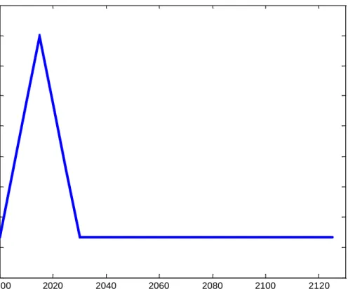
Figure 5: Labor Income Taxes across Different Cohorts at Different Time 20 30 40 50 60 70 80 0.05 0.1 0.15 0.2 0.25 0.3 Age Period 2 Period 3 Final St.St.
The optimal labor income tax rate varies substantially across cohorts. In the final Steady State the optimal labor income tax schedule is concave and increasing as a function of age, up to the point at which individuals start receiving a pension. Upon retirement the taxation of labor income (remember that retirement pensions are taxed at the same rate as regular labor income) is higher. This feature reflects the tension between the incentives for the fiscal authority to tax away the retirement pensions and the distortions that introduces on labor supply.
Intuitively, the fiscal authority introduces such labor income tax progressivity in order to undo the intergenerational redistribution in favor of the older cohorts that the social security system is generating.
As a result of this new structure of labor income taxation, individuals will provide very little labor supply after age 65 and almost none in the last period, as shown in Figure 6.
Figure 6: Labor Supply across Different Cohorts at Different Time 25 30 35 40 45 50 55 60 65 70 75 0 0.05 0.1 0.15 0.2 0.25 0.3 0.35 0.4 0.45 Age Initial St.St. Period 1 Final St.St.
Notice that the shape of labor supply is not dramatically changed with the reform, except for the fact that individuals would still provide some labor while receiving a retirement pension. However, the amount of labor supplied by the oldest cohorts is quite small.
The initial tax cuts, together with the increasing financial needs to finance the retirement pensions, necessarily imply that government debt has to increase in the initial periods following the reform.
Next, Figure 7 displays the evolution of government debt over GDP associated to the optimal reform.
Figure 7: Evolution of Debt to GDP Ratio 2000 2020 2040 2060 2080 2100 2120 0.45 0.5 0.55 0.6 0.65 0.7 0.75 0.8 Year
In order to finance retirement pensions debt would increase up to 77% of annual GDP (relative to its initial 50%). Later on this debt will be progressively repaid.
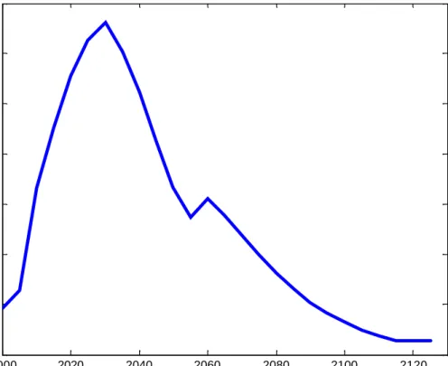
Overall, such a reform only generates welfare gains for those cohorts born once the demographic shock is over. However, the optimal response guarantees that the cohorts initially alive and those born during the shock enjoy the same level of utility as in the benchmark economy. Notice that by construction the initial old were not included in the objective function, and as a consequence the constraint to achieve at least the same utility level as in the benchmark economy has to be necessarily binding. Yet, this was not the case for new generations born during the demographic shock since they were included in the objective function of the fiscal authority. Yet, the optimal policy response implies that the constraint will be binding, and only after the demographic shock is over will newborn cohorts start enjoying higher welfare. The welfare gains accruing to newborns are plotted in Figure 8.
Figure 8: Welfare Gains of Newborn Generations 20001 2020 2040 2060 2080 2100 2120 1.02 1.04 1.06 1.08 1.1 1.12 1.14 1.16 Year Planner Ramsey
The optimal response associated to the sustainable policy contrasts with the findings where policies are exogenously specified as in De Nardi et al. (1999), where the initial cohorts are worse-off, and Jeske (2003) where the baby boomers and the grandchildren of the baby boomers suffer welfare losses. In our economy the cost of the shock is distributed over the cohorts initially alive or born during the shock. Different weights in the social welfare function would imply a different distribution of welfare gains across current and future generations.
Notice that the welfare gains associated to the reform just discussed, labeled as “Ramsey” in Figure 8, are much smaller than those associated to the First Best allocation, labeled as “Planner”.
Remember the discussion in Section 4. By construction we have prevented the fiscal authority from lump-sum taxing the retirement pensions. If we were to allow the fiscal authority to tax differently retirement pensions from regular labor income, the fiscal authority would choose to do so imposing on pensions taxes higher than a 100% effectively replicating a system with lump-sum taxes. Notice that the welfare gains from doing so (labeled as “Planner”) would be much higher, especially for the initial
This comparison indicates that the welfare costs of having to use distortionary taxation are very high, especially at the initial periods of the reform.
6. Conclusions
In this paper we have provided an answer to a very simple and policy relevant question: what should be the optimal response to a demographic shock? In order to answer this question we use optimal fiscal policy to determine the optimal way to finance some promised level of retirement pensions through distortionary taxation. In our experiment, the presence of a demographic shock renders the actual way of financing the social security system unsustainable and our approach endogenously determines how to accommodate this shock.
We find that the government can design a Pareto improving reform that exhibits sizeable welfare gains. Yet, the welfare gains will be concentrated for generations born in the distant future after the demographic shock is over. Our approach explicitly provides quantitative policy prescriptions towards the policy design of future and maybe unavoidable social security reforms.
The optimal response consists of the elimination of compulsory retirement, decreasing labor income taxation of the young and a temporary increase of government debt in order to accommodate the higher financial needs generated by the increase in the dependency ratio.
7. References
Atkinson, A.B. and J. Stiglitz (1980), Lectures in Public Economics, McGraw-Hill, New York.
Boldrin, M. and A. Rustichini (2000), “Political Equilibria with Social Security”,
Review of Economic Dynamics 3(1), 41-78.
Boldrin, M. and A. Montes (2004), “The Intergenerational State: Education and Pensions”, Federal Reserve Bank of Minneapolis Staff Report 336.
Chari, V.V. and P.J. Kehoe (1999), “Optimal Fiscal and Monetary Policy”, in J.B. Taylor and M. Woodford, eds., Handbook of Macroeconomics, Vol. 1C. Elsevier
Science, North-Holland, 1671-1745.
Conesa, J.C. and C. Garriga (2004), “Optimal Design of Social Security Reforms”, mimeo.
Cooley, T.F. and J. Soares (1999), “A Positive Theory of Social Security Based on Reputation”, Journal of Political Economy 107(1), 135-160.
De Nardi, M., S. Imrohoroglu and T.J. Sargent (1999), “Projected U.S. Demographics and Social Security”, Review of Economic Dynamics 2(3), 576-615.
Diamond, P. (1965), “National Debt in a Neoclassical Growth Model”, American Economic Review 55(5), 1126-1150.
Erosa, A. and M. Gervais (2002), “Optimal Taxation in Life-Cycle Economies”,
Journal of Economic Theory 105(2), 338-369.
Escolano, J. (1992), “Optimal Taxation in Overlapping Generations Models”, mimeo. Feldstein, M. and J.B. Liebman (2002), “Social Security”, in Auerbach, A.J. and M. Feldstein (eds.) Handbook of Public Economics, vol. 4, 2245-2324. Amsterdam, London and New York: Elsevier Science, North-Holland.
Gale, D. (1973), “Pure Exchange Equilibrium of Dynamic Economic Models”, Journal of Economic Theory 6(1), 12-36.
Garriga, C. (1999), “Optimal Fiscal Policy in Overlapping Generations Models”, mimeo.
Gollin, D. (2002), “Getting Income Shares Right”, Journal of Political Economy
110(2), 458-474.
Grossman, Gene M. and E. Helpman (1998), “Integenerational Redistribution with Short-Lived Governments,” Economic Journal 108(450), 1299-1329.
Hansen, G.D. (1993), “The Cyclical and Secular Behaviour of the Labour Input: Comparing Efficency Units and Hours Worked”, Journal of Applied Econometrics 8(1), 71-80.
Jeske, K. (2003), “Pension Systems and Aggregate Shocks”, Federal Reserve Bank of Atlanta Economic Review 88(1), 15-31.
Mendoza, E., A. Razin and L.L. Tesar (1994), “Effective Tax Rates in Macroeconomics: Cross-Country Estimates of Tax Rates on Factor Incomes and Consumption”, Journal of Monetary Economics 34(3), 297-323.
CESifo Working Paper Series
(for full list see www.cesifo.de)
___________________________________________________________________________ 1329 Chiona Balfoussia and Mike Wickens, Macroeconomic Sources of Risk in the Term
Structure, November 2004
1330 Ludger Wößmann, The Effect Heterogeneity of Central Exams: Evidence from TIMSS, TIMSS-Repeat and PISA, November 2004
1331 M. Hashem Pesaran, Estimation and Inference in Large Heterogeneous Panels with a Multifactor Error Structure, November 2004
1332 Maarten C. W. Janssen, José Luis Moraga-González and Matthijs R. Wildenbeest, A Note on Costly Sequential Search and Oligopoly Pricing, November 2004
1333 Martin Peitz and Patrick Waelbroeck, An Economist’s Guide to Digital Music, November 2004
1335 Lutz Hendricks, Why Does Educational Attainment Differ Across U.S. States?, November 2004
1336 Jay Pil Choi, Antitrust Analysis of Tying Arrangements, November 2004
1337 Rafael Lalive, Jan C. van Ours and Josef Zweimueller, How Changes in Financial Incentives Affect the Duration of Unemployment, November 2004
1338 Robert Woods, Fiscal Stabilisation and EMU, November 2004
1339 Rainald Borck and Matthias Wrede, Political Economy of Commuting Subsidies, November 2004
1340 Marcel Gérard, Combining Dutch Presumptive Capital Income Tax and US Qualified Intermediaries to Set Forth a New System of International Savings Taxation, November 2004
1341 Bruno S. Frey, Simon Luechinger and Alois Stutzer, Calculating Tragedy: Assessing the Costs of Terrorism, November 2004
1342 Johannes Becker and Clemens Fuest, A Backward Looking Measure of the Effective Marginal Tax Burden on Investment, November 2004
1343 Heikki Kauppi, Erkki Koskela and Rune Stenbacka, Equilibrium Unemployment and Capital Intensity Under Product and Labor Market Imperfections, November 2004 1344 Helge Berger and Till Müller, How Should Large and Small Countries Be Represented
in a Currency Union?, November 2004
1346 Wolfgang Eggert and Martin Kolmar, Contests with Size Effects, December 2004
1347 Stefan Napel and Mika Widgrén, The Inter-Institutional Distribution of Power in EU Codecision, December 2004
1348 Yin-Wong Cheung and Ulf G. Erlandsson, Exchange Rates and Markov Switching Dynamics, December 2004
1349 Hartmut Egger and Peter Egger, Outsourcing and Trade in a Spatial World, December 2004
1350 Paul Belleflamme and Pierre M. Picard, Piracy and Competition, December 2004 1351 Jon Strand, Public-Good Valuation and Intrafamily Allocation, December 2004
1352 Michael Berlemann, Marcus Dittrich and Gunther Markwardt, The Value of Non-Binding Announcements in Public Goods Experiments: Some Theory and Experimental Evidence, December 2004
1353 Camille Cornand and Frank Heinemann, Optimal Degree of Public Information Dissemination, December 2004
1354 Matteo Governatori and Sylvester Eijffinger, Fiscal and Monetary Interaction: The Role of Asymmetries of the Stability and Growth Pact in EMU, December 2004
1355 Fred Ramb and Alfons J. Weichenrieder, Taxes and the Financial Structure of German Inward FDI, December 2004
1356 José Luis Moraga-González and Jean-Marie Viaene, Dumping in Developing and Transition Economies, December 2004
1357 Peter Friedrich, Anita Kaltschütz and Chang Woon Nam, Significance and Determination of Fees for Municipal Finance, December 2004
1358 M. Hashem Pesaran and Paolo Zaffaroni, Model Averaging and Value-at-Risk Based Evaluation of Large Multi Asset Volatility Models for Risk Management, December 2004
1359 Fwu-Ranq Chang, Optimal Growth and Impatience: A Phase Diagram Analysis, December 2004
1360 Elise S. Brezis and François Crouzet, The Role of Higher Education Institutions: Recruitment of Elites and Economic Growth, December 2004
1361 B. Gabriela Mundaca and Jon Strand, A Risk Allocation Approach to Optimal Exchange Rate Policy, December 2004
1363 Jerome L. Stein, Optimal Debt and Equilibrium Exchange Rates in a Stochastic Environment: an Overview, December 2004
1364 Frank Heinemann, Rosemarie Nagel and Peter Ockenfels, Measuring Strategic Uncertainty in Coordination Games, December 2004
1365 José Luis Moraga-González and Jean-Marie Viaene, Anti-Dumping, Intra-Industry Trade and Quality Reversals, December 2004
1366 Harry Grubert, Tax Credits, Source Rules, Trade and Electronic Commerce: Behavioral Margins and the Design of International Tax Systems, December 2004
1367 Hans-Werner Sinn, EU Enlargement, Migration and the New Constitution, December 2004
1368 Josef Falkinger, Noncooperative Support of Public Norm Enforcement in Large Societies, December 2004
1369 Panu Poutvaara, Public Education in an Integrated Europe: Studying to Migrate and Teaching to Stay?, December 2004
1370 András Simonovits, Designing Benefit Rules for Flexible Retirement with or without Redistribution, December 2004
1371 Antonis Adam, Macroeconomic Effects of Social Security Privatization in a Small Unionized Economy, December 2004
1372 Andrew Hughes Hallett, Post-Thatcher Fiscal Strategies in the U.K.: An Interpretation, December 2004
1373 Hendrik Hakenes and Martin Peitz, Umbrella Branding and the Provision of Quality, December 2004
1374 Sascha O. Becker, Karolina Ekholm, Robert Jäckle and Marc-Andreas Mündler, Location Choice and Employment Decisions: A Comparison of German and Swedish Multinationals, January 2005
1375 Christian Gollier, The Consumption-Based Determinants of the Term Structure of Discount Rates, January 2005
1376 Giovanni Di Bartolomeo, Jacob Engwerda, Joseph Plasmans, Bas van Aarle and Tomasz Michalak, Macroeconomic Stabilization Policies in the EMU: Spillovers, Asymmetries, and Institutions, January 2005
1377 Luis H. R. Alvarez and Erkki Koskela, Progressive Taxation and Irreversible Investment under Uncertainty, January 2005
1378 Theodore C. Bergstrom and John L. Hartman, Demographics and the Political Sustainability of Pay-as-you-go Social Security, January 2005
1379 Bruno S. Frey and Margit Osterloh, Yes, Managers Should Be Paid Like Bureaucrats, January 2005
1380 Oliver Hülsewig, Eric Mayer and Timo Wollmershäuser, Bank Loan Supply and Monetary Policy Transmission in Germany: An Assessment Based on Matching Impulse Responses, January 2005
1381 Alessandro Balestrino and Umberto Galmarini, On the Redistributive Properties of Presumptive Taxation, January 2005
1382 Christian Gollier, Optimal Illusions and Decisions under Risk, January 2005
1383 Daniel Mejía and Marc St-Pierre, Unequal Opportunities and Human Capital Formation, January 2005
1384 Luis H. R. Alvarez and Erkki Koskela, Optimal Harvesting under Resource Stock and Price Uncertainty, January 2005
1385 Ruslan Lukach, Peter M. Kort and Joseph Plasmans, Optimal R&D Investment Strategies with Quantity Competition under the Threat of Superior Entry, January 2005 1386 Alfred Greiner, Uwe Koeller and Willi Semmler, Testing Sustainability of German
Fiscal Policy. Evidence for the Period 1960 – 2003, January 2005
1387 Gebhard Kirchgässner and Tobias Schulz, Expected Closeness or Mobilisation: Why Do Voters Go to the Polls? Empirical Results for Switzerland, 1981 – 1999, January 2005
1388 Emanuele Bacchiocchi and Alessandro Missale, Managing Debt Stability, January 2005 1389 Assar Lindbeck and Dirk Niepelt, Improving the SGP: Taxes and Delegation rather than
Fines, January 2005
1390 James J. Heckman and Dimitriy V. Masterov, Skill Policies for Scotland, January 2005 1391 Emma Galli & Fabio Padovano, Sustainability and Determinants of Italian Public
Deficits before and after Maastricht, January 2005
1392 Angel de la Fuente and Juan Francisco Jimeno, The Private and Fiscal Returns to Schooling and the Effect of Public Policies on Private Incentives to Invest in Education: A General Framework and Some Results for the EU, January 2005
1393 Juan C. Conesa and Carlos Garriga, Optimal Response to a Demographic Shock, January 2005