The Challenge of Tonal Fan Noise Prediction for an Aircraft Engine
in Flight
Carolin Kissner
1), S´
ebastien Gu´
erin
1), Lars Enghardt
1), Henri Siller
1), Michael Pott-Pollenske
2) 1)German Aerospace Center (DLR), Institute of Propulsion Technology,
Engine Acoustics, M¨
uller-Breslau-Str. 8, 10623 Berlin, Germany.
2)
German Aerospace Center (DLR), Institute of Aerodynamics and Flow Technology,
Technical Acoustics, Lilienthalpl. 7, 38108 Braunschweig, Germany.
Summary
Expensive fly-over tests are needed to verify that noise certification standards are fulfilled. Currently, no nu-merical alternative exists to perform a holistic ”vir-tual fly-over” test. As a step towards enabling such evaluations in the future, the authors focus on an iso-lated noise source - the tonal rotor-stator-interaction (RSI) of the fan stage. A high-fidelity simulation rely-ing on a state-of-the-art yet computationally efficient method is performed for a V2527 aircraft engine in approach conditions. The computational domain in-cludes the noise generation in the fan stage, its prop-agation in the engine inlet and bypass duct, as well as its radiation into the far field. Installation effects due to bifurcations and struts in the duct, ESS (engine section stator), liners, and inflow distortions are not considered. Post-processing methods are introduced and applied to the numerical data to allow for a mean-ingful comparison of the results to microphone data recorded during fly-over experiments. In particular, great care is taken to quantify the numerical dissipa-tion of the simuladissipa-tion inside the nacelle and to enable a suitable correction of the numerical data. The nu-merical simulation cannot fully reproduce the experi-mental data indicating that its level of complexity is not yet sufficient. As there is no obvious cause for the mismatch, it would be necessary to incrementally increase the complexity of the simulation in order to pinpoint the most significant sources and effects.
1
Introduction
To ensure compliance with current noise regulations, new aircraft have to be acoustically certified with fly-over noise tests according to procedures defined in the Annex 16 to the Convention on International Civil Aviation - Environmental Protection, Vol. I - Air-craft Noise [1]. Noise standards have to be met at the operating points of approach, sideline, and cut-back. In the future, noise certification regulations will become even more stringent. A high-fidelity,
nu-merical alternative to expensive fly-over noise tests, which are typically performed in the last stages of development just before an aircraft enters into com-mercial service, could enhance the aircraft design pro-cess. During ”virtual fly-overs”, relevant noise sources could be identified and quantified.
Some numerical studies that investigate the air-frame noise of an aircraft in flight were recently conducted using a lattice Boltzmann flow simula-tion in combinasimula-tion with a Ffwocs Williams-Hawkings (FWH) noise propagation scheme [2, 3, 4, 5]. All simulations were conducted for a Gulfstream G550 in landing configuration and neglect the contribution of the engine entirely. Good agreement in terms of surface pressures and far field noise between simula-tion data and windtunnel or fly-over measurements was demonstrated. However, fly-over noise tests re-quired for certification are not limited to airframe noise. While the airframe noise is, in fact, more signif-icant during landing than during take-off, the engine noise is thought to be slightly dominant or of a sim-ilar magnitude [6]. Thus, there is currently no com-prehensive, numerical approach that can match the results of fly-over noise tests. In this paper, the au-thors chose a different approach for tackling the same problem. To allow for the use of ”virtual fly-overs” in the design phase, such computations would need to be as accurate as possible while not demanding excessive amounts of computational resources. Thus, the complexity of such a computation would ideally be reduced to only include the noise sources and ef-fects that have the most significant contribution at the certification points. As a first step towards pin-pointing the most significant noise sources and de-termining the required complexity to achieve such a reduced yet accurate prediction, the authors decided to investigate one significant noise source, namely the rotor-stator-interaction tones of the fan, using a state-of-the-art, computationally efficient simulation tech-nique. Tonal rotor-stator-interaction noise in the fan, which is produced by the interaction of rotor wakes with the downstream stator row, is a dominant en-gine noise source. The investigated aircraft
configu-ration is the DLR ATRA research aircraft, an Airbus A320-232 equipped with two V2527-A5 engines. This paper strives to answer the question if a simulation relying on state-of-the-art yet relatively economical techniques can reproduce the fan tones observed dur-ing a fly-over of this aircraft at approach conditions.
The high-fidelity Computational Fluid Dynamics (CFD) simulation used the Harmonic Balance tech-nique [7] and phase-shift, i.e. chorochronic, bound-ary conditions to simulate the tonal RSI noise for the fan of a full-scale V2527 engine. The computa-tion considers the noise generacomputa-tion mechanism within the fan stage, its propagation through the engine’s inlet and bypass duct, and its radiation to the far field. Lastly, the sound is radiated to observer po-sitions on the ground using a FWH integral method [8]. The approach was successfully used in the past by Holewa et al.[9] to assess the fan tones of a config-uration under test bed conditions. Transonic as well as subsonic operating points were assessed. For dom-inant modes, the simulation results differed by less than 3 dB from the measured data in the far field near the engine inlet and in the bypass duct. The ex-perimental modal spectra contained generally weak, additional azimuthal modes, which were not caused by the rotor-stator-interaction. Only at the inlet at subsonic, approach-like conditions, the RSI mode was poorly radiated in the simulation and in the noise test. The experimental data was thus dominated by the ad-ditional modes and the sound pressure levels in the forward arc were underestimated in the simulation.
To allow for a meaningful comparison of the nu-merically determined tonal fan noise to the fan tones extracted from experimental data of a fly-over, the application of suitable post-processing techniques for both numerical and experimental data is essential. A particular focus of this paper will be the post-processing of the numerical results. Correction pro-cedures to account for numerical dissipation in the simulation were developed and applied. In addition, the numerical data was averaged over a range of direc-tivity angles to emulate the post-processing of exper-imental data. Lastly, an equivalent monopole source was determined so that the numerical directivity re-sembles the directivity typically observed in fly-over experiments.
This paper will be structured as follows: At first, the fly-over measurements will be discussed includ-ing a description of the two different experimental se-tups and of the post-processing applied to the mea-sured data. The setup of the numerical simulation and mesh generation procedure will be explained next. A focus of this paper will be the extraction and post-processing of the numerical data, which will be dis-cussed in a separate section. Lastly, the numerical data will be compared to the experimental data at the first three blade passing frequencies (BPF’s) and the results will be discussed.
Table 1: Overview of flight conditions rot. flap/ land- true speed slat ing
air-N1 [%] angles gear speed [kts]
Num. 53.42 - - 133 Exp. A 50.9 27◦/40◦ down 139 Exp. B 53.0 22◦/20◦ up 160 - 165 flight path B A
Figure 1: Sketch of experimental setups. Elliptical array denoted by letter A. Linear array denoted by letter B.
2
Fly-over measurements
Fly-over measurements were performed by two differ-ent groups of researchers, each using a differdiffer-ent exper-imental setup. The two different experexper-imental setups and their respective data will hereafter be denoted by experiment A andexperiment B. To get a more com-plete description, the authors chose the flights in each experimental data set, that most closely matched the numerical operating conditions in terms of rotational speed and true airspeed (see Table 1). The numer-ically imposed operating conditions during approach were determined using a performance cycle model de-fined by Wolters et al. [10]. It should, however, be noted that the deployment angles of the high lift de-vices and landing gear settings differ between experi-ments A and B.
In the following subsections, the experimental se-tups of experiments A and B as well as the post-processing of their respective data sets are briefly de-scribed.
2.1
Description of experimental
se-tups
Two teams of researchers conducted fly-over measure-ments on DLR’s Advanced Technology Research Air-craft (ATRA). Both teams, whose experiments are de-noted by letters A and B, used different experimental setups.
positioned slightly starboard of the flight path in or-der to avoid the symmetry plane of the aircraft, as can be seen in Figure 1. The array contained 248 electret microphones and covered an area of 43 m by 36 m. The longer axis was oriented parallel to the direction of flight in order to increase the resolution to enable the use of beamforming for source localization. Only one fly-over was recorded at the specified operating conditions. More details regarding the experimental setup can be found in Siller et al. [11, 12].
For experiment B, a linear microphone array was positioned perpendicular to the flight path (see Figure 1). The array consisted of nine microphones mounted on the ground. A similar setup was used by Pott-Pollenske et al. [13] for studying a different aircraft configuration. Only the three center microphones of the array, that were positioned either directly or nearly underneath the flight path, were considered for the analyses presented here. Due to the greater dis-tance from the outer microphones to the noise source, the narrow band spectra are dominated by the cor-rection for the atmospheric absorption at frequencies of interest for the extraction of fan tones, i.e. at fre-quencies close to or lower than the third harmonic of the blade passing frequency. The comparatively low number of microphones that could be used for aver-aging the spectra was partly offset by the fact that data for nine, almost identical flights were provided. Thus, spectra at the different positions were averaged over the number of flights before averaging the spectra over the number of microphones. Therefore, a higher statistical precision could be reached.
2.2
Post-processing
of
experimental
data
The microphone signals were corrected in the time do-main to remove the frequency shift due to the Doppler effect. Then, the tones and respective background noise levels were extracted at the harmonics of the blade passing frequency.
All narrow band spectra were adjusted to remove the atmospheric absorption according to ISO stan-dard 9613-1 [14], which is based on the modeling of molecular phenomena to derive analytical expressions for the atmospheric attenuation as introduced by Bass et al. [15]. An overcompensation of the sound pressure levels at high frequencies occurs when the spectral levels meet the noise floor. Thus, the measured levels remain approximately constant, while the corrected levels increase with an increasing frequency.
Further corrections were introduced to enable a comparison with the numerical data. All experimen-tal spectra were corrected to account for the discrep-ancy in rotational speed ∆N compared to the
numer-ical settings using a scaling law derived from
Heid-mann and Feiler’s work [16]: ∆N = 50 log10 N num Nexp . (1)
Here,Nnum is the rotational speed of the simulation,
whileNexpdenotes the rotational speed of the
exper-iments. For experiment A, ∆N is equal to 1.05 dB.
For experiment B, ∆N is equal to 0.17 dB. It should
be noted that Equation 1 agrees with a non-compact dipole-like source characteristic, which is reasonable for the rotor-stator-interaction tones of a fan but not necessarily for other broadband noise sources of an aircraft in flight. In addition, numerical and exper-imental far field data had to be normalized to the same observer distance. An observer radius of 100 m was chosen for the analysis of the numerical data. A correction ∆R for the experimental data can be
de-termined by ∆R= 20 log10 R num Rexp , (2)
whereRnum denotes the numerical observer distance
andRexp, the experimental observer distance.
In the end, the authors aim to compare the sound pressure levels as a function of the directivity an-gles for the first three harmonics of the BPF. The directivity angles are defined so that θ = 0◦
corre-sponds to the observer position in the forward arc upstream of the aircraft. Conversely, a directivity an-gle of θ = 180◦ corresponds to the observer position
in the rear arc downstream of the aircraft. The tones along with the respective background noise levels were extracted from the given narrow band spectra. Since the fan tones are scattered over several frequencies, the absolute sound pressure levels were determined by a summation over the respective bands and several of their neighboring bands. The background noise level was extracted at the bottom of the tonal peaks. The results are shown in Figure 2. It should be noted that some tones could not be identified in the spec-tra, particularly at higher frequencies and at increas-ing directivity angles. The dominant tone occurs at the 1st harmonic of the BPF. The tones at the higher harmonics are only slightly lower in amplitude. The amplitudes of the sound pressure levels of tones and background noise do not vary much with respect to the directivity angle. Therefore, a tendency towards a monopole-like directivity can be observed.
The differences in data of experiments A and B shall not be discussed in detail as such a discussion is out-side the scope of this paper. It is expected that most of the observed differences are due to different settings of the high-lift devices, different pitch angles, and due to the landing gear (see Table 1). It should also be noted that there are some uncertainties regarding the experimental data. For some microphones, wooden tiles were placed under the microphones, which could
0◦ 45◦ 90◦ 135◦ 180◦ SPL [10 dB/div.] tones A broadband A tones B broadband B (a) 0◦ 45◦ 90◦ 135◦ 180◦ SPL [10 dB/div.] tones A broadband A tones B broadband B (b) 0◦ 45◦ 90◦ 135◦ 180◦ SPL [10 dB/div.] tones A broadband A tones B broadband B (c)
Figure 2: Experimentally determined directivity of tonal and background noise at a) BPF 1, b) BPF 2, and c) BPF 3.
lead to refraction effects. The error should be within 1 to 2 dB. In addition, some difficulties were encoun-tered at this flight condition while determining the flight path using a combination of laser distance me-ters and Global Navigation Satellite System (GNSS) data from the aircraft. This could lead to small errors in de-Dopplerizing the spectra. Nonetheless, errors are expected to be smaller than 1 dB.
3
Numerical simulation
In the following section, the numerical setup will be introduced and the used mesh generation procedure will be outlined.
3.1
Setup
The in-house CFD solver for internal flows, TRACE [17], was used to simulate the tonal fan noise of the V2527 engine at approach. The turbulence was mod-eled with the Menter SST k −ω model [18] and the spatial discretization was done via a Monotonic Upstream Scheme for Conservation Laws (MUSCL) approach [19] of second order accuracy based on Fromm’s scheme. The main emphasis in setting up this simulation was to accurately predict the tonal fan noise as efficiently as possible. Therefore, the Har-monic Balance (HB) technique [7] and a phase-shift boundary condition [20] were applied.
The HB technique is a non-linear approach, which solves the unsteady Reynolds Averaged Navier-Stokes (uRANS) equations in the frequency domain rather than in the time domain. The main advantage is that this tends to be more efficient, especially when solu-tions are only needed at blade passing frequencies as is the case in the paper. In fact, both Frey et al. [21] and Holewa et al. [22] have shown that a HB simula-tion runs faster than a tradisimula-tional uRANS simulasimula-tion. Frey et al. [21] simulated the tonal fan noise of DLR’s Ultra High Bypass Ratio (UHBR) at the second blade passing frequency in approach conditions. In addition to its computational efficiency, the authors were able to prove that the HB results match well with uRANS and experimental results. Holewa et al. [22] used the approach to study the impact of the interaction of steady hot streaks with a high-pressure turbine stage on the overall tonal noise. They were able to show that the HB simulation, which was designed to re-solve harmonics 1 and 2 of the BPF, ran 20 times faster than the uRANS simulation. It was addition-ally observed that the phase-shift boundary condition and the non-reflecting in- and outflow boundary con-ditions are more robust in combination with the HB technique leading to an accelerated convergence.
The phase-shift boundary condition exploits the ro-tational symmetry of the blade rows in turbomachin-ery. For this simulation, the fan stage was reduced to single-passage rotor, outlet guide vane (OGV), and
(a)
(b)
Figure 3: Complexity of engine configuration, which includes a) a spliced liner and a P2T2 sensor in the en-gine inlet and b) struts and bifurcations in the bypass duct (photos courtesy of Lech Modrzejewski, 2013).
engine section stator (ESS) blocks. While included in the simulation, the ESS was only considered for com-puting the mean flow. The implication of neglecting the ESS as a potentially relevant acoustic source in the simulation is included in the discussion section as one possible explanation for the discrepancy between the experimental and numerical data.
The phase-shift boundary condition was also ap-plied in the engine inlet, bypass duct, and far field allowing for a reduction of the computational domain to two cells in the circumferential direction. The com-plex engine configuration, which is illustrated in Fig-ure 3 was simplified to facilitate such a reduced, rota-tionally symmetric domain. The drooped inlet, bifur-cations and struts in the bypass duct, the P2T2 probe and spliced liner in the inlet duct were not accounted for. As the inflow distortion due to the incidence an-gle of the nacelle decreases almost exponentially in the inlet section of an engine at moderate angle of attack [23], it was assumed that its impact as a new source of sound can be neglected. This assumption as
well as other relevant assumptions are reconsidered in the discussion section in light of this paper’s results and in the context of other recent studies. To prevent any flow detachment at the positions of the installa-tions in the duct, the bypass geometry was slightly modified to keep the area of the duct constant in that section. Any acoustic liners and the engine core were also not included in the simulation.
3.2
Mesh generation
The mesh of a numerical simulation is always a com-promise between accuracy and cost. A fine mesh reduces numerical dispersion and dissipation effects but is costly in terms of computational resources. A coarser mesh will be cheaper but result in a loss in ac-curacy. For this simulation, the authors pursued the following strategy: A best practice procedure, which was previously described by Kissner et al. [24], was applied with the aim of resolving the RSI tones with at least 40 points per wavelength (PPW) for 2nd har-monic of the BPF. This resulted in a resolution of at least 30 PPW for 3rd of the BPF. Instead of doing a mesh study, numerical dissipation was quantified and used to correct the resulting far field noise data ac-cordingly (see Subsection 4.2).
The current best practice for generating structured meshes is loosely based on the findings of Schnell [20], who performed an in-depth study of dissipation and dispersion effects for a two-dimensional test case. He determined that a mesh resolution of 20 to 25 points per wavelength (PPW) resulted in a dissipation rate of 0.5 dB per wavelength perpendicular to the wave-front. However, a two-dimensional test case is not di-rectly comparable to a fan stage. The Mach number and mesh resolution are not constant. In addition, a measure based on the wavefront is not practical as a wavefront changes depending on the mode and its po-sition in the duct. To account for these uncertainties, an established practice is to aim for 40 PPW in all directions for the acoustically cut-on modes. This is conservative compared to other meshing routines used by different authors [25, 26, 27] in the community, who typically aim for a resolution of at least 20 to 25 PPW. Thus, the configuration studied in this work is comparatively rather well resolved. Nonetheless, nu-merical dissipation still occurs and accumulates due to the sheer size of the acoustically resolved domain, which not only includes the fan stage itself but also the entire bypass duct and portions of the far field. It is thus useful to analyze and quantify the dissipation in order to correct numerical results (see Subsection 4.2).
To design a suitable mesh for studying tonal fan noise, it is essential to know which acoustic modes are relevant. Acoustic, azimuthal modes resulting from RSI must fulfill the Tyler-Sofrin rule [28]
Table 2: Cut-on RSI modes
harmonic h / azimuthal radial mode frequency f [Hz] mode order m order n
1 / 1107 -
-2 / -2-213 -16 0-3
3 / 3320 6 0-3 (bypass) 0-13 (inlet)
where m describes the azimuthal mode order and k
represents an integer value. The harmonic of the BPF, which can be determined by multiplying the ro-tational speed of the rotor Ω with the number of rotor fan bladesB(BP F =B·Ω), is denoted byh. For this configuration, the number of rotor fan bladesB is 22 and the number of stator fan bladesV is 60. In the next step, it has to be analyzed, which of the deter-mined Tyler-Sofrin modes are cut-on in the duct. The results are listed in Table 2. No modes are cut-on at BPF 1, while one azimuthal mode is cut-on at BPF’s 2 and 3. A positive azimuthal mode order means that the mode rotates in the same direction as the rotor and vice versa. More radial modes are relevant in the inlet than in the bypass duct, since the duct area is larger in the inlet.
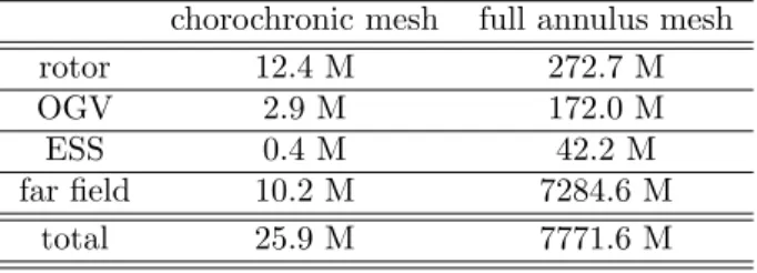
In order to achieve the desired resolution of 40 PPW in all directions at harmonic 2, the following approach was used: The wavelength in the axial direction was analytically determined at a position up- and down-stream of the fan stage respectively in order to find the maximum cell size in axial direction. The mesh resolution in azimuthal direction was - in this case - dictated by aerodynamic rather than acoustic con-siderations, since resolving boundary layers and vis-cous wakes yields in more circumferential cells than would be required to resolve the relatively small az-imuthal mode orders. In the radial direction, modes of a low radial order tend to be most energetic close to the tip radius. Thus, a clustering of the radial grid points near the tip radius is desirable. The radial grid resolution was chosen to be similar to compara-ble simulations and to avoid high cell aspect ratios, i.e. cells should have similar side lengths in all di-rections. The cells in the far field were designed to have approximately the same size as the cells within the duct in acoustically resolved regions. In regions near the boundaries of the far field, a cell stretching was introduced to suppress reflections at the far field boundary condition. The entire far field domain mea-sures about 16.6 fan diameters in the axial direction and about 2.5 fan diameters in the radial direction. The acoustically resolved far field region begins more than two fan diameters upstream of the engine in-let and ends over five fan diameters downstream of the engine outlet. The resulting mesh contains about 25.9 million cells. The largest blocks are the rotor and
Table 3: Number of cells of used, chorochronic mesh and of an equivalent, full annulus mesh
chorochronic mesh full annulus mesh
rotor 12.4 M 272.7 M
OGV 2.9 M 172.0 M
ESS 0.4 M 42.2 M
far field 10.2 M 7284.6 M
total 25.9 M 7771.6 M
far field blocks, each containing more than 10 million cells. Without the chorochronic boundary condition, a mesh of an equivalent resolution would contain over 7.7 billion cells (see Table 3), featuring 500 millions in the fan stage alone. On the one hand, this illus-trates the fine mesh resolution of this setup. On the other hand, a simulation using an equivalent mesh spanning the full annular duct would have been im-possible to perform on the current computing infras-tructure. The used mesh resolution and the size of the computational domain would have had to be signifi-cantly reduced both in the zone of the fan stage and in the far field. The simplification of the configura-tion to rotaconfigura-tionally symmetric computaconfigura-tional domain is thusa prioria sensible choice to drastically reduce the computational time.
4
Post-processing of numerical
data
To allow for a comparison of the numerically deter-mined and measured fan tones, the numerical data had to be extracted in the far field and to be cor-rected to account for numerical dissipation effects and the total number of engines. In addition, the nu-merical data was processed to emulate the post-processing and the characteristic, monopole-like di-rectivity of the experimental data.
4.1
Determination of far field
directiv-ity
To investigate far field noise, the FWH method based on the work of Weckm¨uller et al. [8] was applied. In order to receive reasonable results, the choice and po-sitioning of the FWH integration surfaces, where the pressure perturbations are extracted and propagated to the observer positions, is essential. The FWH ap-proach assumes constant mean flow at the position of the integration surfaces and in order to capture all of the emitted sound, the surface should enclose the sound source. These aims are easily met near the inlet of the engine but prove to be a challenge near the outlet of the engine. A closed integration surface would cut through the shear layer between ambient air
(a)
(b)
(c)
Figure 4: FWH integration surfaces shown for a) mean flow, b) BPF2, c) and BPF3. The box signi-fies the rotating block, which contains all harmonics of the BPF.
and bypass flow and through the shear layer between the bypass and core flows. An open integration does not fully enclose the sound source and emitted sound could potentially be neglected. The authors chose the latter option in order to not violate the constant flow assumption of the FWH technique. In addition, a comparison of the two variants showed that the devi-ation in the overall sound power levels was less than 0.25 dB at BPF 2 and BPF 3 (see Kissner et al. [24]) with little differences in the directivity of the sound pressure. The FWH integration surfaces are shown in Figure 4. The 180 observer positions were placed in a semicircle of radius 100 m around the engine.
The FWH method outputs real pre and
imagi-nary fluctuating pressurespimat each sensor position,
which can be used to determine sound pressure levels:
SP L[dB] = 10·log10 p2rms p2 ref ! . (4)
The reference pressure prms is equal to 2·10−5 Pa.
The root mean square pressureprmsis determined by prms= r 2·(pre,in+pre,out)2 + (pim,in+pim,out)2 , (5)
where pre and pim are the real and imaginary part
of the Fourier coefficients of the complex pressure field for a two-sided spectrum, the subscript in
de-notes the contribution from the engine inlet, and the subscript out, the contribution from the engine
out-let. The resulting sound pressure levels are shown as
0◦ 45◦ 90◦ 135◦ 180◦ SPL [10 dB/div.] inlet outlet total (a) 0◦ 45◦ 90◦ 135◦ 180◦ SPL [10 dB/div.] inlet outlet total (b)
Figure 5: Numerically determined directivity of fan tones at a) BPF 2 and b) BPF 3.
a function of the directivity angle θ at harmonics 2 and 3 of the BPF in Figure 5. It can be seen that the overall noise emitted at BPF 2 is dominated by the emission at the engine outlet. At directivity an-gles near 40◦, the total sound pressure line becomes jagged. This can occur, if the sound pressure origi-nating from engine inlet and outlet are of a similar magnitude but have a different phase. At BPF 3, contributions from both inlet and outlet influence the overall directivity.
4.2
Consideration of numerical
dissi-pation
To analyze the numerical dissipation, the sound power was first determined at different positions in the duct to identify trends and observe insightful phenomena. In the second step, a correction was formulated and applied to the far field data.
To determine the sound power within the duct, the extended plane pressure mode matching technique of Wohlbrandt et al. [29] was used. The technique can distinguish between sound and unsteady fluctuating pressures with convective characteristics. It relies on the assumption of uniform flow and of slowly chang-ing duct contours. For the analysis with swirl, which
0
2
4
6
relative axial coordinate [-]
sou
n
d
p
ow
er
le
ve
l
[20
d
B
/d
iv
.]
BPF 2
BPF 3
Figure 6: Sound power levels in duct. Solid lines mark the sound waves emitted by the fan stage towards the duct ends. Reflections back to the fan stage are shown by dashed lines. The line markers indicate the propagation direction: ”+”-markers denote a propa-gation in positive, axial direction, i.e. downstream. ”-”-markers denote a propagation in negative, axial direction, i.e. upstream.
is present in the interstage, a solution for solid body swirl flows is applied. This mainly includes two ex-tensions: i) the description of the acoustic modal so-lution in rotating mean flows following Morfey [30], ii) the calculation of an equivalent solid body swirl flow with the same net force, mass flow, angular mo-mentum and enthalpy flow as the original CFD mean flow solution (method not published yet). Its acous-tic model cannot consider radial flow and the aero-dynamic model neglects the viscous dissipation of the perturbations and effects due to the wake expansion. The sound power levels in the duct are shown in Figure 6. In this figure, solid lines mark the prop-agated sound, while reflections are shown by dashed lines. The line markers indicate the propagation di-rection: ”+”-markers denote a propagation in posi-tive, axial direction, i.e. downstream. ”-”-markers denote a propagation in negative, axial direction, i.e. upstream. Particularly in the domains up- and down-stream of the fan stage, the sound power levels of re-flections are 10 to 35 dB smaller than prevalent sound power levels. This is to be expected for modes that are well cut-on. Furthermore, the main sound power levels decrease nearly linearly with an increasing dis-tance from the fan stage. Since the dissipation behav-ior is linear and nearly all dissipation in a duct can be attributed to numerical dissipation, it can be quanti-fied in terms of dissipation rates, which are listed in
Table 4: Dissipation rates in duct direction harmonic h dissipation rate
of BPF [dB per OGV radius]
2 upstream 0.5
downstream 1.0
3 upstream 2.2
downstream 1.2
Table 4. The dissipation rates are given as decrease in sound power per OGV radius as the usual definition in PPW is not practical due to the large number of modes. It can be observed that the dissipation rates are higher for BPF 3 than for BPF 2. This is reason-able as resolving higher frequencies requires a finer grid resolution.
The sound power levels in the interstage section of the duct are insightful as well. It proves that the sound originates at the stator vanes, since the sound power levels are higher in the upstream direction. Ro-tor shielding can also be clearly seen: as the sound originating from the OGV passes through the rotor row, its level drops off significantly. In addition, the decrease in sound power is about 10 dB larger for the BPF 2 than for the BPF 3. Two factors could con-tribute to such a shielding effect: Firstly, the swirl in the flow increases the tendency of an acoustic mode to become cut-off if the swirl Mach number and the cir-cumferential mode have the same rotational direction as shown by Roger and Arbey for simplified solid-body swirl and free vortex flows [31]. Those obser-vations were confirmed by e.g. Masson et al. [32] for realistic flows with swirl and shear. This described ef-fect could impact the azimuthal mode order 6 at BPF 3. Secondly, azimuthal modes rotating in the same di-rection as the rotor are transmitted more effectively as demonstrated by Kaji and Okazaki [33]. This lat-ter effect seems to be dominant here and explains why the shielding effect for mode -16 of BPF 2 is stronger than for mode 6 at BPF 3. The effects of the shield-ing effect can also be guessed from Figure 5, where the sound radiated from the inlet is less compared to the sound radiated from the engine outlet.
In the next step, a correction was formulated based on the previous findings regarding the numerical dissi-pation. The correction was applied to the fluctuating pressures used for computing the sound pressure lev-els:
prms=
r
2·(fin·pre,in+fout·pre,out)
2
+ (fin·pim,in+fout·pim,out)
2
,
(6)
fac-Table 5: Dissipation between fan stage and FWH sur-faces in PWL
dissipation [dB] At inlet At outlet BPF (h=2) 1.5 dB 4.5 dB BPF (h=3) 3.2 dB 7.0 dB
tors are applied. These are quantified as
fi= 10
∆diss,i
20 , (7)
where ∆diss,i denotes the difference in sound power
in decibels between the fan stage and the FWH inte-gration surface. The ∆diss,i - values for both BPF’s
at the in- and outlet of the engine are listed in Table 5. The correction equation and the definition of the correction factor make two inherent assumptions:
1. All dissipation is numerical dissipation.
2. The numerical dissipation has a linear behavior between the fan stage and the FWH integration surface.
Both assumptions are necessary simplifications of a more complex problem. Particularly near the outlet of the engines, not all dissipation will necessarily be numerical dissipation. Bechert [34] has shown that acoustic energy can be transformed into vortical en-ergy in shear flows. This effect - if relevant for this case - will be neglected by the introduced correction. The impact of the correction of the sound pressure levels can be seen in Figure 7. The correction has a greater effect in the rear of the engine than at the inlet because the bypass duct is longer than the inlet duct and thus more overall numerical dissipation is induced.
4.3
Correction for number of engines
As the ATRA aircraft has two engines and the simu-lation only considered one engine, the sound pressure has to be corrected accordingly by the correct number of enginesn: SP L[dB] = 10·log10 n· p2rms,total p2 ref ! . (8)
This correction assumes that both engines are uncor-related sound sources. In Figure 7, it can be seen that the correction causes an increase in the sound pressure levels of 3 dB.
4.4
Smoothing of data
The post-processing of fly-over measurements is more challenging than for static test beds or wind tun-nels since the source is in motion. Particularly at
0◦ 45◦ 90◦ 135◦ 180◦ SPL [10 dB/div.] initial + no diss. + 2 engines + smoothing monopole (a) 0◦ 45◦ 90◦ 135◦ 180◦ SPL [10 dB/div.] initial + no diss. + 2 engines + smoothing monopole (b)
Figure 7: Numerically determined directivity of RSI tones and corrections at a) BPF 2 and b) BPF 3. a directivity angle of 90◦, the available integration time reaches a minimum. To increase the statisti-cal accuracy, an averaging over range of directivity angles is needed. Thus, there is built-in smooth-ing of the directivity information, which results from the post-processing of the experimental data. To re-produce this smoothing effect, the numerically deter-mined sound pressure levels were smoothed by a con-volution with a Gaussian bell function over a range of directivity angles. The chosen range of angles was three degrees in both directions, which approx-imately corresponds to the range of angles used in post-processing the experimental data. The effect can be seen in Figure 7.
4.5
Determination of an equivalent
monopole
As previously shown in Figure 2, the experimental results display a monopole-like directivity behavior. In the numerical simulation, the directivity is pro-nounced and quite unlike a monopole. This
obser-vation is quite reasonable. The simulation considers pure rotor-stator-interaction noise, which is charac-terized by one relevant cut-on mode at BPF’s 2 and 3. When isolated fan noise is considered experimentally in fan test rigs, the modes are generally dominated by the RSI modes only as shown by Heidelberg [35] and Holewa et al. [9]. Scattering mechanisms at installa-tions within the duct like struts and bifurcainstalla-tions are neglected in the simulation. The interactions with installations would cause each mode to scatter into other modes. Whereas one single mode has a strong directivity, multiple modes - each having a strong but different directivity - result in a smoother directivity when added up. The more modes carry acoustic en-ergy, the more the directivity becomes a monopole. It is assumed here that the overall sound power is unaf-fected by the scattering. Since the experimental data includes scattering effects, thus explaining its direc-tivity characteristic, the numerical data does not. To emulate the experimental data, a monopole of equiv-alent sound power was determined for the numerical data. The sound power resulting from sound pressure
pwas calculated by the equation
P = Z
S
IinidS, (9)
whereni is the vector normal to the integration
sur-face,Ii, the acoustic intensity vector, and dS, the
el-emental surface. An ”equivalent” monopole has the same overall sound power. For small Mach numbers
M, the following expression can be applied to calcu-late the root mean square pressure, which is constant at all directivity angles:
prms' s P ρ0c0 4πR2 1 4M ln 1 + 2M 1−2M −1 ,∀M 1. (10) Here,ρ0is the static pressure andc0denotes the speed
of sound. R describes the distance of the observers to the sound source. The equivalent monopoles are shown in Figure 7.
5
Comparison of numerical and
experimental far field data
After applying corrections to the numerical data, a comparison of the numerically determined fan tones to the fan tones from the experiments is shown in Fig-ure 8. It should be noted that all shown sound pres-sure levels are absolute levels for both numerical and experimental data. All directivity plots use the same dB-scale and can therefore be directly compared.The difference between the numerical and mental data is most striking at BPF 1. In the experi-mental data, the fan tone at BPF 1 is cut-on and dom-inant. The simulation cannot reproduce this result as
0◦ 45◦ 90◦ 135◦ 180◦ SPL [10 dB/div.] tones A tones B numerical (a) 0◦ 45◦ 90◦ 135◦ 180◦ SPL [10 dB/div.] tones A tones B numerical monopole (b) 0◦ 45◦ 90◦ 135◦ 180◦ SPL [10 dB/div.] tones A tones B numerical monopole (c)
Figure 8: Comparison of numerically determined to measured RSI tones at a) BPF 1, b) BPF 2, and c) BPF 3.
it only considers rotor-stator-interaction tones. In ad-dition, the flow and the geometry are axisymmetric, thus eliminating the possibility of modal scattering, which would cause observed modes to differ from the Tyler and Sofrin’s rule. As a consequence, there are no cut-on RSI modes at BPF 1. The sound pres-sure detected in the simulation can be attributed to the low radiation effectivity of cut-off modes [36] and possibly to hydrodynamic perturbations originating in the wakes of the OGV and rotor blades. Thus, the strong mechanism that causes the fan tone at BPF 1 to be cut-on in the experiment is not included in the simulation.
As expected, the directivity patterns calculated nu-merically are characterized by the presence of pro-nounced lobes, which are typical if only few induct modes are contained in the radiated sound field. In contrast, the measured directivity is much smoother and, therefore, closer to a monopole-like behavior. While the amplitude of the sound pressure is compa-rable for the equivalent monopole and the experimen-tal data at the 2nd harmonic of the BPF, this is not the case at 3rd harmonic of the BPF. In the simula-tion, there is also a significant difference in the overall magnitude of the numerically determined sound pres-sure between BPF’s 2 and 3. This decrease is less pronounced in the measurements.
It can be concluded that the simulation is not yet adequate in terms of its complexity for accurately predicting the fan tones, in particular the directivity shapes, of a V2527 engine in flight.
Some effects that could potentially explain the dis-crepancies between the experimental and numerical fan tones include:
• Installation effects within the duct due to struts and bifurcations are not considered in the simu-lation. Research by Holewa et al. [37] and by Re-donnet and Druon [38] suggest that bifurcations and struts cause a richer modal content of the RSI tones due to several mechanisms: i) sound generation by the rotor wake (vortical) interac-tion with those structural elements, ii) scatter-ing of the acoustic waves into new modes as they propagate through obstacles, and iii) impact of the potential field of the bifurcations on the ro-tor wake structure before they interact with the stator. This can not only jeopardize a cut-off fan design as shown by Winkler et al. [39] but also result in a smoother directivity in the far field. In fact, the acoustic scattering at the by-pass bifurcations suffices to significantly change the far field directivity as observed by Chen et al. [40]. They found that the directivity was less pro-nounced and the sound pressure levels increased by some decibels at some directivity angles com-pared to a simulation neglecting bifurcations. An increase in sound power due to an interaction of the rotor wakes with duct obstacles also depends
on the separation distance.
• Only the fan tones resulting from the interac-tion of the rotor wakes with the fan OGV’s was considered, whereas the contribution of the ESS was neglected. Results in the literature are not conclusive regarding the importance of the ESS contribution to the overall tonal fan noise, which lead to the hypothesis that the fan design and the applied operating conditions play a key role. Thus Holewa et al. [9] showed that the rotor-ESS-interaction tones were significantly smaller than the rotor-stator-interaction tones, despite the fact that the ESS is twice closer to the ro-tor than the OGVs. Winkler and al. [39] also made similar observations. Contradictorily, the results presented by Namgoong and Arisetti [41] show the presence of a strong acoustic field pro-duced by the ESS at 2nd harmonic BPF, which propagates up into the bypass duct.
• Inflow distortions due to the incidence angle are not included in the simulation. The work of Gu´erin and Holewa [42] suggests that this effect is less important than others. Gu´erin and Holewa numerically investigated an inflow distortion due to a typical incidence angle at approach for a full annulus fan stage featuring a drooped inlet. They observed only a marginally higher acoustic power level compared to a simulation with a clean in-flow. However, the SPL directivity was impacted by the distortion in the forward arc due to the asymmetric flow gradients at the inlet. Contrar-ily to that, the work done by Daroukh et al. [27] shows that the emitted sound of an engine con-sidering an asymmetric intake can significantly increase - in their case by about 3 dB compared to an equivalent setup considering an axisymmet-ric intake. Also, the P2T2 sensor could create a tone by the interaction of its wake with the rotor.
• Liners are neglected in the computation. Even though liners exist to damp emitted acoustic waves, they can also have a negative impact on the noise emission if they are badly designed. Thus, the interaction of the rotating pressure field with liner splices in the duct inlet can cause energy to be transferred from non-propagating, rotor-locked pressure field modes into lower, cut-on mode orders as discussed in the works of McAlpine and Wright [43] and Bassetti et al. [44]. Furthermore, liners are known to modify the directivity of the acoustic field radiated through the inlet [45] or the nozzle [46]. The degree of impact depends on the wave and liner character-istics.
• Another factor, which was not considered in the simulation, is that the engines of the ATRA re-search aircraft have been in service for many
years. A degradation of the engine liners and changes of the engine geometry - particularly of the blade geometry - due to wear and mainte-nance work can alter the noise signature of an engine. In fact, acoustic methods for the detec-tion of blade faults in turbomachinery [47, 48] analyze the altered sound emission by comparing it to a ”healthy” configuration.
This list is not meant to be exhaustive but rather to emphasize the complexity of the problem at hand. Only future investigations can shed light onto impor-tant effects and sources, which need to be considered in order to achieve a better agreement.
6
Conclusion
Tonal rotor-stator-interaction (RSI) noise of the fan is thought to contribute significantly to the overall noise of a commercial aircraft. Therefore, the numer-ical calculation of this noise generation mechanism for an aircraft in flight is an important step towards a vir-tual acoustic certification. The objective of this paper was to investigate if a numerical simulation relying on state-of-the-art yet computationally efficient tech-niques can correctly predict the RSI tones observed during fly-over experiments of a conventional aircraft configuration.
The fly-overs were performed using the DLR A320 research aircraft, which is equipped with two V2527 engines. The assessed operating point was approach. The high-fidelity simulation considered the noise gen-eration mechanism within the fan stage, the noise propagation within the engine’s inlet and bypass duct, and the sound radiation into the far field. The air-frame, liners within the engine, the engine core, and installations within the engine’s inlet and bypass duct, i.e. bifurcations, struts, and installed sensors, were not included in the simulation. To keep the computa-tional effort as reasonable as possible, the Harmonic Balance technique was applied. To enable the use of a phase-shift condition, the engine geometry had to be simplified to a rotationally symmetric domain. Thus, the drooped engine inlet and the incidence angle at approach were neglected.
In order to achieve a meaningful comparison of nu-merical to experimental data, the authors introduced post-processing techniques to correct the numerical results. A particular focus of this work was the con-sideration and quantification of numerical dissipation. The corrections of the numerical data do, in fact, decrease the discrepancy between the experimental and numerical RSI tones. Nonetheless, the simula-tion fails to reproduce the fan tones - in terms of di-rectivity and absolute sound pressure levels - of the fly-over measurements. While the simulation tech-nique yields good results in well-controlled rig condi-tions [9], where fan noise is investigated as an isolated
noise source, this is not the case for the fan noise of an aircraft in flight. Nevertheless, it can serve as a start-ing point for future investigations. The complexity of the simulation would need to be increased incre-mentally in order to pinpoint important influences on the fan noise. Ideally, a simulation would only be as complex as absolutely necessary to achieve suitable results.
Investigating the possible explanations between the numerical and experimental data as listed in section 5 would require an increase in the complexity of the simulation. The contribution of the ESS can be in-cluded without increasing the computational effort by a large amount as the simulation domain remains ax-isymmetric. Similarily, accounting for the presence of a spliceless liner - a now established technology for ex-amining commercial aeroengines - is feasible using the same simplified geometry. In contrast, a full annulus simulation is required when including struts and bi-furcations in the simulation. Such a full annulus sim-ulation domain is significantly more expensive than a reduced, rotationally symmetric domain. Along with the ESS, struts and bifurcations are certainly the most promising candidates for generating a rich acoustic modal content to agree with the experimental obser-vations: for the V2500 engine, this level of complexity seems necessary to capture the level of the BPF tone and the smooth directivity observed in the experimen-tal data. The need to consider the drooped inlet and the nacelle incidence is also an open question, which becomes very relevant at high operating speed. Tak-ing into account the effect of engine degradation on the acoustics is complicated as no study of this phe-nomenon exists for realistic fans. M¨oßner et al. [49] have recently studied the influence of mounting the V2500 engine underneath a fully equipped wing. The results show neither the shape of the directivity nor the magnitude of the sound pressure levels are sig-nificantly altered. Thus, the interaction of the fan tones with the wing - and likely also with the fuselage - cannot explain the observed discrepancies between numerical and experimental data.
Overall, the outcome of this investigation is rather sobering for the preliminary design of fan stages in general. It begs the question to what extent a fan stage can be acoustically designed and optimized by only considering an isolated, idealized fan stage and neglecting all other components. The simulation pre-sented in this paper shows that the accurate consid-eration of tonal fan noise is not sufficient in capturing the noise of fly-over measurements. The further inves-tigation of this issue is, therefore, not only essential for performing ”virtual fly-overs” in the future but also for the evaluation and improvement of current design and optimization techniques.
References
[1] ICAO, Committee on Aviation Environmental Pro-tection. Annex 16 to the Convention on International Civil Aviation Environmental Protection, Vol. I -Aircraft Noise. Chicago Convention Annex, 2014. [2] D. Casalino, S. Noelting, E. Fares, T. Van de Ven,
F. Perot, and G. Bres. Towards numerical aircraft noise certification: Analysis of a full-scale landing gear in fly-over configuration. In18th AIAA/CEAS Aeroacoustics Conference, 2012.
[3] M. R. Khorrami, E. Fares, and D. Casalino. Towards full aircraft airframe noise prediction: lattice Boltz-mann simulations. In20th AIAA/CEAS Aeroacous-tics Conference, 2014.
[4] E. Fares, D. Casalino, and M. R. Khorrami. Evalua-tion of Airframe Noise ReducEvalua-tion Concepts via Simu-lations Using a Lattice Boltzmann Approach. In21st AIAA/CEAS Aeroacoustics Conference, 2015. [5] E. Fares, B. Duda, and M. R. Khorrami. Airframe
Noise Prediction of a Full Aircraft in Model and Full Scale Using a Lattice Boltzmann Approach. In22nd AIAA/CEAS Aeroacoustics Conference, 2016. [6] AIRBUS. Getting to Grips with Aircraft Noise.
Tech-nical report, Airbus Customer Services, 2003. [7] C. Frey, G. Ashcroft, H.-P. Kersken, and C. Voigt.
A harmonic balance technique for multistage turbo-machinery applications. InASME Turbo Expo 2014: Turbine Technical Conference and Exposition, 2014. [8] C. Weckm¨uller, S. Gu´erin, J. Wellner, and U. Michel.
Ffwocs Williams and Hawkings Formulation for the Convective Wave Equation and Permeable Data Sur-face. In16th AIAA/CEAS Aeroacoustics Conference, 2010.
[9] A. Holewa, S. Gu´erin, L. Neuhaus, L. Danwang, and T. Huimin. Tones from an Aero-Engine Fan: Com-parison between Harmonic-Balance Simulation and Experiment. In 22nd AIAA/CEAS Aeroacoustics Conference, 2016.
[10] F. Wolters, R. Becker, R. Schnell, and P.-B. Ebel. En-gine performance simulation of the integrated V2527-Engine Fan. In54th AIAA Aerospace Sciences Meet-ing, 2016.
[11] H. Siller, A. Bassetti, W. Hage, and S. Funke. Mea-surements of the noise generated by a V2500 en-gine in flight and in static measurements on the ground. In23rd AIAA/CEAS Aeroacoustics Confer-ence. AIAA/CEAS, 2017.
[12] H. Siller, W. Hage, and T. Schumacher. Source local-isation on aircraft in flight - new measurements with the DLR research aircraft Airbus 320 ATRA. In7th Berlin Beamforming Conference, 2018.
[13] M. Pott-Pollenske, W. Dobrzynski, H. Buchholz, B. Gehlhar, and F. Walle. Validation of a semiempir-ical airframe noise prediction method through ded-icated A319 flyover noise measurements. In 8th AIAA/CEAS Aeroacoustics Conference, 2002. [14] ISO 9613-1. Acoustics - Attenuation of Sound during
Propagation Outdoors (Part 1). Technical report, In-ternational Organization for Standardization (ISO), 1993.
[15] H. E. Bass, L. C. Sutherland, and A. J. Zuckerwar. Atmospheric absorption of sound: Update.The Jour-nal of the Acoustical Society of America, 88(4):2019– 2021, 1990.
[16] M. F. Heidmann and C. E. Feiler. Noise comparisons from full-scale fan tests at NASA Lewis research cen-ter. Technical report, NASA, 1973.
[17] K. Becker, K. Heitkamp, and E. K¨ugeler. Recent progress in a hybrid-grid CFD solver for turboma-chinery flows. In5th European Conference on Com-putational Fluid Dynamics, 2010.
[18] F. R. Menter. Two-equation eddy-viscosity turbu-lence models for engineering applications. AIAA Journal, 32(8):1598–1605, 1994.
[19] F.-S. Lien and M. A. Leschziner. Upstream mono-tonic interpolation for scalar transport with applica-tion to complex turbulent flows. International Jour-nal for Numerical Methods in Fluids, 19(6):527–548, 1994.
[20] R. Schnell. Numerische Simulation des akustischen Nahfeldes einer Triebwerksgebl¨asestufe. Dissertation, TU Berlin, Berlin, 2004.
[21] C. Frey, G. Ashcroft, H.-P. Kersken, and C. Voigt. Simulations of Unsteady Blade Row Interactions us-ing Linear and Non-linear Frequency Domain Meth-ods. Journal of Engineering for Gas Turbines and Power-Transactions, 2015.
[22] A. Holewa, S. Lesnik, G. Ashcroft, and S. Gu´erin. CFD-Based Investigation of Turbine Tonal Noise In-duced by Steady Hot Streaks. International Journal of Turbomachinery, Propulsion and Power, 2(1):3, 2017.
[23] S. Gu´erin, M. Vogt, and A. Holewa. Multiple Scatter-ing of Acoustic Waves in Potential Mean Flow With Circumferential Distortion. In 23rd AIAA/CEAS Aeroacoustics Conference, 2017.
[24] C. Kissner, A. Holewa, and S. Gu´erin. Tonal Fan Noise Simulation of a V2527 Aircraft Engine: A Quantitative Assessment of a Best Practice Mesh. In
DAGA, 2017.
[25] A. G. Wilson and J. Coupland. Numerical Predic-tion of Aeroengine Fan Stage Tone Noise Sources us-ing CFD. In European Congress on Computational Methods in Applied Sciences and Engineering, 2004. [26] J. de Laborderie, L. Soulat, and S. Moreau.
Pre-diction of Noise Sources in Axial Compressor from URANS Simulation Journal of Propulsion and Power, 30(5):1257–1271, 2014.
[27] M. Daroukh, S. Moreau, N. Gourdain,J.-F. Boussuge, and C. Sensiau. Effect of Distortion on Turbofan Tonal Noise at Cutback with Hybrid Methods Inter-national Journal of Turbomachinery, Propulsion and Power, 2(3):16, 2017.
[28] J. M. Tyler and T. G. Sofrin. Axial flow compressor noise studies. Technical report, SAE Technical Paper, 1962.
[29] A. Wohlbrandt, C. Weckm¨uller, and S. Gu´erin. A robust extension to the triple plane pressure mode
matching method by filtering convective perturba-tions. International Journal of Aeroacoustics, 15(1-2):41–58, 2016.
[30] C. L. Morfey. Sound transmission and generation in ducts with flow. Journal of Sound and Vibration, 14(1):37-55, 1971.
[31] M. Roger and H. Arbey. Relation de dispersion des ondes de pression dans un ´ecoulement tournant.Acta Acustica united with Acustica, 59(2):95–101, 1985. [32] V. Masson, H. Posson, M. Sanjos´e, S. Moreau and
M. Roger. Fan-OGV interaction broadband noise prediction in a rigid annular duct with swirling and sheared mean flow. In22nd AIAA/CEAS Aeroacous-tics Conference, 2016.
[33] S. Kaji and T. Okazaki. Propagation of sound waves through a blade row: II. Analysis based on the ac-celeration potential method. Journal of Sound and Vibration, 11(3):355–375, 1970.
[34] D. W. Bechert. Sound absorption caused by vorticity shedding, demonstrated with a jet flow. Journal of Sound and Vibration, 70(3):389–405, 1980.
[35] L. Heidelberg. Fan Noise Source Diagnostic Test -Tone Modal Structure Results. In8th AIAA/CEAS Aeroacoustics Conference, 2002.
[36] S. Gu´erin. Farfield Radiation of Induct-Cutoff Pres-sure Waves. In23rd AIAA/CEAS Aeroacoustics Con-ference, 2017.
[37] A. Holewa, C. Weckm¨uller, and S. Gu´erin. Impact of bypass duct bifurcations on fan noise. Journal of Propulsion and Power, 30(1):143–152, 2013.
[38] S. Redonnet and Y. Druon. Computational Aeroa-coustics of Aft Fan Noise Characterizing a Realis-tic Coaxial Engine. AIAA Journal, 50(5):1029–1046, 2012.
[39] J. Winkler, C. A. Reimann, C. D. Gumke, A. A. Ali, and R. A. Reba. Inlet and Aft Tonal Noise Pre-dictions of a Full-Scale Turbofan Engine with Bifur-cation and Inlet Distortion. In 23rd AIAA/CEAS Aeroacoustics Conference, 2017.
[40] X. Chen, X. Huang, and X. Zhang. Sound Radia-tion from a Bypass Duct with BifurcaRadia-tions. AIAA Journal, 47(2):429–436, 2009.
[41] H. Namgoong and L. Arisetti. Fan OGV/ESS Inter-action Tone Noise Analysis Using Linearized Navier-Stokes Equations. In23rd AIAA/CEAS Aeroacous-tics Conference, 2017.
[42] S. Gu´erin and A. Holewa. Fan tonal noise from air-craft aeroengines with short intake: a study at ap-proach. to appear in the International Journal of Aeroacoustics, 2018.
[43] A. McAlpine and M. C. M. Wright. Acoustic scat-tering by a spliced turbofan inlet duct liner at super-sonic fan speeds. Journal of Sound and Vibration, 292(3-5):911–934, 2006.
[44] A. Bassetti, H. Siller, and L. Enghardt. Numerical and experimental investigation of mode scattering at a fan casing liner. In18th AIAA/CEAS Aeroacoustics Conference, 2012.
[45] Y. Ozy¨¨ or¨uk, E. Alpman and V. Ahuja and L. N. Long. Frequency-domain prediction of turbo-fan noise radiation. Journal of Sound and Vibration, 270:933–950, 2004.
[46] C. Richter, J. A. Hay, L. Panek, N. Sch¨onwald, S. Busse and F. Thiele. A review of time-domain impedance modelling and applications. Journal of Sound and Vibration, 330:3859-3873, 2011.
[47] E. Loukis, P. Wetta, K. Mathioudakis, A. Papathana-siou, and K. Papailiou. Combination of Different Unsteady Quantity Measurements for Gas Turbine Blade Fault Diagnosis. InASME International Gas Turbine and Aeroengine Congress, 1991.
[48] W. J¨urgens, U. Tapken, O. Lemke, I. R¨ohle, and L. Enghardt. Acoustic Localization of Vane Faults in Turbomachinery Based on Source Modeling. In
20th AIAA/CEAS Aeroacoustics Conference, 2014. [49] M. M¨oßner, C. Kissner, J. Delfs, and L. Enghardt.
Computational chain for virtual fly-over simulations applied to fan noise. In 24th AIAA/CEAS Aeroa-coustics Conference, 2018.