Porto Institutional Repository
[Doctoral thesis] Flow physics and control of trapped vortex cell flows
Original Citation:
Lasagna Davide (2013). Flow physics and control of trapped vortex cell flows. PhD thesis Availability:
This version is available at :http://porto.polito.it/2518621/since: October 2013 Published version:
DOI:10.6092/polito/porto/2518621 Terms of use:
This article is made available under terms and conditions applicable to Open Access Policy Arti-cle ("Creative Commons: Attribution 3.0") , as described athttp://porto.polito.it/terms_and_ conditions.html
Porto, the institutional repository of the Politecnico di Torino, is provided by the University Library and the IT-Services. The aim is to enable open access to all the world. Pleaseshare with ushow this access benefits you. Your story matters.
SCUOLA DI DOTTORATO
Dottorato in Fluidodinamica – XXV ciclo
Tesi di Dottorato
Flow physics and control of
trapped vortex cell flows
Davide Lasagna
Tutore Coordinatore del corso di dottorato
Motivations and objectives 12
1 Review of the literature 14
1.1 Flow in a trapped vortex cell. . . 14
1.2 Flows in canonical rectangular cavities . . . 19
1.2.1 Unsteady phenomena . . . 19
1.2.2 Three dimensional properties . . . 21
1.2.3 Recirculating flow . . . 22
2 Design of the experiment 23 2.1 Design rationale . . . 23
2.2 The wind tunnel . . . 24
2.2.1 Modifications to the wind tunnel test section . . . 24
2.3 The probe traverse system . . . 26
2.4 The boundary layer suction system . . . 26
2.5 The cavity model . . . 27
2.6 The cavity suction system . . . 28
2.7 The synthetic jet system . . . 29
2.8 Measurements techniques. . . 30
2.8.1 Data acquisition and signal generation hardware . . . 34
3 Unactuated flow in the cell 36 3.1 Preliminary considerations . . . 36
3.2 Results for CASE1 . . . 41
3.2.1 Upstream conditions . . . 41
3.2.2 Shear layer evolution . . . 42
3.2.3 Spectral and correlation analyses . . . 46
3.2.4 Upstream/downstream boundary layer comparison . . . 53
3.2.5 Flow visualisations . . . 57
3.2.6 Three dimensional properties of the flow . . . 60
3.3.3 Spectral analysis . . . 69
3.3.4 Flow visualisations . . . 74
3.3.5 Three dimensional structure of the flow . . . 76
3.4 Remarks and discussion . . . 78
4 Control of the TVC flow by suction 80 4.1 Preliminary remarks . . . 80
4.2 Control for CASE1 . . . 81
4.2.1 Flow visualisations . . . 90
4.2.2 Spectral analysis . . . 91
4.2.3 Three dimensional organisation of the cell flow . . . 95
4.3 Control for CASE2 . . . 99
4.3.1 Three dimensional structure of the flow . . . 104
4.4 Effectiveness of the control . . . 107
4.5 Control of the flow by suction in region B . . . 109
4.5.1 CASE1 . . . 109
4.5.2 CASE2 . . . 114
4.5.3 Discussion about the location of suction . . . 117
4.6 Remarks and conclusions . . . 117
5 Open-loop control of the TVC flow with a synthetic jet actuator 120 5.1 Premise . . . 120
5.1.1 Design of the synthetic jet device and motivations . . . 120
5.1.2 Objectives . . . 121
5.2 Characterisation of the synthetic jet actuator. . . 121
5.3 Results . . . 124
5.3.1 Results for CASE1 . . . 125
5.3.2 Control for CASE2 . . . 131
5.3.3 A further investigation at lower speed, CASEx . . . 136
5.4 Effects of the control on the downstream boundary layer momentum thickness . . . 137
5.5 Dynamic response of the flow for CASE1 . . . 139
5.6 Remarks and conclusions . . . 142
6 Optimisation of open-loop control signal using Evolutionary Strate-gies. 143 6.1 Signal parameterisation. . . 144
6.2 The Evolution Strategy (ES) algorithm . . . 145
6.3.2 Optimal open-loop forcing . . . 147
6.4 Remarks and conclusions . . . 152
7 Evolutionary design of closed-loop control systems 154 7.1 Physical system and block diagram . . . 156
7.2 Controller structure . . . 158
7.3 Controller design by evolutionary computing . . . 161
7.3.1 Algorithm design . . . 161
7.4 Practical implementation of the controller . . . 162
7.5 Results . . . 164
7.6 Remarks . . . 167
Conclusions 169 A Theoretical foundations of the Multi-Time-Delay Linear Stochastic Estimation technique. 173 A.1 Multi-time-delay Linear Stochastic Estimation approach . . . 173
A.1.1 Single-point, multi-time-delay linear Stochastic Estimation . . 175
List of Figures
1.1 Schematic concept of an airfoil with TVC control. . . 14
1.2 Drawing of the airfoil with the trapped vortex cell tested by Lasagna
et al. [2011] . . . 16
1.3 Lift coefficient curves for the four configurations tested in Lasagna
et al. [2011]. . . 17
1.4 Drag coefficient curves for the four configurations tested in Lasagna
et al. [2011]. . . 17
1.5 Schematic showing the mechanism determining self-sustained oscil-lation of the shear layer in a rectangular cavity flow. Taken from
Cattafesta et al. [2008]. . . 20
2.1 Sketch of the simplified configuration chosen for the experimental
investigation. . . 23
2.2 Front and rear views of the “Fucsia” wind tunnel used for the
inves-tigation. . . 24
2.3 Pictures of the convergent ramp, supports and flat panels. . . 25
2.4 On the left: CAD model of the wind tunnel test section, with details of the top panel supported by two spanwise rails. On the right: picture
of the top panel, showing also the probe traverse system. . . 26
2.5 Sketch of the cavity geometry and of the reference system, (a), and
CAD drawing of the cavity model, (b). . . 28
2.6 Detail of the porous surface on the downstream cavity edge, in region
B. . . 29
2.7 Sketch of the side view of the cavity with the synthetic jet actuator. . 30
2.8 Detail of the hot wire probe holder. Flow is from left to right. . . 31
2.9 Sketch of the side view of the cavity model at the span of the central
row of microphones, (a); top view (b). . . 31
2.10 Top view of the central row of condenser microphones. . . 32
2.11 Acquisition modules. From left to right: three 24-bit modules for the condenser microphones signals, the relay module for motion control
3.1 Upstream velocity/frequency spectrogram for the pressure fluctuation
from microphone m7. . . 37
3.2 Upstream velocity/frequency spectrogram for the velocity fluctuation
in the shear layer at x/L= 0.58, y/δ0 = 0.22. . . 39
3.3 Upstream boundary layer profiles atx=−10 mm. (a) - mean velocity
profileu/ue, experimental data and a Blasius solution fit are depicted;
(b) - profile of u′
rms/ue. . . 42
3.4 Selected mean velocity profiles u along the shear layer. About one
each three profiles is shown, for clarity. The downstream edge of the cavity model is also visible. Flow is from left to right. Horizontal and
vertical axes are in real scale. . . 43
3.5 Selected profiles of u′
rms/ue along the shear layer. About one each
three profiles is shown, for clarity. The red curve is the streamwise
evolution of max(u′
rms/ue). Horizontal and vertical axes, (the left
one), are in real scale. . . 43
3.6 Streamwise evolution of broadband, circle, and narrow-band power
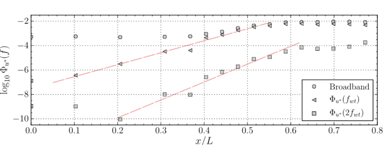
spectral densities, at f =fwt, triangles, and f = 2fwt, squares. . . 45
3.7 Streamwise evolution of the non-dimensional vorticity thicknessδω/δω0.
. . . 46
3.8 Power spectral density of the normalised velocity fluctuations u∗ =
u/ue, at three reference points: (a) - x/L = 0, y/δ0 − 3.4; (b)
-x/L = 0.58, y/δ0 = 0.45; (c) - x/L = 1.0, y/δ0 = −0.45. See figure
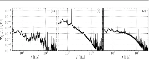
2.9 to locate the measurement points. . . 47
3.9 colour map of the power spectral density of the normalised velocity
fluctuations u∗ =
u/ue, at the frequency of the first mode fwt =
150Hz. The value is obtained by integration of the spectral density
in a band large 1 Hz around fwt.. . . 48
3.10 Power spectral density of the normalised pressure fluctuations p∗ =
2p/(ρu2e), for microphone m7, (a), microphone m8, (b) and
micro-phonem3, (c). Please refer to figure 2.9 for the exact positions of the
microphones. . . 49
3.11 Cross-correlation coefficient functions ρupj(τ). The velocity time
se-ries is measured at the reference point, x/L = 0.58, y/δ0 = 0.45.
Microphone m7, (a), microphone m8, (b) and microphone m3, (c).
Please refer to figure 2.9 for the exact positions of the microphones. . 50
3.12 colour map of the maximum absolute value of the cross-correlation
coefficient functions ρup7, across the entire shear layer.. . . 51
3.13 Squared coherence functions γup2 j. The velocity time series is
mea-sured at the reference point, x/L = 0.58, y/δ0 = 0.45. Microphone
m7, (a), microphonem8, (b) and microphone m3, (c). Please refer to
3.14 The colour maps show the spatial distribution of the reconstructed fluctuating velocity component in the shear layer in four selected time instants. The time delay between successive snapshots of the sequence
is 45∆t, where ∆t = 1/8000 s is the sampling interval. The grey
colour shading represents the modulus of the velocity fluctuation.
Eight iso-lines have been drawn for values of |uˆ′
/ue| equal to ±0.11,
±0.08, ±0.05, ±0.02; dashed contours indicate a negative value. . . . 54
3.15 Conceptual sketch explaining the moving wall effect.. . . 55
3.16 Comparison of the upstream x/L=−0.14, and downstream, x/L=
2.05, boundary layer mean velocity profiles, (a), and of the profiles of
the root-mean-square value of the velocity fluctuation, (b). . . 57
3.17 Snapshot sequence for CASE1 in the mid-span, sorted left to right,
top to bottom. . . 59
3.18 Mean value, top, and root-mean-square value, bottom, of the velocity
measured at x/L= 0.59, y/δ0 =−1.69, in the cavity region. . . 60
3.19 Spectra of the velocity fluctuations at z/b =−0.04 and z/b =−0.26
of the velocity fluctuation measured at x/L= 0.59, y/δ0 =−1.69, in
the cavity region. . . 61
3.20 Mean, top, and root-mean-square value, bottom of the velocity
fluctu-ation measured at x/L= 1.32, y/δ0 = 0.45, in the turbulent
bound-ary layer downstream of the cavity. . . 62
3.21 Profiles of u/ue, (a), and of u′
rms/ue, (b), for the upstream boundary
layer at x=−10 mm for CASE2. . . 63
3.22 Profiles of u/ue at several spatial locations along the shear layer.
One each three velocity profiles is shown for clarity. The downstream
cavity shoulder is also visible on the right. . . 64
3.23 Profiles of u′
rms/ue at several spatial locations along the shear layer.
One each three velocity profiles is shown for clarity. The downstream
cavity shoulder is also visible on the right. . . 65
3.24 Evolution of the shear layer vorticity thickness along the streamwise
direction. . . 67
3.25 Comparison of the upstream x/L=−0.14, and downstream, x/L=
2.05, boundary layer mean velocity profiles, (a), and of the profiles of
the root-mean-square value of the velocity fluctuation, (b). . . 67
3.26 Power spectral density of the normalised velocity fluctuations u∗ =
u/ue at three control points. . . 69
3.27 Example of velocity time history at control point B, located inside
the cavity at x/L= 0.58, y/δ0 =−0.68. . . 70
3.28 Pressure fluctuation spectra for three representative microphones.
The grey curve is the velocity spectrum at x/L= 0.58, y/δ0 =−1.1,
3.29 Profiles of max|ρupi(τ)| for microphones m7 located under the cusp,
m8 located in the impingement region, and m3, far downstream of
the cavity. . . 72
3.30 Cross-correlation coefficient function ρup(τ), where u is the velocity
signal inside the cavity region, at y/δ0 = −1.1, and p is that from
microphone m8, part (a), or microphone m7, part (b). . . 73
3.31 Squared coherence function γ2
up(f), where u is the velocity signal
in-side the cavity region, at x/L = 0.58, y/δ0 = −1.1, and p is the
pressure measured by microphone m8, part (a), or by microphone
m7, part (b).. . . 74
3.32 Snapshot sequence for CASE2, sorted left to right, top to bottom. Time interval between successive frames is 3/125 s. One of each three snapshots in shown, to complete almost a full revolution of the
vortex core. . . 75
3.33 Spanwise profiles in the cavity region at x/L = 0.58, y/δ0 = −1.36.
Mean velocity, (a), and root-mean-square value of the velocity
fluc-tuations, (b).. . . 77
3.34 Power spectral densities of the velocity fluctuations in the mid-span,
z/b = 0.0 lighter line, and at z/b = 0.43, darker line, where u′
rms/ue
is minimum. . . 77
4.1 Sketch of the cavity geometry showing the two regions where suction
was separately applied. . . 81
4.2 Effects of the suction rate on the mean velocity at a control point
downstream of the cavity, at x/L= 2.05, y/δ0 = 0.23. . . 82
4.3 Effects of the suction rate on the profiles of mean velocity and of the
root-mean-square value of the velocity fluctuations, at x/L = 2.05.
The upstream case and the no-control case are also reported. . . 83
4.4 Selected mean velocity profilesu(y)/uealong the shear layer.
Approx-imately one each four profiles is shown, for clarity. The downstream
edge of the cavity is also visible. Flow is from left to right. . . 84
4.5 Fraction of the height of the upstream boundary layer associated to
a given suction parameter S. . . 86
4.6 Sketch of the proposed boundary layer ingestion model. . . 86
4.7 Selected profiles ofu′
rms/uealong the shear layer. Approximately one
each four profiles is shown, for clarity. The downstream edge of the cavity is also visible. Flow is from left to right. The small vertical
segments indicate the value of u′
rms/ue = 0.1. The vertical dashed
line indicates the location where the profile is taken, and the value of
u′
rms/ue = 0 . . . 87
4.9 Effects of the suction rate on the mean velocity at a control point
inside the cavity region, at x/L= 0.58, y/δ0 =−2.27. . . 89
4.10 Snapshot of flow visualisation for CASE1 with suction, yq/δ0 ≈1.85 . 91
4.11 Power spectral density of the normalised velocity fluctuations u∗ =
u/ue at x/L = 0.58, and at a value y/δ0 corresponding to the peak
of the profiles of u′
rms/ue as of figure 4.8, for different values of the
suction parameter. Curve (a), S = 0; (b), S = 0.009; (c), S = 0.021; (d), S = 0.032; (e), S= 0.065; (f), S= 0.097. . . 92
4.12 Power spectral density distribution of the velocity fluctuations at
x/L= 0.58, across the entire shear layer, for S = 0.097. . . 93
4.13 Detail of the power spectral density of the normalised velocity
fluc-tuationsu∗ =
u/ue atx/L= 0.58 andy/δ0 =−2, for different values
of the suction parameter. Curve (a), S = 0; (b), S = 0.009; (c),
S = 0.021; (d), S = 0.032; (e), S = 0.065; (f), S = 0.097. . . 94
4.14 Distribution of the power spectral density of the velocity fluctuations
across the boundary layer at x/L= 2.05, for S = 0.037. . . 94
4.15 Effects of the suction rate on the spanwise profile of the mean velocity
at a control point in the cavity, at x/L= 0.58, y/δ0 =−2.27.. . . 96
4.16 Effects of the suction rate on the spanwise profile of the root-mean-square value of the velocity fluctuations at a control point in the
cavity, at x/L= 0.58, y/δ0 =−2.27. . . 97
4.17 Effects of the suction rate on the spectral distribution of the velocity
fluctuations at a control point in the cavity, at x/L = 0.58, y/δ0 =
−2.27. Figure (a), S = 0; (b), S = 0.009; (c), S = 0.032; (d),
S = 0.065; (e), S = 0.097. . . 98
4.18 Effects of the suction rate on the mean velocity at a control
down-stream of the cavity, at x/L= 2.05, y/δ0 = 0.045. . . 99
4.19 Effects of the suction rate on the profiles of u/ue and u′
rms/ue at the
downstream position x/L= 2.05. Profiles for the upstream reference
boundary layer are also reported. . . 100
4.20 Fraction of the height of the upstream boundary layer associated to
a given suction parameter S. . . 101
4.21 Effects of the suction rate on the profiles of u/ue and u′
rms/ue in the
shear layer region, at x/L= 0.58. . . 102
4.22 Selected mean velocity profiles along the shear layer for S = 0.054.
For each profile two vertical dashed lines indicate marks for u = 0
and u=ue. The first mark also indicates the x/Lposition where the
4.23 Selected profiles of u′
rms/ue along the shear layer for S = 0.054. For
each profile, the vertical dashed line indicates thex/Lposition where
the profile was measured and the valueu′
rms/ue = 0. The smaller red
segment indicates a mark for u′
rms/ue = 0.1, and its vertical position
follows the peak ofu′
rms/ue, whosey/δ0 position is indicated by a red
dot. . . 104
4.24 Spanwise profiles of the mean velocity at x/L= 0.58, y/δ0 = −0.45,
for several values of the suction parameter S, indicated in the figure.
The vertical red lines indicate the position of the ribs of the cavity
model, at which suction is interrupted for a width of 0.023b. . . 105
4.25 Spanwise profiles ofu′
rms/ue atx/L= 0.58, y/δ0 =−0.45, for several
values of the suction parameterS, (scale on the right), superimposed
to colour maps of the distributions of the energy of the velocity
fluc-tuations across the span. Figure (a): S = 0, (b): S = 0.008, (c):
S = 0.024, (d): S = 0.039, (e): S= 0.055. . . 106
4.26 Effects of the suction rate on the reduction of the momentum
thick-ness of the boundary layer at x/L= 2.05. The suction rate has been
rescaled using the parameter yq/δ0. . . 108
4.27 Comparison of the profiles ofu/ue, left, and ofu′
rms/ue, right, between
the suction regions A and B, for two conditions of suction, atx/L=
2.05. . . 109
4.28 Comparison of the profiles ofu/ue, left, and ofu′
rms/ue, right, between
the suction regions A and B, for two conditions of suction, atx/L=
0.58. . . 111
4.29 Snapshot sequence of the flow visualisation for CASE1 in the
mid-span, sorted left to right, top to bottom. S = 0.1. Time delay
between two subsequent snapshot is 3/400 s. . . 113
4.30 Comparison of the profiles ofu/ue, left, and ofu′
rms/ue, right, between
the suction regions A and B, for two conditions of suction, atx/L=
2.05. . . 114
4.31 Comparison of the profiles ofu/ue, left, and ofu′
rms/ue, right, between
the suction regions A and B, for two conditions of suction, atx/L=
0.58. . . 116
5.1 Color map of the mean jet velocityuj, as a function of the forcing
fre-quencyfj and the forcing voltage amplitudeAj, figure (a). Behaviour
of uj as a function offj, for three selected voltage amplitudes, figure
(b). . . 123
5.2 Color map of the mean velocity in x/L = 1.91, y/δ0 = 0.3, as a
5.3 Profiles of the mean velocity, (a), and of the root-mean-square value
of the velocity fluctuations (b), at x/L = 1.91, for different forcing
amplitudes, at fj = 75. The corresponding profiles for the upstream
laminar boundary layer are also shown for comparison. . . 126
5.4 Color map of the mean velocity inside the cavity, under the cusp at
x/L= 0, y =−2.27, as a function of synthetic jet control parameters. 127
5.5 Profiles of the normalised mean velocity, (a), and of the normalised
root-mean-square value of the velocity fluctuations (b), at x/L =
0.05, for different forcing amplitudes, at fj = 75 Hz. The no-control
condition is also shown for reference. . . 128
5.6 Mean velocity profiles across the shear layer in control conditions in
CASE1 with fj = 75 Hz and R= 1.29. . . 129
5.7 Profiles of the normalised root-mean-square value of the velocity fluc-tuationsu′
rms/ueacross the shear layer in control conditions in CASE1
with fj = 75 Hz and R= 1.29. . . 130
5.8 Color map of the mean velocity inside the cavity, under the cusp at
x/L= 0, y =−10 mm, as a function of synthetic jet control parameters.131
5.9 Profiles of the mean velocity, (a), and of the root-mean-square value
of the velocity fluctuations (b), at x/L = 0.58, for different forcing
amplitudes, at fj = 75 Hz. . . 132
5.10 Color map of the mean velocity downstream of the cell at x/L =
1.91, y/δ0 = 0.09, as a function of synthetic jet control parameters. . 133
5.11 Profiles of the mean velocity, (a), and of the root-mean-square value
of the velocity fluctuations (b), at x/L = 1.91, for different forcing
amplitudes at fj = 75 Hz. The upstream profiles are also reported
for comparison. . . 134
5.12 The colour maps show the power spectral densities of the velocity fluctuations across the boundary layer downstream of the cell at
x/L = 2.05, for three forcing conditions at fj = 75 Hz and in
no-control conditions. . . 135
5.13 Profiles of the mean velocity, (a), and of the root-mean-square value
of the velocity fluctuations (b), at x/L = 1.91, for different forcing
conditions atue = 5 m/s. The upstream profiles are also reported for
comparison. fj = 75 Hz. . . 137
5.14 Upstream/downstream boundary layer momentum thickness ratio as
a function of the jet velocity ratio, for all the investigated cases. . . . 138
5.15 Forcing amplitude-frequency spectrograms of the normalised velocity
fluctuations in x/L= 0.58, y/δ0 = 0, for several values of the forcing
6.1 Discrimination and re-sampling of the control signal, (a), and vector
representation of a candidate solution, (b). . . 145
6.2 Mean velocity percent increment at pointP as a function of the
forc-ing frequency of a pure sinusoidal control signal. The sine amplitude
is 1 Volt. . . 147
6.3 Objective function evolution history. . . 148
6.4 Optimized control signal. . . 149
6.5 Velocity time history measured at the slot exit for the optimized
sig-nal, (a), and for the sinusoidal signal at fj = 72 Hz, (b).. . . 150
6.6 Profile of the mean streamwise velocity u/ue, (a), and of the
root-mean-square value of the velocity fluctuationsu′
rms/ue, (b), at location
x/L= 2.05, downstream of the cavity. . . 151
7.1 Schematic of the closed-loop control system. . . 156
7.2 Example of controller’s poles and zeros on the complexz plane. Only
the positive imaginary half-plane is shown, since it is specular to the
negative half-plane, as the controller coefficients must be real. . . 159
7.3 Amplitude response, upper, and phase response, lower, of the
con-troller of figure 7.2 . . . 160
7.4 Sketch of the genome of a single individual controller. The controller
is defined by its zeros and by the gain. . . 162
7.5 Labview FPGA code implementing the closed-loop control logic . . . 163
7.6 Behaviour of an example controller in the initial generations. Time
history of the hot wire filtered voltage signal, (a), and time history of
the control signal, (b). Closed-loop control is switched on at t= 1 s. . 165
7.7 Behaviour of an example controller in “lock-in” conditions. Time
history of the hot wire filtered voltage signal, (a), and time history of
the control signal, (b). Closed-loop control is switched on at t= 1 s. . 166
7.8 Behaviour of an example controller after the optimisation process has come to the end. Time history of the hot wire filtered voltage signal,
(a), and time history of the control signal, (b). Closed-loop control is
List of Tables
3.1 Summary of the main parameters of the cases tested. The pedix 0
denotes quantities at the upstream reference station, atx/L=−0.14,
The main objective of this work is to investigate on the physics and on the control of the flow in a Trapped Vortex Cell, often referred to as TVC in the following. A TVC is a cavity with a particular geometry, which is optimised to trap a vortical structure. This configuration has recently gained interest has a device to control the flow past thick airfoils, but fundamental research is still required to make this technique effective.
Specifically, a first goal of this work is to investigate on the fundamental physics of this flow, by studying the basic elements and the dominant phenomena. In fact, this flow field is the result of the complex interaction of several flows, such as the upstream boundary layer, the shear layer detaching from the cavity leading edge, the vortex core, and the boundary layer developing downstream. A further issue of interest addressed in this work is that related to the role of unsteadiness of the cell flow, and in particular of the shear layer, whose self-sustained oscillations are a common feature of open-cavity flows.
The understanding of the driving physical mechanisms of the base flow is required to successfully proceed in developing a control strategy aiming at the control of the flow, because it is necessary to manipulate this flow in order to make the TVC an effective control device. Therefore, a second goal is to study and compare two different control techniques targeting the cavity flow. The first of the two is steady suction of the flow in the cell and has been already applied in past researches, but some additional insight into its effects on the base flow is required. The second proposed control technique is open-loop control with a synthetic jet actuator, a more efficient device whose unsteady action can couple to or drive the relevant mechanisms of the flow. Furthermore, open-loop control studies with a synthetic jet are propaedeutic for closed-loop control of the flow, briefly investigated in the last part of research.
This thesis is divided as follows. Chapter1presents a review of the literature re-garding aspects relevant to this research. Chapter2presents the experimental setup designed to address the above issues. Chapter 3 presents and discusses the results of the investigation on the basic uncontrolled flow, for two significant conditions. Chapter4and5discuss the result of control of the TVC flow using the two different
techniques. Chapter 4 discusses the effect of control by flow suction, while chapter
5 deals with the flow controlled by a synthetic jet actuator, and highlights the dif-ferences with the first control technique. In chapter 6 an optimisation procedure is carried out to search for the control signal which optimally controls the cavity flow. A preliminary discussion of closed-loop control studies is given in chapter7. Finally, conclusions of this work are detailed.
Review of the literature
1.1
Flow in a trapped vortex cell
A Trapped Vortex Cell is a particular cavity whose shape is designed as to trap a vortex. Such a configuration has been proposed,Chernyshenko[2009], as a device to control the flow past an airfoil, in order to enhance its aerodynamic performances. The basic idea of this control technique is to place a TVC on the upper surface of an airfoil, in a region close to the separation of the boundary layer, as depicted in figure
1.1. Then a suitable interaction of the incoming boundary layer with the cavity flow can result in a more energetic boundary layer downstream of the cell, with respect to the solid wall case, i.e. no cavity, which is less prone to separation, resulting in a lower drag and higher lift.
Figure 1.1. Schematic concept of an airfoil with TVC control.
The idea of trapping a vortex is not new as it was first mentioned by Ringleb
[1961]. Following this work, several applications of the trapped vortex concept for flow control have been studied. Adkins [1975] demonstrated experimentally that the pressure recovery in a short diffuser could be strongly enhanced by a stabilised trapped vortex. There are also two known examples of flight testing, namely the Kasper wing, (seeKasper [1974]) and the EKIP aircraft, (seeSavitsky et al.[1995]).
More recently, several investigations, theoretical, numerical and experimental, have been carried out in the framework of the EU project VortexCell2050, which had the objective of advancing the state-of-the-art of the technology of control by trapped vortex cells. Particular emphasis was given to study the characteristics of the vortex flow. In fact, one issue regarding this control technique concerns the inherent instability of the trapped vortex as a two dimensional flow. Theoretical work on trapped vortices, Chernyshenko et al. [2003], Zannetti [2006], Bunyakin
et al.[1998], has shown that a trapped vortex is usually unstable.
A three dimensional instability of the flow was also identified in both experimen-tal and numerical investigations. For exampleSavelsberg and Castro[2008] studied experimentally the flow inside a large aspect ratio cylindrical cell. In this case, the flow in the cavity, driven by the shear layer forming in the opening, showed a nearly solid body rotation, with low turbulence level in the vortex core. These authors noticed a significant distortion into an “S” shape of the mean velocity profile, which the authors attributed to three dimensional effects. In fact, they observed a span-wise modulation of the entire cells flow, which they suggested to be due to a natural three-dimensional instability. Further work by the same authors,Tutty et al. [2012], confirmed their hypothesis.
This spanwise modulation was also observed in a large eddy simulation performed
byHokpunna and Manhart[2007]. The authors argued that the three-dimensionality
of the flow is due to an inviscid instability of the vortex core, and also showed the appearance of a marked spanwise modulation of the Reynolds stresses along the cavity span. However, no specific indication of the effects of such three dimensional instability on the effectiveness of the TVC a a control technique was given by the above authors.
Nevertheless, the problem of stability of the trapped vortex flow directly leads to the problem of its control. A first solution is passive control of the flow which can be realised by careful design of the cavity geometry. For example,Chernyshenko et al.
[2008] set up an evolutionary algorithm to search in the space of cavity geometries for that which reduces internal secondary separation of the cell’s flow, which is an undesirable feature of this flow. Active control of the cavity flow has been also investigated. De Gregorio and Fraioli [2008] have investigated experimentally, by means of PIV measurements, the effectiveness of a cavity located on an airfoil. The upstream interior part of the cavity was porous, in order to allow suction of the flow. Unfortunately, their setup did not allow to measure lift and drag of the controlled airfoil, since the airfoil was embedded on the bottom surface of the wind tunnel. Nevertheless, the effectiveness of the control was assessed by considering the size of the region of separated flow downstream of the cavity. The authors observed that, in passive conditions, i.e. no suction, the sole presence of the cavity yielded performances poorer than that of a clean airfoil, with a large separation region starting from the cavity cusp. By gradually increasing the suction, they
0.0 0.1 0.2 0.3 0.4 0.5 0.6 0.7 0.8 0.9 1.0 x/c −0.2 −0.1 0.0 0.1 0.2 0.3 y /c a bc d e
Static pressure taps Kulite sensors
Figure 1.2. Drawing of the airfoil with the trapped vortex cell
tested byLasagna et al. [2011]
observed the formation of a coherent vortex in the cavity, accompanied by partial flow reattachment and by a decrease of the separation region downstream of the cell itself.
A further investigation of the TVC technique is the wind tunnel testing of a thick airfoil equipped with a TVC control device, performed byLasagna et al.[2011]. This work is briefly discussed here, since it is the most relevant work for this project.
The airfoil chosen was a thick NACA0024 profile. Several configuration were tested and compared: the baseline NACA0024 profile, (B), the same profile but with a classical boundary layer suction system, (BS), and a NACA0024 profile equipped with a TVC, as in figure, 1.2. The latter configuration featured a porous cavity surface, in order to apply suction in the cavity region, similarly to what performed
byDe Gregorio and Fraioli[2008], resulting in the configurations TVC, no suction,
and TVCS, with suction. Aerodynamic coefficients were measured by integration of the static pressure distribution, for the lift, and by momentum balance, for the drag. Tests were mainly performed at a chord-based Reynolds number of 106.
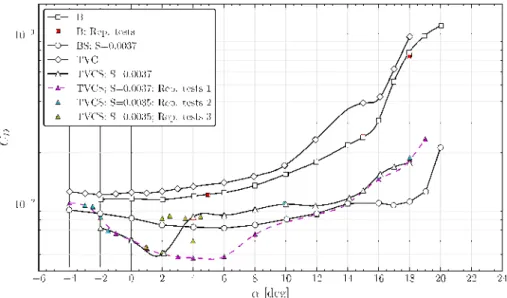
The lift coefficient results of the four configurations tested are reported in figure
1.3. The results indicates that the TVC configuration with no suction, i.e. passive control, yields virtually no improvements, since the lift coefficient is essentially the same of the B configuration, if not worse. However, when suction is applied to the trapped vortex cell the lift increases, by a small amount at small-to-medium incidences, and by a larger, but not exceptional, amount at high incidences. In any case, in terms of lift, the performance of the TVCS configuration were never
superior to that of the classical boundary layer suction system, BS, neither at low nor at high incidences. The explanation provided by Lasagna et al. [2011] for the larger lift observed at high incidences for the TVCS, and BS, configurations is the delay of flow separation on the upper surface of the airfoil, mainly due to the suction applied in this region, in spite of the way this suction was applied, i.e. at the wall of the clean airfoil, or in the cavity region.
Figure 1.3. Lift coefficient curves for the four configurations tested
inLasagna et al. [2011].
Much more revealing were the drag coefficients curves, reported in figure 1.4. The results indicated that the TVC is not effective as a passive control device, since
Figure 1.4. Drag coefficient curves for the four configurations tested
inLasagna et al. [2011].
the drag of the TVC configuration, open diamonds, always resulted in a drag larger than that of the baseline configuration, open squares, from small to large incidences. In stark contrast, the drag curve of the TVCS configuration was significantly below that of the baseline configuration, for all the incidences. However, complex
behaviour was observed for this configuration. In fact, results of several tests per-formed on this configuration, in slightly different experimental conditions, gave rise to a bifurcative behaviour, with two branches separating atα = 2◦, merging again at
aroundα≈14◦. These two branches were called low-drag and high-drag branches,
for obvious reasons. A similar behaviour was observed atα =−2◦, where the drag
curve of the TVCS configuration showed a sudden decrease inCD, from a high-drag
to a low-drag mode. The observed drag reduction with respect to the baseline case is significant and it was larger than 50% at α = 6◦, although a strong amount
of suction was required to achieve this result, with a strongly unfavourable energy balance.
However, the most important results of this research was that, despite this com-plex behaviour, in a narrow range of incidence, mostly at small angles of attack, −2◦
< α < 10◦, the TVCS system resulted in a drag coefficient significantly lower
than that of the BS configuration, for the same amount of suction.
Spectral analyses of the pressure fluctuation signals, measured by Kulite pressure transducers mounted in the region of the cell, see figure 1.2, indicated that the two drag modes were characterised by two very different flow regimes. It was postulated that in the low-drag mode the cavity was filled with a very stable and coherent vortical structure, with the shear layer displaying a characteristic Kelvin-Helmoltz instability, clearly evidenced in the power spectral density plots as a sequence of sharp peaks, at frequencies well matching results on rectangular cavity flows, i.e. at a Strouhal number based on the cavity length of the order of the unity. By contrast, in the high-drag mode, the spectra of the pressure signals displayed a very large energy peak at a very low frequency, at a Strouhal number about 0.065. This peak was associated to the presence of a “wake mode”, that is a large scale, low frequency flow regime reported in the literature of rectangular cavity flows. These results clearly pointed out the relevance of unsteady phenomena for this control technique of which they strongly influence the effectiveness.
To explain such a large reduction in drag and the better performances with respect to the BS configuration, the “moving-wall” effect introduced byDonelli et al.
[2009] was proposed. This mechanism suggests that the “moving surface” generated by the vortex flow, replacing the solid wall of the baseline airfoil, results in a wall flow downstream of the cell more energetic and thus less prone to separation, than the baseline case. Lasagna et al. [2011] added that, for small incidences, where the flow is fully attached and pressure drag is limited, the more energetic boundary layer would be characterized by a lower momentum thickness up to the trailing edge, resulting in a narrower wake, that is in a lower drag. It must be noted that in the experiments ofLasagna et al.[2011], this mechanism has only been postulated and no direct evidence was actually observed, due to limited measurements. Furthermore, very few results are available in the literature that provide specific evidence of this mechanism.
Control of the flow over a thick airfoil with a cavity was also investigated by
Ols-man and Colonius[2011]. These authors investigated by direct numerical simulation
and by flow visualisations in a water tunnel the passive control on a low-Reynolds-number flow, atRec = 2·104, wherecis the airfoil’s chord. These authors evidenced
a very complex interaction between the structures generated by the cavity shear layer, subject to a Kelvin-Helmoltz instability, and the separated flow downstream of the cavity, which eventually resulted in an increase of the lift-to-drag ratio of the airfoil. The control mechanism found by the authors is fundamentally different to that proposed by Donelli et al. [2009], even though its effects may become less pronounced at higher Reynolds number conditions.
1.2
Flows in canonical rectangular cavities
We present here a short review of the literature regarding the main issues of the physics and the control of flow in rectangular cavities. It is argued that despite the different geometry, they share some many common issues and phenomena with trapped vortex cells. Furthermore, such configurations have been extensively studied in the past decades since they have important practical applications in aerospace and industry, but also because they are an important and challenging canonical flow to design control strategies,Rowley and Williams [2006]. Because of this large body of research, it may be easier to interpret the physics of the flow in a trapped vortex cell, as well as designing effective control strategies. Furthermore, few research studies have focused on using cavities as control devices for fluid flows, and, thus, this work adds insight into this topic.
1.2.1
Unsteady phenomena
The most significant dynamical feature of cavity flows, and studied in depth, is that they often develop strong oscillations of velocity field, strongly coupled with intense fluctuations of the acoustic field. The accepted mechanism explaining such phenomenon is represented in figure 1.5 and is known at least from the pioneering work of Rossiter [1964]. The upstream boundary layer, with a given thickness δ and momentum thickness θ, detaches at the leading edge of the cavity and evolves downstream spanning the entire length L of the cavity. The shear layer eventu-ally impinges on the downstream edge of the cavity where strong acoustic waves are scattered and travel upstream. When an acoustic wave arrives at the cavity leading edge, it develops into a flow perturbation depending on the receptivity of the separating boundary layer layer. Such initial perturbations are amplified by the instability of the shear layer, strongly determined by its mean velocity profile, and eventually saturate developing coherent spanwise rollers of vorticity, which, at the
Figure 1.5. Schematic showing the mechanism determining self-sustained oscillation of the shear layer in a rectangular cavity flow. Taken from Cattafesta et al.[2008].
impingement produce strong acoustic wake, resulting in a feedback process. This mechanism results in very well defined spectral peaks at distinct frequencies and produce strong resonant oscillation, also known as cavity or Rossiter tones.
For compressible flows, the frequencies of the resonant tones can be predicted with good accuracy with Rossiter equation:
fn=
ue
L
n−α
M + 1/k (1.1)
where fn is the frequency of the n-th mode, α is a parameter which takes into
account the phase lag between the impingement of a coherent structure and the production of an acoustic wave, k defines the ratio of the phase velocity of the convective disturbances in the shear layer to the external velocity, while M is the freestream Mach number.
The intense acoustic field resulting from this mechanism produce strong unsteady loads which may lead to structural damages and, therefore, the study of its physics has a profound impact in many applications, such as landing gear and weapon bays,
Bruggeman et al. [1991], sunroofs and windows in automobiles, Mongeau et al.
[1997], as well as in many other industrial applications.
A further unsteady phenomenon which may characterise a cavity flow is the wake mode oscillation, observed experimentally by Gharib and Roshko [1987] and in numerical simulations byRowley et al.[2001] andSuponistsky et al. [2005]. This mechanism is dominated by a low frequency large scale vortex shedding, similar to the shedding of vortices in the wake of bluff bodies. Such a regime is associated to an increase of the cavity drag, with large amplitude fluctuations at a Strouhal
number of the order of 0.07. As pointed out byRowley et al.[2001], this mechanism is not due to acoustics, but it is the result of an absolute global instability of the cavity flow.
1.2.2
Three dimensional properties
Although the geometry of a rectangular cavity is simple, the flow topology is highly complex and, as several workers have reported, it is essentially three-dimensional.
Maull and East[1963] first documented the strong three dimensional nature of this
flow with oil visualisations showing the occurrence of a cell-like structure of the flow. They reported that this flow organisation was found only when the cavity span was set to certain values: the steadiest and most regular conditions were found when the cavity span was an integral number of cell spans. They also noted a strong influence of this particular flow topology on the spanwise pressure distribution in the cavity. In fact, a periodic modulation of the pressure was present, with a period roughly equal to twice the cavity length.
The occurrence of such spanwise modulation in the flow characteristics at high Reynolds numbers was also confirmed in recent LES simulations performed by
Larchevêque et al. [2007]. They have also found these modulations to be caused
by the presence of a cell-like organisation of the flow. They report of a bifurcative behaviour of the flow, with two possible asymmetrical flow solutions, being mirror images of each other and which could be selected by imposing a different asymmetric in-flow condition. They also report of a transient, less stable symmetrical configu-ration, which would occasionally break-down into one of the two non symmetrical configurations. Three-dimensional characteristics have been also found if the shear layer region, as reported by Rockwell and Knisely[1980]. Direct observation of the flow revealed a coupling between the roll-up of the primary spanwise vortices in the mixing layer with the growth of secondary streamwise vortices, which led to a severe distortion of the primary vortices.
The above studies found three dimensional characteristics which have a length scale of the same size of the cavity dimension. However, other studies have demon-strated the presence of small scale coherent three dimensional structures such as Taylor-Gortler like vortices, as found by Faure et al. [2009]. These authors have demonstrated that the occurrence of such structures is strongly tied to a centrifu-gal instability due to the curvature of the flow in the recirculation region, which trigger the formation of such structures. Similar conclusions were drawn byMigeon
[2002], which examined the details of the flow start up in a square lid driven cavity experiment, observing the presence of such vortices.
1.2.3
Recirculating flow
A further important element is the recirculating flow inside the cavity. The structure of this flow is strongly dependent on the geometrical characteristics of the cavity, and mainly by the ratio L/D, where L is the cavity length and D is the cavity depth, see for example Faure et al. [2006]. The typical structure is composed of a main recirculating flow. If the ratio L/D is high enough, the interaction of the main vortex with the fluid upstream of it may result in the formation of a secondary counter-rotating vortex. Typically, corner vortices may also develop.
It has been shown that there is a clear interaction between the recirculating cavity flow and the shear layer evolution. In fact, Lin and Rockwell [2001] suggest that the large-scale flow structures in the recirculating zone may affect the disturbance growth in the shear layer and consequently the oscillating nature of the overall flow.
Kuo and Huang[2001] studied the effects on the oscillations of the cavity shear
layer by introducing flow path modifier and by modifying the slope of the bottom surface of the cavity itself. The authors observed, by both flow visualisations and LDV measurements, that the upstream part of the recirculating flow have an im-portant effect on the instability characteristics of the shear layer.
Design of the experiment
This chapter presents the experimental setup designed and realised for the investiga-tion. It discusses the basic rationale behind the chosen configuration and describes all the components. The hardware required for the two control techniques is also pre-sented, leaving a thorough discussion to their respective chapters. Instrumentation, other hardware and measurement techniques are also documented.
2.1
Design rationale
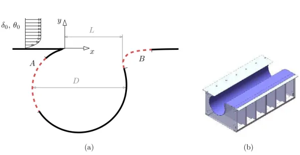
The configuration chosen for the experimental investigation is a TVC embedded onto the bottom flat surface of the wind tunnel test section, as sketched in figure
2.1.
wind tunnel bottom wall
Figure 2.1. Sketch of the simplified configuration chosen for the experi-mental investigation.
This configuration differs from that of the TVC equipped airfoil mainly by the fact that there is no external pressure gradient imposed on the cell. The chosen configuration is simpler since it purposely eliminates some of the phenomena present on the airfoil, such as flow separation or wake dynamics, and the possible couplings between the cavity flow, the wake and the separated region. It is argued that separation of these effect, tough a strong simplifying assumption, is paramount to ease the effort of understanding basic mechanisms.
This simplified configuration is chosen since the main objective of the research project is focused towards the understanding of the physics of the TVC flow itself. In this regards, the aerodynamic performance of a TVC controlled airfoil were not in the scope of this particular project, but connections between the two configurations will be often made. In fact, it is argued that the performances of the cell in controlling the flow over the complete airfoil are strongly connected to how the cell itself modifies the boundary layer flowing past it, for example by increasing the mean velocities in the near-wall flow downstream of it. Such effects can be easily studied on the simplified configuration and may shed some light over the control of the flow on the complete airfoil.
Nevertheless, the extent by which the full airfoil configuration differs from the chosen simplified configuration and how the basic mechanisms discussed in this work are affected must certainly be the object of future research.
2.2
The wind tunnel
The open-circuit blower wind tunnel "Fucsia", shown in figure 2.2, was chosen for the experiments. It is a small facility, adapt for fundamental research studies. The test section of the wind tunnel is long more then 4 meters and, in the region chosen for the investigation, it has a width and a height of 750 and 550 mm, respectively. The maximum speed is of the order of 14 m/s.
Figure 2.2. Front and rear views of the “Fucsia” wind tunnel used for the investigation.
2.2.1
Modifications to the wind tunnel test section
A large amount of design and work has been dedicated to modify the test section region. A first task has been to raise the bottom wall of the test section by about 200
mm, in order mainly to leave space for the cavity model and for instrumentation. This task was accomplished by designing a support system, adaptable in height, covered with flat panels spanning the full width and length of the test section area. The reduction of the test section area also resulted in a increase of the maximum velocity. Furthermore, a ramp was positioned in the first region of the test section to smoothly recover the difference in height between the two sections. This region of the test section has been checked by smoke flow visualisations to not produce inconvenient separated regions, which would introduce spurious fluctuations into the boundary layer flow. The left picture in figure 2.3 show a detail of the convergent ramp and the adjustable support system. The picture on the right shows instead the flat panels recreating the bottom wall of the test section.
Figure 2.3. Pictures of the convergent ramp, supports and flat panels.
A second important task has been to modify the test section in order to allow both optical and manual access to the investigation area. To this end, the two lateral walls of the test section have been replaced by transparent Plexiglas panels. One of them was also designed to be easily removable to provide operation access to the investigation area.
Particular attention has been paid to the design of the top wall. The requirements for this element were: it should provide full optical access from above, (mainly to a laser sheet for flow visualisations) and it should give a mean to hold hot wire probes and to move them in the three directions. In order to satisfy these requirements the top wall was manufactured with a large Plexiglas panel, with a long longitudinal slot in its centerline to allow the insertion and the motion of a probe holder into the flow or of a laser sheet. The panel was supported on the two longitudinal ends by two spanwise rail guides, providing an adjustable displacement of the panel slot along the spanwise direction. The left picture in figure 2.4 shows a CAD model of the top panel.
Figure 2.4. On the left: CAD model of the wind tunnel test section, with details of the top panel supported by two spanwise rails. On the right: picture of the top panel, showing also the probe traverse system.
2.3
The probe traverse system
One of the requirements of the experimental setup was to achieve a full automati-sation of the probe motion, such as to minimise run times. To this end, a two-axes traverse system equipped with stepper motors was positioned above the top panel, outside of the test section, on two longitudinal rails. The right picture in figure
2.4 shows a picture of the traverse system in place. This configuration allowed fine control of the streamwise and vertical position of the probe, while control in the spanwise was achieved by manual displacement of the entire top panel along the two spanwise rails. Furthermore, fast but uncontrolled motion along the streamwise direction was obtained by sliding the entire positioning system along the two longi-tudinal rails. The stepper motors were driven by their power supply units, usually controlled by a Labview system. This allowed, for example, to semi-automatise the entire motion-acquisition process, saving significant time.
2.4
The boundary layer suction system
It is known that the flow regime in a cavity is markedly affected by the properties of the upstream boundary layer, and mainly by the ratio of the cavity length to momentum thickness L/θ, see e.g. Rockwell and Knisely [1980]. For this reason, a boundary layer suction system was designed to be located about 400 mm upstream of the cavity leading edge, in order to control the characteristics of the boundary layer detaching at the cavity cusp.
entire width of the test section, which replaces the corresponding region of the test section bottom wall. The plate covers a drawer embedded in the bottom wall and connected to a suction system, composed by a commercial blower for air condition-ing. Inside the drawer, dividing vanes ensure a good uniformity of the boundary layer properties across the span. This was checked by preliminary boundary layer measurements at the cavity leading edge. The flow rate of the blower was measured by measuring the difference between the pressure in the suction ducts and the am-bient pressure, which was previously correlated against the flow rate by measuring the exit velocity on a fine grid over the exit section of the blower.
The suction system was tested at different wind tunnel speeds and suction rates and for each test condition a boundary layer profile was measured, in the mid-span section and at 10 mm upstream of the cavity cusp. As an example, at a flow speed equal to 6 m/s, at which a significant part of the tests has been conducted, the boundary layer momentum thickness could be varied within 0.6 and 3 mm.
Preliminary investigations were dedicated to asses the uniformity of the incom-ing flow and to tune the experimental apparatus, in particular the boundary layer suction system and small details in the junctions between the elements of the bottom surface.
2.5
The cavity model
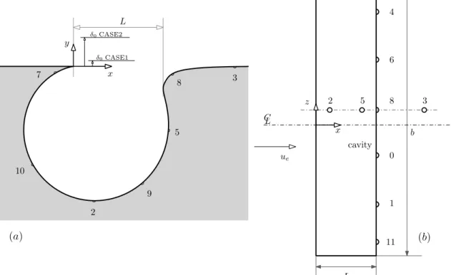
The geometry chosen for the experiments, shown in figure 2.5-(a), is identical to that of the numerical simulation of Hokpunna and Manhart [2007]. In the figure, the reference system adopted is also shown, together with the symbols of the main parameters of this geometry.
The cavity opening lengthLis the projection along thexaxis of the cavity open-ing,D is a characteristic diameter of the cell, taken as the largest distance between the upstream and downstream faces of the cell. δ0 and θ0 are the 99% boundary layer thickness and momentum thickness of the reference upstream boundary layer, measured atx/L=−0.14, i.e. x=−10 mm, in the mid-span section. The lettersA and B denotes the two regions were suction was applied to control the cavity flow, as will be discussed later.
The choice of the cavity sizes, mainly the opening length L and its span b, not indicated in the figure, was driven by several requirements and constraints. One of the most important requirement was the achievable range of values for fundamental parameters of the flow, such as the cavity Reynolds numberReLor the ratio opening
length to momentum thickness L/θ. The manufacturing process, availability of materials, the size of various probes were also important aspects of the design. In the final configuration, the cavity had a nominal opening length equal to L = 68 mm and a span b of 420 mm, so that the aspect ratio was about 6.6. The internal
L x y D δ0, θ0 A B (a) (b)
Figure 2.5. Sketch of the cavity geometry and of the reference system, (a), and CAD drawing of the cavity model, (b).
diameter of the cavityDwas equal to 114 mm. The cavity spanned 56% of the test section width, leaving a free space of about 160 mm between the cavity ends and the vertical test section walls. This prevented interactions between the corner flows developing at the angles of the test section with the cavity flow.
The cavity model was built as a ribbed structure with Plexiglas material, as shown in figure2.5-(b), with transverse rods to keep the model in place. This solid structure was then covered with a transparent 0.5 mm poly-carbonate film, which further improved the stiffness of the model. The thickness of the film was chosen to be as large as the manufacturing process allowed, in order to prevent fluid-structure coupling induced by the fluid oscillations that were expected. Appropriate care was taken to ensure that the poly-carbonate film remained attached to the ribs, to maintain the geometry.
2.6
The cavity suction system
One of the active control techniques which have been investigated is that of suction of the cavity flow. As represented in figure2.5-(a) two regions were chosen to apply suction, and the motivations are briefly discussed here. The first, denoted by letter A, was motivated by the idea of manipulating the structure of the flow inside the cell. Furthermore, this same region was investigated by other authors, e.g. Lasagna
et al. [2011] and De Gregorio and Fraioli [2008]. On the other hand, suction in the
second region, denoted by B, was chosen with the idea of manipulating the flow near the impingement region, which, in no control conditions, is a region of strong
unsteadiness. An in depth discussion of the motivations behind these choices is given in chapter 4, devoted to the discussion of the control with suction.
The solution adopted to perform suction of the flow has been to make the poly-carbonate film porous, by drilling many small holes in the chosen suction area. Holes of 1.5 mm where drilled on a square pattern with edge equal to 5 mm, thus making an equivalent porosity equal to 12.5%. Figure2.6shows a picture of the porous wall on the downstream edge of the cavity, in region B.
Figure 2.6. Detail of the porous surface on the downstream cavity edge, in region B.
Please note that the two regions have been manufactured on the same poly-carbonate sheet, but tests were conducted separately, by covering one of the two regions with a thin, less than 0.1 mm, adhesive film.
The entire Plexiglas cavity model was then embedded into a watertight drawer, connected to a suction pump located outside the wind tunnel. A flow meter and a regulating valve, connected into the pneumatic line, provided means to measure and vary the suction rate, respectively.
2.7
The synthetic jet system
The second control technique investigated is based on a synthetic jet actuator. A drawing of the actuator system configuration is shown in figure 2.7.
The injection location is located on the downstream side of the cavity and it is directed tangentially into the cavity. The idea behind this particular positioning is to inject momentum into the cavity, such as to favour the formation of an intense
x y
δ0, θ0
loudspeaker
synthetic jet box synthetic jet slot
Figure 2.7. Sketch of the side view of the cavity with the synthetic jet actuator.
vortical structure. The injection slot was actually divided along the span into six 60 mm slots separated by 10 mm due to the presence of the cavity ribs. The six slots were fed by watertight plenum chambers connected in couples to the actuators. These consists of three 4 Ω 150 Watt loudspeakers, driven by a Coraline power amplifier, each driving two slots.
Control of the loudspeaker input signal was performed via a NI9263 Analog Output module, controlled by an appropriate Labview program, implementing a signal generator. Such a flexible arrangement provided a significant step in task automatisation and provided a strict control on the input signal waveform.
2.8
Measurements techniques
To investigate the cavity flow two measurement techniques were used, namely hot-wire anemometry for the velocity in the flow field and condenser microphones to measure pressure fluctuations at the wall.
Hot-wire anemometry Extensive velocity measurements were performed us-ing constant temperature hot wire anemometry. An A.A. LabSystems AN1003 anemometer with a built-in signal conditioning unit was used to measure the veloc-ity component normal to sensor. A single-wire probe, (length 0.9 mm and diameter 5µmm). The probe was frequently calibrated in situ, in the middle of the vein and at a sufficient distance upstream of the cavity to render negligible its influence.
The probe holder was tilted by about 40 degrees with respect to the freestream direction, as shown in figure 2.8, in order to minimise its protrusion into the shear layer and into the cavity flow.
Figure 2.8. Detail of the hot wire probe holder. Flow is from left to right.
Pressure fluctuation measurements Pressure fluctuation measurements were performed using high-sensitivity electret condenser microphones, of a similar type as those used by other authors, e.g. Zhang and Naguib [2011], Garcia-Sagrado and
Hynes [2011]. Twelve microphones were positioned allover the cavity model, and
their location is shown in figure 2.9. Figure (a) shows a side view of the cavity
ue b cavity 11 1 0 8 6 4 L 8 3 5 9 2 10 7 L x y 2 5 3 CL (a) (b) z x CASE2 δ0 CASE1 δ0
Figure 2.9. Sketch of the side view of the cavity model at the span of the central row of microphones, (a); top view (b).
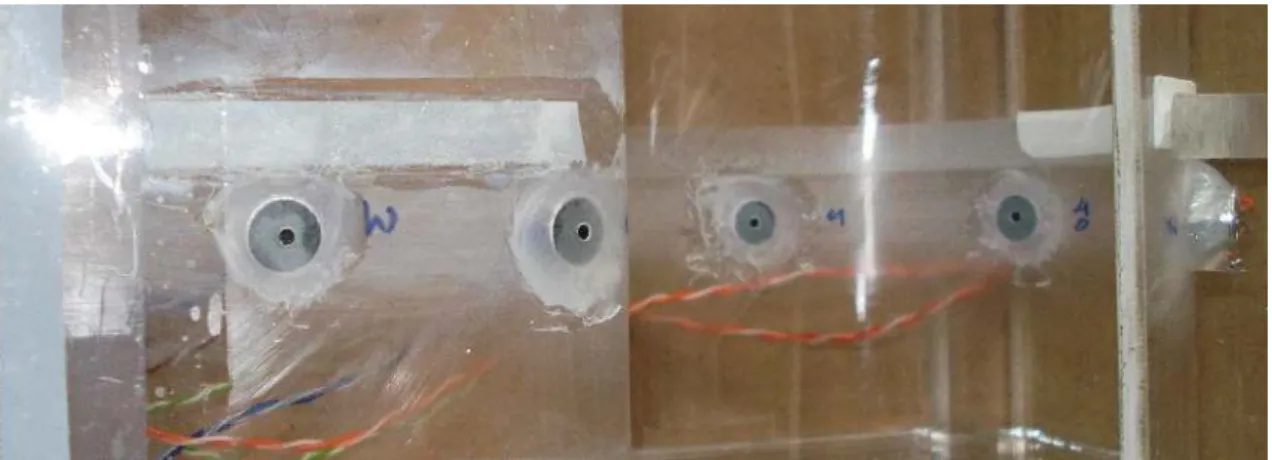
model, in a section about 15 mm away from the centerline of the cavity span, due to the presence of a rib in the mid-span section. The figure also show the relative thickness of the boundary layer for the two conditions extensively investigated in this work, CASE1 and CASE2, discussed later. This figure serves as a reference for the discussion of the results presented later, since the measurement location will be often given in non dimensional units,x/L and y/δ0. Figure (b) shows a top view of the cavity model, showing the position of the microphones located along the span, on the downstream edge of the cavity. These microphones were spaced along the span by 65 mm, and their signals were used mainly to assess the 2D properties of the shear layer flow.
The microphones, with a diameter and height of 9.7 and 6 mm, respectively, were powered by a dedicated power supply unit through custom-made RC circuits. These microphones, which only measure the fluctuating component, were positioned under the poly-carbonate film of the cavity, and aligned with a 2 mm hole. The large diameter of the hole was chosen as a compromise between the need to maximise the signal to noise ratio and minimisation of spatial filtering effects. Figure 2.10 shows a picture taken from the top of the central row of microphones. The microphone holes, the silicone mountings and the wires are also visible.
Figure 2.10. Top view of the central row of condenser microphones.
Seven microphones were located in a section of the cavity 15 mm away from the mid-span, as shown in figure2.9. Five other microphones were located transversely along the downstream shoulder of the cavity in the same position of microphonem8 with a spacing of 60 mm.
The dynamic properties of the microphones were estimated by an ad-hoc calibra-tion similar to that performed byZhang and Naguib [2011] andGarcia-Sagrado and
Hynes [2011]. The objective of the calibration was to find the microphone transfer
functionH(f). These dynamic properties are summarised in terms of gain in mV/Pa and phase delay, as a function of the frequency. The calibration setup consisted in a
flat plate located at a distance of 50 cm in front of a high power loudspeaker, which produced a fluctuating pressure field on the plate. The electret microphones were positioned on this plate with the same arrangement of the measurements described above. A reference high-precision microphone was flush-mounted in the centre of the plate. This was a high quality 1/4" Brüel&Kjær (type 4939) condenser microphone. This microphone has pre-amplification, flat frequency response in the range 10-10000 Hz and selectable gain by means of a dedicated power-supply/signal conditioning unit.
The microphones calibration was performed according to system identification procedures, described in detail byLjung[1998]. A zero-mean Gaussian noise, pass-band filtered between 2 and 2500 Hz, was fed to the loudspeaker through an ampli-fier. Because the loudspeaker signal values was sampled from a Gaussian distribu-tion, large values exceeding the input capability of the loudspeaker could occur. For this reason the signal was clipped between ±eth, a chosen threshold voltage.
How-ever, since clipping the signal in the time domain affects the signal spectrum in the frequency domain, the clipping and band-pass filtering were repeatedly applied to the signal, until it reached satisfactory time and frequency domain characteristics.
Simultaneous measurements from the electret and the B&K microphone were sampled at a frequency of 10 kHz and for 120 s. The length of the time histories was such as to provide satisfactory convergence of the spectral characteristics of the signals. Transfer function estimates, evaluated according to Bendat and Piersol
[1986], were then obtained as:
H(f) = ΦBm(f) ΦBB(f)
(2.1) where ΦBm(f) is the cross-spectral density between the voltage signal of the electret
microphone and the pressure signal of the B&K microphone, while ΦBB(f) is the
power-spectral density of the B&K microphone signal. All the spectral densities were obtained via the Welch algorithm, to improve the quality of the spectral density estimate.
Amplitude and phase response plots were analysed in detail for each microphone under test. As expected, the microphones significantly attenuated low-range fre-quency components below 10 Hz. The gain of each microphone was found to be suf-ficiently constant in the band 20-1000 Hz, in which most of the shear layer dynamics were expected, and was practically constant in successive calibration experiments. The phase shift introduced by the microphone was found to be negligible, of the order of 50 µs in the frequency range of interest. For this reason, it was not taken into account in the subsequent analyses. Furthermore, resonance effects due to the arrangement were not observed. Finally, in order to test the linearity properties of the microphones, different calibration experiments with different amplitude of the