Vol. 15, No. 1 (Full Issue)

Volume 15 | Issue 1 Article 51

5-1-2016

Vol. 15, No. 1 (Full Issue)

JMASM Editors

Follow this and additional works at:http://digitalcommons.wayne.edu/jmasm

This Full Issue is brought to you for free and open access by the Open Access Journals at DigitalCommons@WayneState. It has been accepted for

Recommended Citation

Editors, JMASM (2016) "Vol. 15, No. 1 (Full Issue),"Journal of Modern Applied Statistical Methods: Vol. 15 : Iss. 1 , Article 51. DOI: 10.22237/jmasm/1462078200

ii

Journal of

Modern Applied

Statistical Methods

Department of Psychology University of Manitoba

Jack Sawilowsky EDITOR

Reason Statistical Consulting

Alan Klockars

ASSISTANT EDITOR EMERITUS

Educational Psychology University of Washington Bruno D. Zumbo

ASSOCIATE EDITOR

Measurement, Evaluation, & Research Methodology University of British Columbia

Vance W. Berger ASSISTANT EDITOR

Biometry Research Group National Cancer Institute

Todd C. Headrick ASSISTANT EDITOR

Educational Psychology & Special Education So. Illinois University−

Carbondale

Clayton Hayes

EDITORIAL ASSISTANCE

Joshua Neds-Fox

EDITORIAL ASSISTANCE

Heather Marie Perrone

EDITORIAL ASSISTANCE

JMASM (ISSN 1538−9472, http://digitalcommons.wayne.edu/jmasm) is an independent, open access electronic journal, published biannually in May and November by JMASM Inc. (PO Box 48023, Oak Park, MI, 48237) in collaboration with the Wayne State University Library System. JMASM seeks to publish (1) new statistical tests or procedures, or the comparison of existing statistical tests or procedures, using computer-intensive Monte Carlo, bootstrap, jackknife, or resampling methods, (2) the study of nonparametric, robust, permutation, exact, and approximate randomization methods, and (3) applications of computer programming, preferably in Fortran (all other programming environments are welcome), related to statistical algorithms, pseudo- random number generators, simulation techniques, and self-contained executable code to carry out new or interesting statistical methods.

Journal correspondence (other than manuscript submissions) and requests for advertising may be forwarded to

Journal of Modern Applied Statistical Methods

Vol. 15, No. 1



May 2016



Table of Contents



Invited Articles

2 – 11 J. R. LEVIN The Composite Hypothesis Contrast Procedure:

R. C. SERLIN A Novel Sequential Multiple-Comparison

Approach

12 – 31 R. R. WILCOX ANCOVA: A Global Test Based On

A Robust Measure of Location or Quantiles When There Is Curvature

32 – 61 H. J. KESELMAN Generalized Linear Model Analyses

A. R. OTHMAN For Treatment Group Equality

R. R. WILCOX When Data Are Non-Normal

62 – 77 R. R. WILCOX Comparisons of Two Quantile Regression

Smoothers

Regular Articles

78 – 99 J. FEYS New Nonparametric Rank Tests for Interactions

In Factorial Designs with Repeated Measures

100 – 122 G. L. BAIRD Does One Size Fit All? A Case for Context-

L. L. HARLOW Driven Null Hypothesis Statistical Testing

123 – 140 C. H. HOLLAND A Two and More Independent Factor Form of

T. HOLLAND the Wilcoxon-Mann-Witney Test, Extendable

iv

141 – 159 D. T. NGUYEN Parametric Tests for Two Population Means

E. S. KIM under Normal and Non-Normal Distributions

P. RODRIGUEZ DE GIL

A. KELLERMAN

Y. -H. CHEN

J. D. KROMREY

A. BELLARA

160 – 192 M. DESAI Multiple Imputation When Rate of Change

A. A. MITANI is the Outcome of Interest

S. W. BRYSON T. ROBINSON

193 – 205 R. ARUNACHALAM Construction of Pair wise Balanced Design

M. SIVASUBRAMANIAN

D. K. GHOSH

206 – 238 B. M. GOLAM KIBRIA Some Ridge Regression Estimators

S. BANIK and Their Performances

239 – 254 R. ARUNACHALAM Construction of Efficiency-Balanced Design

M. SIVASUBRAMANIAN Using Factorial Design

D. K. GHOSH

255 – 275 R. D. SZCZESNIAK Semiparametric Mixed Models for Nested

D. LI Repeated Measures Applied to Ambulatory

R. S. AMIN Blood Pressure Monitoring Data

276 – 298 L. C. MCCANDLESS Bayesian Estimation of the Size of a

M. L. PATTERSON Street-Dwelling Homeless Population

L. B. CURRIE

A. MONIRUZZZAMAN

J. M. SOMERS

299 – 315 N. KOCK Non-Normality Propagation Among Latent

Variables & Indicators in PLS-SEM Simulations

316 – 331 M. AHSANULLAH Characterizations of Continuous

M. SHAKIL Distributions by Truncated Moment

B. M. GOLAM KIBRIA

332 – 357 G. L. BAIRD The Goldilocks Dilemma: Impacts of

S. L. BIEBER Multicollinearity—A Comparison of Simple

Linear Regression, Multiple Regression, and Ordered Variable Regression Models

358 – 372 R. SINGH Estimation of Population Mean Using

H. K. VERMA. Exponential Type Imputation Technique

P. SHARMA for Missing Observations

373 – 388 R. LIU Compound Identification Using Penalized

D. WU Linear Regression on Metabolomics

X. ZHANG S. KIM

389 – 416 B. LEBEAU Impact of Serial Correlation Misspecification

with the Linear Mixed Model

417 – 451 V. ARYADOUST Validity of the Persian Blog Attitude

Z. SHAHSAVAR Questionnaire: An Evidence-Based Approach

452 – 471 H. LIAO Outlier Impact and Accommodation

Y. LI Methods: Multiple Comparisons

G. BROOKS of Type I Error Rates

472 – 487 C. O. OZGUR Z and t Distributions in Hypothesis Testing:

Unequal Division of Type I Risk

488 – 510 M. A. W. MAHMOUD Bayesian Estimation of P[Y<X] Based

R. M. EL-SAGHEER on Record Values from the Lomax

A. A. SOLIMAN Distribution and MCMC Technique

A. H. ABDELLAH

511 – 538 B. F. FRENCH Factorial Invariance Testing under Different

H. FINCH Levels of Partial Loading Invariance

within a Multiple Group Confirmatory Factor Analysis Model

539 – 569 J. R. HARRING A Comparison of Estimation Methods for

J. LIU Nonlinear Mixed Effects Models Under

Model Misspecification and Data Sparseness: A Simulation Study

570 – 583 G. O. KORTER A Spatial Analytical Framework

For Examining Road Traffic Crashes

584 – 599 S. LIPOVETSKY Generalized Singular Value Decomposition

vi

600 – 615 R. SINGH Almost Unbiased Estimator Using

S. B. GUPTA Known Value of Population

S. MALIK Parameter(s) in Sample Surveys

616 – 634 S. DEVIKA Application of Esscher Transformed

S. GEORGE Laplace Distribution in Microarray

L. JEYASEELAN Gene Expression Data

635 – 669 T. A. TARRAY New Procedures of Estimating Proportion

H. P. SINGH and Sensitivity Using Randomized Response

in a Dichotomous Finite Population

670 – 689 T. S. KAMBLE Variable Selection in Regression Using

D. N. KASHID Multilayer Feedforward Network

690 – 710 S. ARUMAIRAJAN Principal Component Preliminary Test Estimator

P. WIJEKOON In The Linear Regression Model

711 – 737 O. S. YAYA Symmetric Variants of Logistic Smooth

O. I. SHITTU Transition Autoregressive Models:

Monte Carlo Evidences

738 – 751 Y. ASAR Liu-Type Logistic Estimators With Optimal

Shrinkage Parameter

752 – 773 H. DUZAN Solution to the Multicollinearity Problem

N. S. B. M. SHARIFF By Adding Some Constant to the Diagonal

774 – 788 S. SEN The xgamma Distribution:

S. S. MAITI Statistical Properties and Application

N. CHANDRA

789 – 801 D. A. A. G. SINGH Model-Based Outlier Detection System

E. J. LEAVLINE With Statistical Preprocessing

802 – 824 E. J. LEAVLINE Analysis and Modeling of Statistical Properties

S. SUTHA Of FMDFB Subband Coefficients

825 – 835 C. A. VALLABADOS An Evaluation of Pareto, Lognormal and PPS

S. A. ARUMUGAM Distributions: The Size Distribution of Cities

Algorithms and Code

836 – 847 J. KORAN A Percentile-Based Power Method in SAS:

T. C. HEADRICK Simulating Multivariate Non-Normal

Continuous Distributions

848 – 854 D. A. WALKER Nine Pseudo R2 _{Indices For Binary}

T. J. SMITH Logistic Regression Models

855 – 867 W. M. AMIR Simple Response Surface Methodology

M. SHAFIQ Using RSREG (SAS)

K. MOKHTAR

N. A. ALENG H. A. RAHIM Z. ALI

868 – 883 D. A. WALKER Confidence Intervals for Kendall’s Tau

With Small Samples

884 – 892 W. M. AMIR Algorithm for Combining Robust and

M. SHAFIQ Bootstrap In Multiple Linear Model

H. A. RAHIM Regression (SAS)

P. LIZA A. ALENG Z. ABDULLAH

893 – 913 S. SUNDARAM Determination of Optimal Tightened Normal

D. S. PARTHASARATHY Tightened Plan Using a Genetic Algorithm

Statistical Software Applications & Review

914 – 956 Y. LU Analyzing Different Sampling Designs (SAS)

Emerging Scholars

957 – 977 C. G. THOMPSON Graphing Effects as Fuzzy Numbers

Dr. Levin is a Professor Emeritus in the Department of Educational Psychology. Email him at: [email protected]. Dr. Serlin is a Professor Emeritus in the Department of Educational Psychology. Email him at [email protected].

Invited Article

The Composite Hypothesis Contrast

Procedure: A Novel Sequential

Multiple-Comparison Approach

The sequential composite hypothesis contrast multiple-comparison procedure is introduced for comparing two treatment conditions with one or two control conditions on one or two outcome measures. The procedure deserves consideration insofar as its power advantage over other commonly applied multiple-comparison methods can be sizable.

Keywords: Multiple-comparison procedures, sequential hypothesis testing, logical

implications, comparison of means, analysis of variance contrasts

In the course of a recent research investigation―a single-case intervention study conducted by Hwang, Levin, and Johnson (2016)―we stumbled upon an interesting data-analysis situation that was reminiscent of one that had been considered a generation ago (Levin, Serlin, & Seaman, 1994). To summarize the take-home message of that 1994 article: Starting with a univariate K = 3 independent means one-way layout, we demonstrated that: (a) When an initial omnibus hypothesis test (of, for example, “All μk are equal”) is rejected based on a

Type I error probability of α, (b) if any sub-hypothesis subsumed by the rejected hypothesis is tested at α, then (c) the resulting familywise Type I error probability (αFW) associated with entire set of tested hypotheses is equal to α.

The assertion follows, chronologically, from Fisher’s (1935) least significant difference (LSD) protected multiple-comparison procedure when applied in a three-mean context; Fletcher’s (personal communication, October 3, 1981) perceptive insights about that particular application of the procedure; Shaffer’s (1986) introduction to, and cogent discussion of, the notion of logical implications

of subsumed hypotheses; and the Monte Carlo simulation demonstrations of Seaman, Levin, and Serlin (1991), Zhou and Levin (2004), and others.

Consider a snapshot of logical implications in terms of controlling αFW at α

through Fisher’s two-stage LSD procedure applied to a one-way ANOVA test of the equality of three independent means, μA, μB, and μC. In that situation, there are

only three possible configurations of the three population means: (1) all differ from one another; (2) all are equal; and (3) two means are equal but they differ from the third mean. Let us consider each of these possibilities in turn, in the context of performing an omnibus one-way ANOVA F-test based on ν1 = 2 and ν2 = N – 3

degrees of freedom.

In Stage 1, the researcher conducts the omnibus F-test of H0: All μk are equal.

If, and only if, that hypothesis is rejected, the researcher proceeds to Stage 2 and applies a t-test to whichever mean differences (i.e., pairwise or complex contrasts) are of interest, each with a Type I error probability of α. If all population means differ, as in (1) above, and the omnibus-test hypothesis is rejected, then no Type I error can be made in the subsequent set of multiple comparisons because a Type I error can occur only when the means being compared are equal. Note that, in theory only, the researcher could declare that all means differ from each other without even conducting formal t-tests of the differences. Similarly, if the omnibus-test hypothesis is not rejected, no Type I error is made because the error incurred would be a Type II error.

If all population means are equal, as in (2) above, then the Stage 1 omnibus

F-test provides the required αFW control of the hypothesis tested. If the hypothesis

is not rejected, that is a correct decision, no Type I error is committed, and no Stage 2 multiple comparisons are examined. If, on the other hand, the hypothesis is rejected, then a Type I error has been made with probability α. In that case, in Stage 2, any comparisons of interest can subsequently be examined because, with “familywise” referring to “at least one”, the Type I error for the family has already been made and so it doesn’t matter whether one, two, or a dozen more occur. Note that, in theory only, one could again declare that all means differ from one another without the formal t-tests.

Finally, if only two population means are equal, as in (3) above, if the Stage 1 omnibus hypothesis is not rejected then that again is a Type II error and the process is terminated. If, however, the hypothesis is rejected, then that is a correct decision and no Type I error has been made. Moreover, insofar as there is only one pair of means that are equal, there is only one opportunity for committing a Type I error in the subsequent set of Stage 2 t-tests. Thus, if each test is conducted based on a Type I error of α, then α is also equal to α.

After detailing the underlying basis for the Fisher LSD procedure in the one-way ANOVA three-mean case, Levin et al. (1994) provided several extensions to other ν1 = 2 degree-of-freedom hypothesis-testing situations (e.g., main effects and

interactions in 3 × 2 factorial designs, χ2 _{tests in 3 × 2 contingency tables,}

Hotelling’s T2 _{two-group or MANOVA with two dependent variables). It is}

important to note that the same familywise Type I error control for the Fisher procedure does not hold for K > 3 or ν1 > 2 situations, even though Shaffer’s (1986)

logical implications and sequential testing procedures do (Levin et al., 1994;

Seaman et al., 1991). Subsequently, similar sequential-testing logic associated with Scheffé’s (1970) modified multiple-comparison procedure (Klockars & Hancock, 2000) was illustrated and extended by Zhou and Levin (2004) to hypothesis-testing situations with multiple independent or dependent variables (e.g., tests of P partial regression coefficients, K-group MANOVA with P dependent variables).

The Composite Hypothesis Contrast Procedure

In what follows, a novel sequential testing approach is proposed that is fundamentally different from both the Fisher LSD procedure and the planned Bonferroni-type procedures that were comprehensively reviewed by Shaffer (1986), Seaman et al. (1991), and Levin et al. (1994). Yet, the present approach obeys precisely the same type of successive logical implications that was just presented for the Fisher LSD procedure as applied to ν1 = 2 hypothesis-testing situations.

With this new approach, a test of a single degree-of-freedom comparison (what we have termed a “composite hypothesis contrast”) serves as a Stage 1 screening device, which, if proven to be statistically significant, leads directly to a set of logically implied αFW-controlled additional contrasts. The procedure is so named

because it essentially provides a framework for testing two linked hypotheses, first in combination and then individually.

The utility of the Stage 1 test of the composite hypothesis contrast is the same as that of initial omnibus tests associated with conventional multiple-comparison procedures, including those of Fisher (1935), Scheffé (1970), and Tukey (1953), among others. Specifically, if the Stage 1 test is statistically significant, it allows for αFW-controlled follow-up testing of two focal hypotheses of interest. The

fundamental assumption underlying application of the procedure is that two different experimental conditions are associated with similar differences or effects on the outcome measure(s), relative to other control or comparison conditions. Consider the approach for a few different comparison-of-means situations by beginning with a one-way layout with three independent conditions and a single

dependent variable, as would be applicable for the Fisher LSD procedure that we have been considering. Although the following discussion assumes equal sample-size situations, special comments on unequal sample sample-sizes are included in the final part of the article.

Design 1: Three Conditions, One Outcome Measure.

In the three-condition case with two experimental conditions and one control condition, it is posited that the difference between each experimental condition and the control condition is of a comparable magnitude and in the same direction – but see the addendum that follows. (As an aside, the following discussion could alternatively assume that there is one experimental condition and two control conditions.) In the first stage of the procedure, the two experimental means are combined (i.e., averaged) and tested against the control mean as a composite hypothesis contrast based on a Type I error probability of α, via a t-test with the

MSW based on ν = N – K serving as an estimator of the population within-group

variance. If statistically significant, in the second stage the two experimental conditions’ means are separately compared with the mean of the control condition, each based on a Type I error probability of α. It is suggested both the composite hypothesis contrast and the follow-up separate contrasts typically be conducted as one-tailed tests insofar as a researcher would likely not be adopting this procedure without a solid rationale for and understanding of the direction of the treatment effects.

With αFW controlled through logical implications, the procedure affords an

efficient alternative to standard procedures for assessing both the aggregated and separate effects of the two experimental conditions. Specifically, the logical implications here are as follows: (1) If, in the population, either of the two experimental means differs from the control mean, then no Type I error is made with the Stage 1 test. Thus, if the Stage 1 hypothesis is rejected, then at most only one Type I error will be made with the two Stage 2 tests. (2) If, in the population, there is no difference between either of the two experimental means and the control mean, then a rejected Stage 1 hypothesis is a Type I error and, following the familywise Type I error concept, it does not matter whether zero, one, or two additional Type I errors occur during the Stage 2 testing.

Addendum. If (1) the outcome measure represents an interval scale, and (2) none

of the to-be-described transformed data will fall beyond the measure’s attainable upper or lower limits, then predicted experimental vs. control effects in opposite

directions can also be accommodated in the first stage test of the composite hypothesis contrast. For example, suppose it is predicted that the mean of one experimental condition will be higher than the control condition mean (μE1 > μC)

and the mean of the other experimental condition will be lower (μE2 < μC). Further

suppose that the actual sample means are in the predicted directions, with E1 exceeding C by 10 points and C exceeding E2 by 8 points. In that case, the E2 data could be transformed for the Stage 1 test by adding a constant of 16 (2 × 8) to all of the scores in that condition. As a result, the E2 mean will now be 8 points above the C mean, rather than 8 points below it, and the E1 and E2 means could be meaningfully combined for the composite hypothesis contrast test in the manner that was just described.

Design 2: Four Conditions, One Outcome Measure.

The composite hypothesis contrast procedure can be applied to test for differences involving four condition means in a manner similar to what was detailed for the three-condition case. Consider, for example, a study with two experimental conditions (E1 and E2) and two control conditions (C1 and C2). In addition, each experimental condition is conceptually linked to its own control condition: (e.g., E1 is linked to C1 and E2 is linked to C2). The researcher is testing for two similar treatment effects, one based on an ultimate comparison of E1 and C1 and the other based on an ultimate comparison of E2 and C2. The omnibus composite hypothesis contrast is initially tested at α in Stage 1 based on a comparison of the average of the E1 and E2 means with the average of the C1 and C2 means. If statistically significant, in Stage 2 the two separate contrasts are each tested at α, with the familywise Type I error rate controlled at α via logical implications analogous to those described for the three-group situation. In that regard, it is important to note that additional comparisons (e.g., of E1 and C2 or of E2 and C1) are not allowed as they would inflate the specified familywise Type I error rate.

Design 3: Two Conditions, Two Outcome Measures.

Now suppose that there are two conditions, experimental and control, and two different outcome measures of interest, X and Y. Moreover, it is assumed that similar treatment effects will be manifested on X and Y. Following the rationale of Marascuilo and Levin (1983) for creating an equally weighted linear combination of separate dependent variables by standardizing and adding (or averaging) them, a researcher could do the same here. In Stage 1, the composite hypothesis contrast procedure would initially compare the experimental and control condition on their

respective mean linear combinations (here, averages) of the X and Y measures, either standardized or unstandardized, depending on how comparable the two measures are assumed to be, based on a Type I error probability of α. If statistically significant, by logical implications in Stage 2 the experimental and control conditions means could be compared on the original X and Y outcome measures separately, each based on α, and thereby controlling αFW at α.

Design 4: Four Conditions, Two Outcome Measures

A situation that incorporates aspects of Designs 2 and 3 was implemented in the previously cited Hwang et al. (2016) study where, in the context of a single-case crossover design (Levin, Ferron, & Gafurov, 2014), four different learning strategies (two experimental and two control) were predicted to have similar effects on two different outcome measures. Moreover, in that single-case design, the outcome measures of interest were the amounts of change/improvement between the baseline (A) phase and the intervention (B) phase of the study. In Stage 1 of the present statistical procedure, based on α = 0.05, a one-tailed test of the composite hypothesis contrast proved to be statistically significant (p = 0.020). This result indicates that the composite hypothesis contrast (consisting of the two combined experimental strategies vs. the two combined control strategies), as applied to the change on the averaged two outcome measures, represented a detectable effect that was in the predicted direction. In Stage 2, for the two strategies’ “comparison of change” tests on the two separate outcome measures, each at α = 0.05, although both experimental strategies yielded effects that were in their expected directions, one of these was reasonably large and statistically significant (p = 0.012) while the other was considerably smaller and not statistically significant (p = 0.087).

The Dangers Lurking Beneath: Power Considerations

Just because the composite hypothesis contrast procedure can be implemented does not indicate that it is statistically advantageous or optimal to do so, relative to alternative αFW-controlled multiple-comparison procedures that could be conducted

instead. In particular, statistical power considerations would be advised when determining whether or when to use this approach.

Consider, for instance, the hypothetical examples presented in Table 1. There it is found that with a three-mean effect size defined as f2 _{= ω}2_{/(1 – ω}2_{), both where} f is held constant at 0.471 in Parts A and B of Table 1 and as a general rule: (1) when the two averaged experimental means are equal and different from the control

mean (Panel A), Stage 1 of the present composite hypothesis contrast (CHC) approach overpowers at least three of its would-be competitors, namely, Fisher’s

Table 1. Stage 1 powers for Fisher’s LSD and the composite hypothesis contrast

procedure, as well as powers to detect the larger of the two pairwise comparisons for the Holm-Bonferroni and Dunnett Procedures

A. Two means (E1 and E2) equal, each different from the third mean (C) by 1σ; three-mean effect size given

by f = 0.471

n Fisher Holm (2T) Holm (1T) Dunnett (2T) Dunnett(1T) CHC (2T) CHC (1T)

10 0.58 0.46 0.58 0.47 0.60 0.70 0.81

15 0.78 0.66 0.76 0.68 0.78 0.87 0.93

20 0.90 0.80 0.87 0.81 0.88 0.95 0.98

B. All means different in steps of 0.577σ (E1 > E2 > C); three-mean effect size given by f = 0.471

n Fisher Holm (2T) Holm (1T) Dunnett (2T) Dunnett(1T) CHC (2T) CHC (1T)

10 0.58 0.59 0.70 0.60 0.72 0.58 0.70

15 0.78 0.80 0.87 0.80 0.88 0.76 0.85

20 0.90 0.91 0.95 0.90 0.95 0.87 0.93

Note: CHC = the present Composite Hypothesis Test; 2T = two-tailed test; 1T = one-tailed test

LSD Stage 1 omnibus test, along with Holm’s (1979) sequential Bonferroni procedure and Dunnett’s (1955) “each vs. one” multiple-comparison procedure applied to the larger of the two second-stage experimental vs. control comparisons; and (2) when the three means are more equally separated within the three-mean interval (Panel B), the one- and two-tailed test powers of the CHC approach are only slightly lower than those of the corresponding Holm and Dunnett powers, with the CHC approach’s one-tailed powers still remaining higher than those of Fisher’s LSD test.

In a previous study, Serlin and Mailloux (1999) investigated the analysis of designs with two conditions and two outcome measures, analogous to Design 3 above. They added together the two standardized outcome measures to form a composite that is similar to the composite that was described earlier here. Consistent with the our power results and conclusions, Serlin and Mailloux found that, if the univariate effect sizes associated the two measures are similar, with the smaller being at least half or more in size as the larger, then the Stage 1 screening test on the composite outcome measure followed by univariate tests in Stage 2 (as was presented here) is a more powerful procedure than both the multivariate Hotelling T2 _{test and either Holm’s (1979) or Shaffer’s (1986) “sequentially}

present four-group application described earlier, that if the smaller of the separate E-C comparisons is at least half the size of the larger, the composite hypothesis contrast approach will also be more powerful than the alternative multiple-comparison procedures that were considered here.

Thus, there is a trade-off between the increased power resulting from the composite hypothesis contrast procedure based on the average of two equal or near-equal experimental means and reduced power resulting from a shrunken composite as the two averaged experimental means get further and further apart. In fact, we have determined that, as long as the ratio of the smaller to the larger experimental mean is at least 0.50, then as far as statistical power is concerned the CHC approach would likely be the hypothesis-testing method of choice in this three-mean situation. It is important to note nonetheless that the just-reported powers are not directly comparable. Those associated with the CHC and Fisher’s LSD are Stage 1 omnibus test powers and those of Holm and Dunnett are Stage 2 powers for the larger of the two contrasts of interest. Yet it can be concluded that, because the Stage 2 critical values for the CHC are smaller than those for either Holm or Dunnett, if the CHC Stage 1 hypothesis is rejected, then the Stage 2 contrasts will be detected more often with the former procedure than they will with the two latter procedures.

Caveat

When constructing the composite hypothesis contrast, one must exercise caution in calculating the combined group mean in the case of unequal sample sizes, lest one fall prey to confounding due to what is known as Simpson’s (1951) paradox. The paradox is perhaps easiest to envision as resulting from a third-variable influence in a two-way layout, wherein the unequal sample sizes are considered a function of a factor not considered in the design. In the earlier discussed Designs 2 and 3 with four conditions and one or two dependent variables, if weighted-by-sample-size means are used to form the Stage 1 composite hypothesis contrast, it is easy to show that, even if the E1 and C1 means were equal, as were the E2 and C2 means, then the combined E and C means in the composite could differ, in which case the logical implications required for the validity of the method do not hold. The solution, of course, would be to create the composite using unweighted means (i.e., the simple average of the E1 and E2 means minus the simple average of the C1 and C2 means).

Conclusion

The two-stage composite hypothesis contrast procedure is not a statistical panacea for all researchers in all multiple-comparison situations. It may, however, represent a useful statistical tool for some researchers in the situations for which it was intended, typically where two experimental treatments are expected to produce comparable effects (relative to one or two control conditions) on one or two outcome measures. The procedure is recommended for those situations because it provides a straightforward, more powerful statistical alternative to other commonly applied multiple-comparison methods.

References

Dunnett, C. W. (1955). A multiple comparison procedure for comparing several treatments with a control. Journal of the American Statistical Association, 50(272), 1096-1121. doi: 10.1080/01621459.1955.10501294

Fisher, R. A. (1935). The design of experiments. Edinburgh: Oliver and Boyd.

Holm, S. (1979). A simple sequentially rejective multiple test procedure.

Scandinavian Journal of Statistics, 6(2), 65-70. Available from

http://www.jstor.org/stable/4615733

Hwang, Y., Levin, J. R., & Johnson, E. W. (2016). Pictorial mnemonic-strategy interventions for children with special needs: Illustration of a multiply randomized single-case crossover design. Developmental Neurorehabilitation. Advance online publication. doi: 10.3109/17518423.2015.1100689

Klockars, A. J., & Hancock, G. R. (2000). Scheffé’s more powerful F -protected post hoc procedure. Journal of Educational and Behavioral Statistics, 25(1), 13-19. doi: 10.3102/10769986025001013

Levin, J. R., Ferron, J. M., & Gafurov, B. S. (2014). Improved

randomization tests for a class of single-case intervention designs. Journal of Modern Applied Statistical Methods, 13(2), 2-52. Retrieved from

http://digitalcommons.wayne.edu/jmasm/vol13/iss2/2

Levin, J. R., Serlin, R. C., & Seaman, M. A. (1994). A controlled, powerful multiple-comparison strategy for several situations. Psychological Bulletin, 115(1), 153-159. doi: 10.1037/0033-2909.115.1.153

Marascuilo, L. A., & Levin, J. R. (1983). Multivariate statistics in the social sciences: A researcher's guide. Monterey, CA: Brooks/Cole.

Scheffé, H. (1970). Multiple testing versus multiple estimation: Improper confidence sets, estimation of directions and ratios. Annals of Mathematical Statistics, 41(1), 1-29. Available from http://www.jstor.org/stable/2239715

Seaman, M. A., Levin, J. R., & Serlin, R. C. (1991). New developments in pairwise multiple comparisons: Some powerful and practicable procedures.

Psychological Bulletin, 110(3), 577-586. doi: 10.1037/0033-2909.110.3.577

Serlin, R. C., & Mailloux, M. (1999, April). An empirical comparison of three methods for performing univariate analyses with multivariate data. Paper presented at the annual meeting of the American Educational Research

Association, Montreal, Québec.

Shaffer, J. P. (1986). Modified sequentially rejective multiple test

procedures. Journal of the American Statistical Association, 81(395), 826-831. doi: 10.1080/01621459.1986.10478341

Simpson, E. (1951). The interpretation of interaction in contingency tables.

Journal of the Royal Statistical Society. Series B (Methodological), 13(2), 238-241. Available from http://www.jstor.org/stable/2984065

Tukey, J. W. (1953). The problem of multiple comparisons (Unpublished manuscript). Princeton University, Princeton, NJ.

Zhou, X., & Levin, J. R. (2004). A note on extending Scheffé's modified multiple comparison procedure to other analysis situations. Journal of Modern Applied Statistical Methods, 3(2), 432-442. Retrieved from

Dr. Wilcox is Professor of Psychology at the University of Southern California. Email him at: [email protected].

Invited Article

ANCOVA: A Global Test Based on a Robust

Measure of Location or Quantiles When

There Is Curvature

Rand R. Wilcox

University of Southern California Los Angeles, CA

For two independent groups, let Mj(x) be some conditional measure of location for the jth

group associated with some variable Y, given that some covariate X = x. The goal is to test H0: M1(x) = M2(x) ∀x∈ {x1,..., xp} when using a robust or quantile location estimator.

Keywords: ANCOVA, trimmed mean, non-parametric regression, Harrell–Davis

estimator, bootstrap methods, comparing quantiles, Well Elderly 2 study

Introduction

For two independent groups, consider the situation where, for the jth _{group (j = 1, 2),} Yj is some outcome variable of interest and Xj is some covariate. The classic

ANCOVA method assumes that

0 1

j j j

Y   X  , (1)

where β0j and β1 are unknown parameters and ε is a random variable having a

normal distribution with mean zero and unknown variance σ2_{. So the regression}

lines are assumed to be parallel and the goal is to compare the intercepts based in part on a least squares estimate of the regression lines. It is well known, however, that there are serious concerns with this approach. First, there is a vast literature establishing that methods based on means, including least squares regression, are not robust (e.g., Staudte & Sheather, 1990; Maronna, Martin, & Yohai, 2006;

& Stahel, 1986; Huber & Ronchetti, 2009; Wilcox, 2012a; 2012b). A general concern is that violations of underlying assumptions can result in relatively poor power and poor control over the Type I error probability. Moreover, even a single outlier can yield a poor fit to the bulk of the points when using least squares regression.

As is evident, one way of dealing with non-normality is to use some rank-based technique. But rank-rank-based ANCOVA methods are aimed at testing the hypothesis of identical distributions (e.g., Lawson, 1983). So when this method rejects, it is reasonable to conclude that the distributions differ in some manner, but the details regarding how they differ, and by how much, are unclear. An alternative way of gaining some understanding of how the groups differ, but certainly not the only way, is to compare the groups using some measure of location. Here the goal is to make inferences about some robust (conditional) measure of location associated with Y.

Yet another fundamental concern with (1) is that the true regression lines are assumed to be straight. Certainly, in some situations, this is a reasonable approximation. When there is curvature, simply meaning that the regression line is not straight, using some obvious parametric regression model might suffice (e.g., include a quadratic term). But this approach can be inadequate, which has led to a substantial collection of nonparametric methods, often called smoothers, for dealing with curvature in a more flexible manner (e.g., Härdle, 1990; Efromovich, 1999; Eubank , 1999; Fox, 2001; Györfi, Kohler, Krzyzk, & Walk, 2002).

Here, the model given by (1) is replaced with the less restrictive model

 

M

j j j j

Y  X 



where Mj(Xj) is some unknown function that reflects some conditional measure of

location associated with Y given that the covariate value is Xj. The random variable εj has some unknown distribution with variance σj2. So, unlike the classic approach

where it is assumed that

 

Mj Xj 





no parametric model for Mj(Xj) is specified and ₁2 ₂2 is not assumed. Let Mj(x)

be some (conditional) measure of location associated with Yj given that Xj = x. Here,

smoothers, the basic strategy is to focus on the Xj values close to x and use the

corresponding Yj values to estimate Mj(x).

An appeal of the running interval smoother is that it is easily applied when using any robust measure of location. The details are given in the next section of this paper. The goal here is to test the global hypothesis

 

 





0 1 2 1

H : M x M x , x x, ,xp , (3)

where x1,…, xp are p values of the covariate chosen empirically in a manner aimed

at capturing any curvature that might exist. Roughly, these p values are chosen using a component of the so-called running interval smoother, which is described in the following section. Put in more substantive terms, the goal is to determine whether two groups (e.g., depressive symptoms among males and females) differ when taking into account the possibility that the extent they differ might depend in a non-trivial manner on some covariate (such as the cortisol awakening response). In the context of ANCOVA, use of the running interval smoother is not new. In particular, Wilcox (1997) proposed and studied a method that tests H0: M1(xk) = M2(xk) for each k, k = 1,…, p. So p hypotheses are tested rather than

the global hypothesis corresponding to (3). The method is based in part on Yuen’s (1974) method for comparing trimmed means with the familywise error rate (the probability of one or more Type I errors) controlled using a strategy that is similar to Dunnett’s (1980) T3 technique. More recently, a bootstrap variation was proposed and studied by Wilcox (2009). Now the familywise error rate can be controlled using some improvement on the Bonferroni method (e.g., Rom, 1990;

Hochberg, 1988). The bootstrap method can, in principle, be used with any robust measure of location.

However, a practical concern with testing p individual hypotheses, rather than a global hypothesis, is that power might be relatively low for three general reasons. First, each individual hypothesis uses only a subset of the available data. In contrast, the global hypothesis used here is based on all of the data that are used to test the individual hypotheses. That is, a larger sample size is used suggesting that it might reject in situations where none of individual tests is significant. Second, if for example the familywise error rate is set at 0.05, then Wilcox’s method uses a Type I error probability less than 0.05 for the individual tests, which again can reduce power. The third reason has to do with using a confidence region for two or more parameters as opposed to confidence intervals for each individual parameter of interest. It is known that, in various situations, confidence regions can result in a

significant difference even when there are non-significant results for the individual parameters (for an illustration, see for example Wilcox, 2012b, p. 690). The method proposed here for testing (3) deals with this issue in a manner that is made clear in a later section. Data from the Well Elderly 2 study (Jackson et al., 2009; Clark et al., 2011) are used to illustrate that the new method can make a practical difference. Another goal is to include simulation results on comparing (conditional) quartiles. Comparing medians is an obvious way of proceeding. But, in some situations, differences in the tails of two distributions can be more important and informative than comparisons based on a measure of location that is centrally located (e.g., Doksum & Sievers, 1976; Lombard, 2005). This proved to be the case in the Well Elderly 2 study for reasons explained in a later section.

Note that, rather than testing (3), a seemingly natural goal is to test the hypothesis that M1(x) = M2(x) for all possible values of x, not just those values in

the set {x1,…, xp}. Numerous papers contain results on methods for accomplishing

this goal when Mj(x) is taken to be the conditional mean of Y given that X = x

(Wilcox, 2012a, p. 610). But the mean is not robust and evidently little or nothing is known about how best to proceed when using some robust measure of location. Wilcox (2012a) describes a robust method based on a running interval smoother, but the choice for the span (the value of ℓj described in the next section) is dictated

by the sample size given the goal of controlling the Type I error probability. That is, a suboptimal fit to the data might be needed. The method used here avoids this problem. Here, some consideration was given to an approach where a robust smoother is applied to each group and predicted Y values are computed for all of the observed x values. If the null hypothesis is true, the regression line for the differences M1(x) − M2(x), versus x, should have a zero slope and intercept. Several

bootstrap methods were considered based on this approach, but control over the Type I error probability was very poor, so no details are provided.

Description of the Proposed Method

Following Wilcox (1997), the general strategy is to approximate the regression lines with a running interval smoother and then use the components of the smoother to test some relevant hypothesis. A portion of the method requires choosing a location estimator. As will be made evident, in principle any robust location estimator could be used, but here attention is focused on only two estimators: a 20% trimmed mean and the quantile estimator derived by Harrell and Davis (1982).

  1 n g i i g Z   



where Z(1) ≤…≤ Z(n) are the Z(i) values written in ascending order and g is the

greatest integer less than or equal to γn, 0 ≤ γ < 0.5. The 20% trimmed mean corresponds to γ = 0.2. One advantage of the 20% trimmed mean is that its efficiency compares well to the sample mean under normality (e.g., Rosenberger & Gasko, 1983). But, as we move toward a more heavy-tailed distribution, the standard error of the 20% trimmed mean can be substantially smaller than the standard error of the mean, which can translate into substantially higher power when outliers tend to occur. Another appeal of the 20% trimmed mean over the mean, when testing hypotheses, is that both theory and simulations indicate that the 20% trimmed is better at handling skewed distributions in terms of controlling the Type I error probability. This is not to suggest that the 20% trimmed mean dominates all other robust estimators that might be used. Clearly this is not the case. The only point is that it is a reasonable measure of location to consider for the situation at hand.

The Harrell and Davis (1982) estimate of the qth _{quantile uses a weighted}

average of all the order statistics. Let U be a random variable having a beta distribution with parameters a = (n + 1)q and b = (n + 1)(1 − q), and let

1 P i i i v U n n     _   _   .

The estimate of the qth _{quantile, based on Z1,…, Zn, is}

 

ˆ_{q i}

i

v Z





In terms of its standard error, Sfakianakis and Verginis (2006) show that, in some situations, the Harrell-Davis estimator competes well with alternative estimators that again use a weighted average of all the order statistics, but there are exceptions (Sfakianakis and Verginis derived alternative estimators that have advantages over the Harrell–Davis in some situations). But here it was found that, when sampling from heavy-tailed distributions, the standard error of their estimators can be substantially larger than the standard error of



Comparisons with other quantile estimators are reported by Parrish (1990) and Sheather and Marron (1990), as well as Dielman, Lowry and Pfaffenberger (1994). The only certainty is that no single estimator dominates in terms of efficiency. For example, the Harrell-Davis estimator has a smaller standard error than the usual sample median when sampling from a normal distribution or a distribution that has relatively light tails, but for sufficiently heavy-tailed distributions, the reverse is true (Wilcox, 2012a, p. 87).

To describe the details of the method for testing (3), let (Xij, Yij) (i = 1,…, nj; j = 1, 2) be a random sample of size nj from the jth group. For a chosen value for x,

suppose the goal is to estimate Mj(x). Roughly, for each j, compute a measure of

location based on the Yij values for which the corresponding Xij values are close to x. More formally, for fixed j, compute a measure of location based on the Yij values

such that i is an element of the set

 





P_j x  i X: _ij x _jMADN_j ,

where ℓj is a constant chosen by the investigator and often called the span,

MADNj = MADj /0.6745, MADj (the median absolute deviation) is the median of

|X1j − mj|,…, |Xnj − mj|, and mj is the usual sample median based on X1j,…, Xnj.

Under normality, MADNj = MADj /0.6745 estimates the population standard

deviation, in which case Xij is close to x if it is within ℓj standard deviations from x.

Generally, the choice ℓj = 0.8 or 1 gives good results in terms of capturing any

curvature, but of course exceptions are encountered. Let Nj(x) be the cardinality of

the set Pj(x), and suppose that Mj(x) is estimated with some measure of location

based on the Yij values for which i∈ Pj(x). The two regression lines are defined to

be comparable at x if, simultaneously, N1(x) ≥ 12 and N2(x) ≥ 12. The idea is that

if the sample sizes used to estimate M1(x) and M2(x) are sufficiently large, then a

reasonably accurate confidence interval for M1(x) − M2(x) can be computed

provided a reasonably level robust technique is used. For example, Yuen’s (1974) method might be used with a 20% trimmed mean. It is known that, under fairly general conditions, methods for comparing means are not level robust with relatively small sample sizes (see Wilcox, 2012b for details).

For notational convenience, let θjk be some location estimator based on the Y

values for which i∈ Pj(xk). Let ˆk ˆ1kˆ2k and let δk denote the population analog of ˆk (k = 1,…, p). Then (3) corresponds to

0 1

H :  _p 0 (4)

The basic strategy for testing (4) is to generate bootstrap samples from each group, compute ˆ_k based on these bootstrap samples, repeat this B times, and then measure how deeply the null vector 0 is nested in the bootstrap cloud of points via Mahalanobis distance. Based on these distances, results in Liu and Singh (1997) indicate how to compute a p-value.

To elaborate, let





ij ij

X Y be a bootstrap sample from the jth _{group, which is}

obtained by resampling with replacement nj pairs of points from (Xij, Yij)

(i = 1,…, nj; j = 1, 2). Let ˆk* be the estimate of δk based on the bootstrap samples from the two groups. Repeat this process B times, yielding *





1

ˆ_{b }

_

_

Δ ,

(b = 1,…, b). Let S be the covariance matrix based on the B vectors ˆ*

b

Δ

(b = 1,…, b). Note that the center of the bootstrap cloud being estimated by these

B bootstrap samples is known. It is Δˆ, the estimate of Δ = (δ1,…, δp) based on the

(Xij, Yij) values. Let



 



Δ is taken to be the null vector 0. Then a (generalized) p-value is







where the indicator function





I d db 1 if d02 db2; otherwise I





based on substantive grounds, but of course studying this strategy via simulations is difficult at best. Here, we follow Wilcox (1997) and choose p = 5 points in a manner suggested by running interval smoother in terms of capturing any curvature in a flexible manner. For notational convenience, assume that, for fixed j, the Xij

values are in ascending order. That is, X1j ≤…≤ Xnj. Suppose z1 is taken to be the

smallest Xi1 value for which the regression lines are comparable. That is, search the

first group for the smallest Xi1 such that N1(Xi1) ≥ 12. If N2(Xi1) ≥ 12, in which case

consider the next largest xi1 value and continue until it is simultaneously true that

N1(Xi1) ≥ 12 and N2(Xi1) ≥ 12. Let i1 be the smallest integer such that N₁

 

 

N2(xi1) ≥ 12. Let i5 be the corresponding value of i. Let i3 = (i1 + i5)/2, i2 =(i1 + i3)/2,

and i4 = (i3 + i5)/2. Round i2, i3, and i4 down to the nearest integer and set x₂ Xi₂₁,

3

3 i1

x X , and x₄  X_i41.

When the covariate values are chosen in the manner just described, and p = 5 separate tests are performed based on some measure of location, this will be called method W henceforth. Computing a p-value using (5), with the goal of performing a global test, will be called method G. Unless stated otherwise, both methods G and W will be based on a 20% trimmed mean.

Note that, in essence, this is a 2-by-p ANOVA design. But for the p levels of the second factor, the groups are not necessarily independent. The reason is that, for any two covariate values, say xk and xm, the intersection of the sets Pj(xk) and

Pj(xm) is not necessarily equal to the empty set. Here, the strategy for dealing with

this feature is to model it via a bootstrap method. Another approach would be to divide the data into p independent groups. But there is uncertainty about how this might be done so as to effectively capture any curvature. The approach used here mimics a basic component used by a wide range of smoothers designed to deal with curvature in a flexible manner.

Of course, the obvious decision rule, when using method G, is to reject the null hypothesis if the p-value is less than or equal to the nominal level. When testing at the α = 0.05 level, preliminary simulations indicated that this approach performs well in term of controlling the Type I error probability when p = 3 and the xk values

are taken to be the quartiles corresponding to the Xi1 values. But, when p = 5 and

the xk values are chosen as just described, the actual level exceeded 0.075 when

testing at the α = 0.05 level with n1 = n2 = 30. This problem persisted with n1 = n2 = 50. However, for the range of distributions considered (described in the

following section), the actual level was found to be relatively stable. This suggests using a strategy similar to Gosset’s (Student’s) approach to comparing means: Assume normality, determine an appropriate critical value using a reasonable test statistic, and continue using this critical value when dealing with non-normal distributions.

Given n1 and n2, this strategy is implemented by first by generating, for each j, nj pairs of observations from a bivariate normal distribution having a correlation

ρ = 0. Based on this generated data, determine p = 5 values of the covariate in the manner just described and then compute the p-value given by (5). Denote this p -value by pˆ . Repeat this process A times, yielding pˆ₁, ,pˆA. Then an α level critical p-value, say pˆ_c, is taken to be the α quantile of the pˆ₁, ,pˆ_A values, which here is estimated via the Harrell-Davis estimator. With A = 1000 and when a trimmed mean is used, this can be done in 14.8 seconds using an R function, described in the final section of this paper, running on a MacBook Pro. That is, letting po denote the p-value based on the observed data, reject (3) if p_o  pˆ_c.

Note that, once pˆ_c has been determined, a 1 − α confidence region for the vector Δ = (δ1,…, δp) can be computed. A confidence region consists of the convex

hull containing the





Simulation

Simulations were used to study the small-sample properties of the proposed method with n1 = n2 = 30. Smaller sample sizes are dubious because this makes it

particularly difficult to effectively deal with curvature. Also, finding five covariate values where the groups are comparable can be problematic. That is, Nj(x) might

be so small as to make comparisons meaningless. A few results are reported with

n1 = n2 = 100 and 200 as well.

Estimated Type I error probabilities were based on 4000 replications. The estimated critical p-value was based on A = 1000 and B = 500 bootstrap samples. Four types of distributions were used: normal, symmetric and heavy-tailed, asymmetric and light-tailed, and asymmetric and heavy-tailed.

More precisely, the marginal distributions were taken to be one of four g

-and-h distributions (Hoaglin, 1985) that contain the standard normal distribution as a special case. The R function ghdist, in Wilcox (2012a), was used to generate observations from a g-and-h distribution. If Z has a standard normal distribution, then by definition

 

_

_

(g > 0) has a g-and-h distribution, where g and h are parameters that determine the first four moments. That is, a g-and-h distribution is a transformation of the standard normal random variable that can be used to generate data having a range of skewness and kurtosis values. If g = 0,





exp 2

V Z hZ .

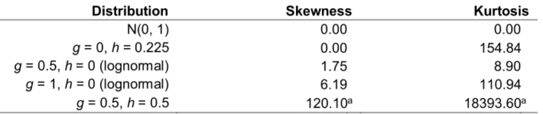
The four distributions used here were the standard normal (g = h = 0.0), a symmetric heavy-tailed distribution (h = 0.2, g = 0.0), an asymmetric distribution with relatively light tails (h = 0.0, g = 0.2), and an asymmetric distribution with heavy tails (g = h = 0.2). Table 1 shows the skewness (κ1) and kurtosis (κ2) for each

distribution. Additional properties of the g-and-h distribution are summarized by Hoaglin (1985).

The g-and-h distributions with h = 0.2 were chosen in an attempt to span the range of distributions that might be encountered in practice. The idea is that, if method G performs well for what some might regard as an unrealistic departure from normality, this provides some reassurance that it will perform reasonably when dealing with data from an actual study.

Three types of associations were considered. The first two deal with situations where

ij ij

Y X  .

The two choices for the slope were β = 0 and 1. The third type of association was

Y = X2 _{+ ε. These three situations are labeled S1, S2, and S3, respectively. The}

estimated Type I errors were very similar for S1 and S2, so for brevity only the results for S1 are reported.

The Xij values were generated from a standard normal distribution and ε was

generated from one of the four g-and-h distributions previously indicated.

Table 1. Some properties of the g-and-h distribution

g h κ1 κ2

0.0 0.0 0.00 3.00

0.0 0.2 0.00 21.46

0.2 0.0 0.61 3.68

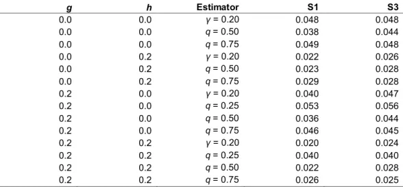
Table 2. Estimated Type I error probabilities when testing at the α = 0.05 level g h Estimator S1 S3 0.0 0.0 γ = 0.20 0.048 0.048 0.0 0.0 q = 0.50 0.038 0.044 0.0 0.0 q = 0.75 0.049 0.048 0.0 0.2 γ = 0.20 0.022 0.026 0.0 0.2 q = 0.50 0.023 0.028 0.0 0.2 q = 0.75 0.029 0.028 0.2 0.0 γ = 0.20 0.040 0.047 0.2 0.0 q = 0.25 0.053 0.056 0.2 0.0 q = 0.50 0.036 0.044 0.2 0.0 q = 0.75 0.046 0.045 0.2 0.2 γ = 0.20 0.020 0.024 0.2 0.2 q = 0.25 0.040 0.040 0.2 0.2 q = 0.50 0.022 0.028 0.2 0.2 q = 0.75 0.026 0.025

The simulation results are reported in Table 2. As can be seen, when testing at the 0.05 level, the actual level was estimated to be less than or equal to 0.056 among all of the situations considered. Although the seriousness of a Type I error depends on the situation, Bradley (1978) suggests that, as a general guide, when testing at the 0.05 level, the actual level should be between 0.025 and 0.075. Based on this criterion, the only concern is that, for a very heavy-tailed distribution, the estimated level drops below 0.025, the lowest estimate being 0.020. Increasing both sample sizes to 50 corrects this problem. For example, with g = h = 0.2 and γ = 0.2, the estimate for situation S1 increases from 0.020 to 0.034.

Notice that the lowest estimates in Table 2 occur for γ = 0.2 when g = h = 0.2. Simulations were run again with n1 = n2 = 100 as well as n1 = n2 = 200 as a partial

check on the impact of using larger sample sizes. The estimated Type I error probabilities for these two situations were 0.036 and 0.040, respectively.

As explained, there are at least three reasons to expect that the global test will have more power than method W. The extent to which this is true depends on the situation. To provide at least some perspective, consider the case where the covariate has a normal distribution and the error term has a g-and-h distribution. First consider g = h = 0 (normality) and suppose that the first group has β1 = β0 = 0

while, for the second group, Y = 0.5 + ε. With n1 = n2 = 50 and testing at the 0.05

level, the power of method G test was estimated to be 0.51. The probability of rejecting at one or more design points using method W was estimated to be 0.38. If instead Y = 0.5X + 0.5 + ε for the second group, the power estimates are now 0.75 and 0.66, respectively. If Y = 0.5X2 _{+ 0.5 + ε, the estimates are 0.89 and 0.78. For}

this last situation, if (g, h) = (0, 0.2), the estimates are 0.76 and 0.70. For (g, h) = (0.2, 0.2) the estimates are 0.75 and 0.70. So all indications are that G has more power, with the increase in power estimated to be as high as 0.12 among the situations considered here.

As already noted, a well-known argument for using a 20% trimmed mean, rather than the mean, is that under normality its efficiency compares very well to the mean. However, as we move toward a heavy-tailed distribution, the standard error of the mean can be substantially larger than the standard error of the 20% trimmed. That is, in terms of power, there is little separating the mean and 20% under normality, but for heavier tailed distributions, power might be substantially higher using a 20% trimmed mean. For the situation at hand, consider again

g = h = 0 and Y = 0.5 + ε, only now method W is applied using means rather than 20% trimmed means. Now power is estimated to 0.43, slightly better than using a 20% trimmed for which power was estimated to be 0.38. Using instead method G, power was estimated to be 0.56. So again, method G offers more power than method W and power is a bit higher compared to using a 20% trimmed mean, which was 0.51. For (g, h) = (0, 0.2), now the power of method W was estimated to 0.25 when using a mean compared to 0.48 when using a 20% trimmed mean. More relevant to the present paper is that, if method G is used with a mean, power is estimated to be 0.30, which is substantially smaller than the estimate of 0.51 when using a 20% trimmed mean.

Illustrations

There is the issue of whether method G can reject when method W does not when dealing with data from an actual study. There is also the issue of whether comparing quartiles makes a practical difference. This section reports results relevant to these issues using data from the Well Elderly 2 study.

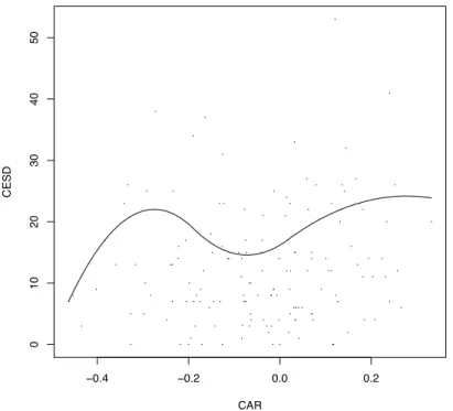
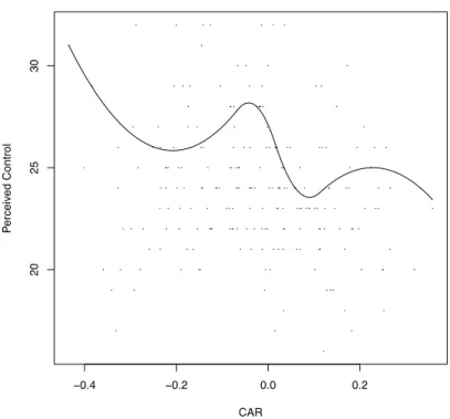
A general goal in the Well Elderly 2 study was to assess the efficacy of an intervention strategy aimed at improving the physical and emotional health of older adults. A portion of the study was aimed at understanding the impact of intervention on depressive symptoms as measured by the Center for Epidemiologic Studies Depressive Scale (CES-D). The CES-D (Radloff, 1977) is sensitive to change in depressive status over time and has been successfully used to assess ethnically diverse older people (Lewinsohn, Hoberman, & Rosenbaum, 1988; Foley, Reed, Mutran, & DeVellis, 2002). Higher scores indicate a higher level of depressive symptoms. Another dependent variable was the RAND 36-item Health Survey (SF-36), a measure of self-perceived physical health and mental well-being (Hays,

Sherbourne, & Mazel, 1993; McHorney, Ware, & Raozek., 1993). Higher scores reflect greater health and well-being.

Before intervention and six months following intervention, saliva samples were taken at four times over the course of a single day: on rising, 30 min after rising but before taking anything by mouth, before lunch, and before dinner. Then samples were assayed for cortisol. Extant studies (e.g., Clow et al., 2004; Chida & Steptoe, 2009) indicate that measures of stress are associated with the cortisol awakening response (CAR), which is defined as the change in cortisol concentration that occurs during the first hour after waking from sleep (i.e. CAR is taken to be the cortisol level upon awakening minus the level of cortisol after the participants were awake for about an hour). Here, the goal is to compare males and females after intervention based on CES-D and SF-36 measures using the CAR as a covariate.

To illustrate that in practice the global test can reject when method W does not, and that comparing lower or upper quantiles can make a practical difference, consider the goal of comparing males and females based on CES-D measures using CAR as a covariate. No differences are detected based on a 20% trimmed mean or median when using method W as well as the global test proposed here. This remains the case when comparing 0.25 quantiles using a bootstrap version of method W. But when using method G to compare the groups based on the 0.25 quantile, a significant difference is found. That is, there was no significant difference between males and females based on a measure of location intended to reflect the typical response. But the results indicate that there is a sense in which males tend to have even lower CES-D scores than females.

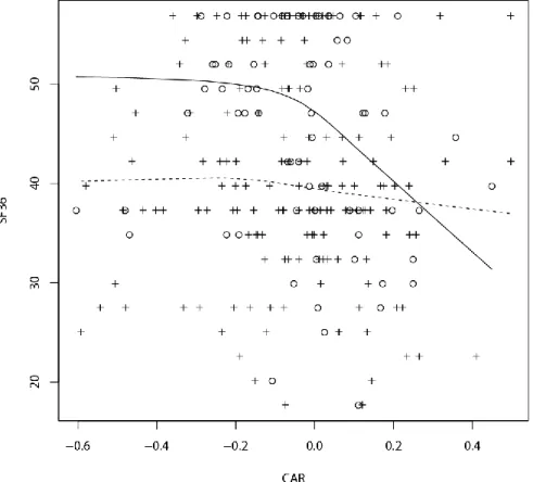
For the SF-36, testing (3) based on the median, a significant difference is found at the 0.05 level. There were 75 males and 171 females after eliminating missing values. Figure 1 shows a plot of the regression lines where the solid lines is the regression line for males. For the males, there were 6 outliers among the CAR values and, for the females, there were 8 outliers (based on a boxplot) which were eliminated from the analysis and are not shown in Figure 1. Eliminating outliers among the independent variable is allowed; it is eliminating outliers among the dependent variable that can cause technical problems. For the situation in Figure 1, a bootstrap version of method W indicates significant differences when CAR is negative (cortisol increases shortly after awakening). In practical terms, the results indicated that the typical male’s perceived health and well-being scores are higher among individuals whose cortisol levels increase after awakening. When cortisol decreases, no significant difference between males and females is found. Moreover, there appears to be little or no association between the CAR and SF-36 among